1. Introduction
In decision making, especially in complex contexts where multiple factors are involved, it is essential to have tools that allow the evaluation of various options in a structured and objective manner [
1]. Multi-criteria decision making (MCDM) methods emerge as an effective solution to analyze alternatives considering different criteria, often in conflict with each other. MCDM breaks down a complex problem into simpler parts, allowing the decision maker to structure a problem with multiple criteria in a visual way, by analyzing the mathematical models of each MCDM method [
2,
3,
4,
5,
6,
7,
8]. These methods are applied in areas as diverse as business management, engineering, economics, and urban planning, helping to select the best option among several possible ones. Unlike traditional optimization approaches, multi-criteria methods do not seek a single optimal solution, but rather allow balancing different priorities according to the needs of the decision maker.
One important stage in the product design process is the material selection, which is a fundamental aspect in the design and development of products for industrial applications [
3]. The right choice not only impacts the performance and efficiency of the product, but also its cost, durability, and sustainability [
5,
6,
7,
8]. In sectors such as manufacturing, construction, automotive, and aerospace, material selection determines key factors such as mechanical strength, corrosion resistance, thermal, and electrical conductivity, among others. Material selection is a vital part of the design phase. Choosing the right material to work with will ensure that your component is durable enough for its purpose. While there are tons of data that you can use during the selection process, there are also tests that you can do after production to ensure that your component is durable and robust. A poor choice of materials can lead to premature failures, increased maintenance costs and reduced product life, affecting the company’s competitiveness. Therefore, it is essential to have well-defined methodologies and criteria for the selection of materials, taking into account technical, economic, and environmental aspects.
One of the design tactics used to achieve product efficiency is MCDM for choosing materials [
2,
3,
4,
5,
6,
7,
8]. Since every product is different, it may require a range of features that cannot be met by a single material. Utilizing a range of materials in a design is a practical way to meet the functional requirements of a product. The employment of various materials in product design leads to a more practical, producible, economical, and aesthetically pleasing product, according to Ashby et al. [
9]. Comparative analysis of candidate materials is the foundation of MCDM approaches, according to the author of [
3]. They are techniques that help define the qualities of what is desired; therefore, in order to determine what the primary function will be, a list of candidates must be created before selecting one. According to the author of [
4], selecting an appropriate material for a product usually involves comparing and contrasting a variety of factors and material characteristics that are important when offering the material as a service.
Examples of using MCDM to resolve material selection can be found in the following studies. The Analytic Hierarchy Process (AHP) method is used for the phase change material selection for the thermal comfort in a vehicle where different phase change materials are tested to maintain a constant temperature inside a car cabin, without the need for air conditioning [
5]. MCDM methods such as COPRAS, VIKOR, ELECTRE I ARAS, MOORA, and ENTROPY have proven to be suitable methods to validate the selection of materials [
5,
6]. Bitarafan et al. [
6] looked at “Evaluating construction methods of cold-formed steel structures to reconstructed the areas damaged in natural crises, using the AHP and COPRAS-G methods”; Findik and Turan [
7] studied “Materials selection for lighter wagon design with a weighted property index method”; Zavadskas, et al. developed [
8] “Material selection for the tool holder working under hard milling conditions using different decision making methods”; and Çaliskan [
9] investigated the ”Selection of boron-based tribological hard coatings using multi-criteria decision making methods”.
However, it is crucial to confirm the MCDM findings. The design simulation helps producers validate and confirm a product’s intended use and manufacturing capabilities during the product development phase [
10,
11,
12]. Computer-aided engineering (CAE) is commonly referred to as “simulation” in a broad sense. Many design simulation techniques have become common parts of product development in various industries and are still becoming more relevant as a result of the effective, rapid, economical, and user-friendly design simulation software. Collections of mathematical formulas known as “simulation models” show how a system responds in a fascinating physical environment. The accessibility of the data determines the mathematical difficulty, which varies by application and design stage.
There are simulation examples for car parts in Anderson and Coughlan’s research [
13] on development of the flow of liquid over different surfaces and in Boutchel et al.’s study [
14] that uses wind tunnels to optimize real-world rain conditions. Gaylard and Duncan [
15] looked into how road sprays can soil a vehicle’s body side and rear glass, Roettger et al. [
16] looked into the consequences of contamination brought on by solid particle adhesion, and Wu and Cui [
17] investigated the behavior of a scale cargo ship in pools during swell. Some other examples were developed [
18,
19,
20,
21,
22,
23,
24,
25,
26,
27].
Disc brakes are designed to act through friction forces, this being the means by which the kinetic energy of the body to be decelerated is transformed into heat. Consequently, the brakes must be processed with materials that have good resistance to wear and thermal dissipation of the heat generated, so a good thermal conductivity is necessary. Furthermore, to inhibit the deformation of the element, a good Young’s modulus, elastic limit, and Poisson’s coefficient is preferred. A high value of hardness, compressive strength, and traction will prevent the material from fracturing. To reduce consumption, a low density of the material is preferred. To reduce the production costs of the vehicle and for this to be a factor for sales, it is necessary that the price of the brakes be as low as possible.
However, none of the above-mentioned research includes MCDM selection with simulation. The present study aims to evaluate brake disc material selection for brake discs in light SUV-type vehicles. Five different MCDM methods were used to select the best material alternatives and the ENTROPY method was used for weighting the criteria. In addition, a simulation is carried out to validate the results of the MCDM analysis and to show that the selected material can be used due to its strength and temperature conditions.
2. Materials and Methods
The physical, mechanical, and thermal properties of the candidate materials were taken from the Granta EduPack 2024 program and the MatWeb platform. Both platforms draw from validated industrial standards and are routinely updated, adding weight to the accuracy of the material property data. The candidate materials are presented in
Table 1.
With the data on the properties of the materials (Young’s modulus, compressive strength, yield strength, hardness, thermal conductivity, density, and specific heat) a comparison of all these properties is made with the proposed multi-criteria methods to find the best material for the desired application.
The friction coefficient and tribological properties of each material were not included as criteria for material selection because the focus was on the thermal, mechanical, and physical properties that directly impact the structural and thermal performance of brake discs. The MCDM methods used—like COPRAS, VIKOR, and ELECTRE—emphasize measurable and comparable data, such as yield strength, density, thermal conductivity, and hardness. While friction and tribological behavior are crucial for brake performance, they can be highly variable and context-dependent, often requiring experimental data rather than standard material property tables like those from CES EduPack 2024 or MatWeb 2024. Additionally, this study validated the material choice through thermal–structural simulation, prioritizing heat dissipation and structural integrity over surface interaction properties. Including tribological data would have added complexity to the MCDM models and might require real-world testing to gather reliable data.
2.1. Multi-Criteria Selection Methods and Weighting Method
COPRAS, VIKOR, ELECTRE I, ARAS, MOORA, and ENTROPY are the MCDM methods that have been used. As demonstrated in the bibliographic review, these are MCDM methods that have proven their worth for the best selection of a material among different alternatives. They are explained below.
2.1.1. ENTROPY Method
ENTROPY measures the uncertainty in information formulated using probability theory. According to Wang et al. [
21], the ENTROPY method could be calculated as follows:
Step 1: Building the decision matrix.
Step 2: Calculation of the normalized decision matrix
, using Equation (1).
Step 3: Calculation of ENTROPY
, using Equation (2)
where k =
is a constant that guarantees 0 ≤
≤ 1 and m is the number of alternatives.
Step 4: Calculation of the diversity of criteria D
j, by Equation (3).
Step 5: Calculation of the normalized weight of each criterion W
j, using Equation (4).
It is necessary to know the methodology of each MCDM method. It is important to emphasize which criteria are going to be considered as positive and negative during the development of the MCDM method; this consideration is shown in
Table 2, which will be used for all methods that require this consideration.
2.1.2. COPRAS Method
The COPRAS method selects the best decision alternatives by considering the ideal and worst-ideal solutions. It is used for its ability to directly account for both beneficial and non-beneficial criteria. It ranks alternatives by comparing their performance relative to an ideal and worst-ideal solution, making it effective for assessing trade-offs in material properties like strength versus cost. Goswami et al. [
22] develop the algorithm with the following steps:
Step 1: Calculation of the normalized decision matrix
.
Step 2: Calculate the weighted normalized decision matrix D
ij.
Step 3: Calculate S
i+ and S
i- of the normalized weighted values.
Step 4: Determine the relative importance of the
alternatives.
Step 5: Calculate
of each alternative, using the following Equation (10).
where
is the maximum value of relative importance.
2.1.3. VIKOR Method
The VIKOR compromise algorithm has the following steps used by Radovanović et al. in [
23]. It was selected for its focus on compromise solutions. This method identifies the alternative closest to the ideal solution, which is useful when no single material is perfect across all criteria, balancing high mechanical performance with reasonable costs and density. It has the following steps.
Step 1: Normalized decision matrix
Xij.
Step 2: Calculation of weighted normalized decision matrix f
ij.
Step 3: Determine the best
and the worst
-value of all the criterion.
Step 4: Distance to the positive ideal solution S
i and negative ideal solution
.
Step 5: Calculation of the values (Ii), for i = 1, …, I, is defined by Equation (17).
2.1.4. ELECTRE Method
The ELECTRE method has the ability to handle discrete quantitative and qualitative criteria and provides a complete ordering of the alternatives. It has been chosen due to its capacity to handle qualitative and quantitative data while considering pairwise comparisons. This method helps capture dominance relationships between materials, providing a clear picture of which options outperform others under conflicting criteria. Taherdoost et al. [
24] develop its calculus procedure as follows:
Step 1: Normalized decision matrix
rij calculus.
Step 2: Normalization of the decision matrix determination.
Step 3: Normalized weighted decision matrix (Vij) construction, according to Equation (20).
Step 4: C
ab concordance index matrix determination, it is obtained according to Equation (22).
Step 5: D
ab discordance index matrix calculation, using Equation (20).
Step 6: Calculation of the maximum threshold
for the concordance index and the maximum threshold
for the discordance index, using Equations (24) and (25), respectively.
Step 7: Development of the dominant concordance matrix
. It is calculated by the following condition:
Step 8: Calculation of the dominant discordant matrix
using the following condition:
Step 9: Calculation of the aggregate dominance matrix (concordance–discordance)
, using Equation (28).
Step 10: Calculation of the upper and lower net value Ca and Da.
2.1.5. ARAS Method
The ARAS method determines the complex relative efficiency of a feasible alternative. It has been applied because of its straightforward approach to calculating the relative efficiency of each alternative. It effectively integrates both material attributes and their weights, making it ideal for highlighting materials with the most balanced performance. The steps of this method are as follows, as found in Zavadskas and Turskis [
25]:
Step 1: Formation of the decision matrix X
ij using Equation (31).
Step 2: Calculation of the normalized decision matrix
-
where
=
For non-beneficial criteria it is calculated using
=
;
=
.
Step 3: Determination of the weighted normalized decision matrix i
(33).
Step 4: Calculation of the optimization function S
i. Where S
i value of the optimization function of the i alternative using Equation (35).
Step 5: Calculation of the degree of utility K
i. Where S
i and S
o are the values of the optimization function (30).
2.1.6. MOORA Method
The MOORA method starts from reference points, which will be the highest evaluation of the vector of alternative radii with respect to each criterion, whether maximum or minimum [
12]. It has been used for its simplicity and reliability in solving complex decision-making problems. By comparing alternatives against reference points, it highlights materials that stand out in both beneficial (strength, thermal conductivity) and non-beneficial (density, cost) criteria. To the determinate the solution, the following steps should be developed:
Step 1: Determination of the decision matrix X
ij (37).
Step 2: Calculation of the radius matrix of the form
=
(38).
Step 3: Weight vector calculus of each the criteria.
Step 4: Normalized weighted matrix.
Step 5: Calculation of the aggregation function to evaluate each alternative S(x
i) using Equation (39).
The inclusion of these five methods allows for a comprehensive comparison from multiple analytical perspectives, reducing bias and enhancing the reliability of the final material ranking. The ENTROPY method was further employed to objectively assign weights to each criterion based on the degree of variability, ensuring that the most influential properties—such as yield strength and thermal conductivity—carried appropriate importance in the decision-making process.
2.2. MCDM Results
The multi-criteria results and the simulation results are based on reference [
18].
2.2.1. ENTROPY Method
The values of the physical, mechanical, and thermal properties of the candidate materials are taken from
Table 1 to prepare the standard decision matrix that will be used to calculate the MCDM, which is expressed in
Table 3.
The normalized decision matrix values Pij, are shown on
Table 4.
The normalized matrix of the Ei is shown in
Table 5.
The calculation of the diversity of the criterion (Dj) is shown in
Table 6.
Finally, the weight of the criteria Wj is calculated in
Table 7.
2.2.2. COPRAS Method
The weighted normalized decision matrix (Dij) is determined, which is obtained by multiplying the weight of each criterion obtained by the ENTROPY method, with the values of the normalized matrix. The values are presented in
Table 8.
The weighted normalized decision matrix (Dij) is determined by multiplying the weight of each criterion obtained by the ENTROPY method with the values of the normalized matrix and is shown in
Table 9.
Normalized weight values are determined for beneficial (
and non-beneficial (
) criteria. The values of these parameters are shown in
Table 10.
The relative priorities of the alternatives (
) are calculated and they are shown in
Table 11.
The performance index (
) of each alternative is calculated and shown in
Table 12. Taking into account that the highest value of this parameter indicates the ranking of the alternatives.
2.2.3. VIKOR Method
The development of the normalized initial decision matrix (fij) is shown in
Table 13.
The best (
) and worst (
) values of all the criterion functions for each alternative were determined. If the ith function represents a benefit, then
= max
j f
ij and
= min
j f
ij, while the ith function represents a cost. These values are represented in
Table 14.
The representation at the ideal value is shown in
Table 15. ASTM A48 represents the best option.
2.2.4. ELECTRE Method
The normalization of the decision matrix is represented in
Table 16.
For the construction of the normalized weighted decision matrix (V
ij), the normalized decision matrix (r
ij) is multiplied with its respective weight, and is shown in
Table 17.
The concordance index (C
ab) is calculated between the alternatives (r
ij) by adding the weights associated with the criteria in which alternative i is better than alternative j or vice versa (
Table 18).
The discordance index (D
ab), between alternatives
and
is calculated as the largest difference between the criteria for which alternatives i is dominated by
, then divided by the largest difference in absolute value between the results obtained by alternative
and
. The values are shown in
Table 19.
Calculation of the aggregate dominance matrix (concordance–discordance). The elements of this matrix are calculated by multiplying the homologous values of the concordant dominance matrix and the discordant dominant matrix. These values are shown in
Table 20.
Finally, the alternative ranking is presented in
Table 21.
2.2.5. ARAS Method
The normalized weight decision matrix
, is represented in
Table 22.
The optimization function
Si and the degree of utility K
i are calculated. This degree is determined by comparing the variant being analyzed with the best So (
Table 23).
2.2.6. MOORA Method
The radius matrix of the form
=
is calculated to normalize the initial decision matrix (
Table 24).
The normalized matrix is calculated by weights and it is presented in
Table 25. It is weighted by multiplying the normalized decision matrix by the weights of each criterion.
The aggregation function is determined to evaluate each alternative S(xi), which is shown in
Table 26.
2.3. Simulation
A thermal phenomenon analysis can be performed by determining the heat produced by the effect of friction as it occurs in the real braking phenomenon. It is necessary to know which ANSYS 2024 modules allow this type of transient thermal analysis to be performed. To obtain the geometry of the brake disc, the 3D Scanner was used as explained above. To draw the geometry of the brake disc, the Siemens NX software 2024 was used. ANSYS allows direct linking with NX files, without losing any detail generated in it. On the other hand, the brake pad was designed following the manufacturer model Bosch D1185 (Gerlingen, Germany); however, the material was considered the same as the disc.
Thermal analysis of the brake disc requires an accurate determination of the total frictional heat generated and how this energy is distributed between the disc and the pads. The purpose of thermomechanical analysis is to predict temperatures and the corresponding thermal stresses and deformations in the brake disc.
For this analysis, the TARGE 170 and CONTA 174 type meshes are used. The TARGE 170 type mesh is used to represent several three-dimensional “target” surfaces for the associated contact elements. The contact elements themselves are superimposed on the solid, frame or line elements. The element is applicable to structural and coupled field three-dimensional contact analyses. It can be used for both pairwise contact and general contact.
Figure 1 shows the meshed brake disc and pad, emphasizing that the mesh has a precision of 0.994, taking into account that the ideal is 1 as shown in the figure.
The simulation was made with the Transient Structural module, where the boundary conditions declared are as follows:
where b =
=
= 0.06745 m
ΔTmax represents the maximum temperature variation that a brake disc undergoes to stop a vehicle traveling at 90 km/h. An ambient temperature of 16 °C was assumed, so the final temperature of the brake disc will be Tf = 187.42 °C + 16 °C → Tf = 203.42 °C.
The final temperature of the disc is transferred to the pads in a conductive way while a convection is declared to analyze the cooling on the fins.
The material is declared as a basic material in ANSYS with an isotropic behavior with a constant density, neglecting a volume change by temperature. The selected material, which is ASTM A536, is placed on all assembly parts of the brake disc and pads.
The force applied to the drag face of the brake disc is 2500 N. This force must be applied at the interface on the faces of the disc and the brake pad that are in contact, as shown in
Figure 2b. These values are taken into account after previous calculations.
3. Results
The results of the brake disc material selection based include the multi-criteria results and the simulation results.
Simulation
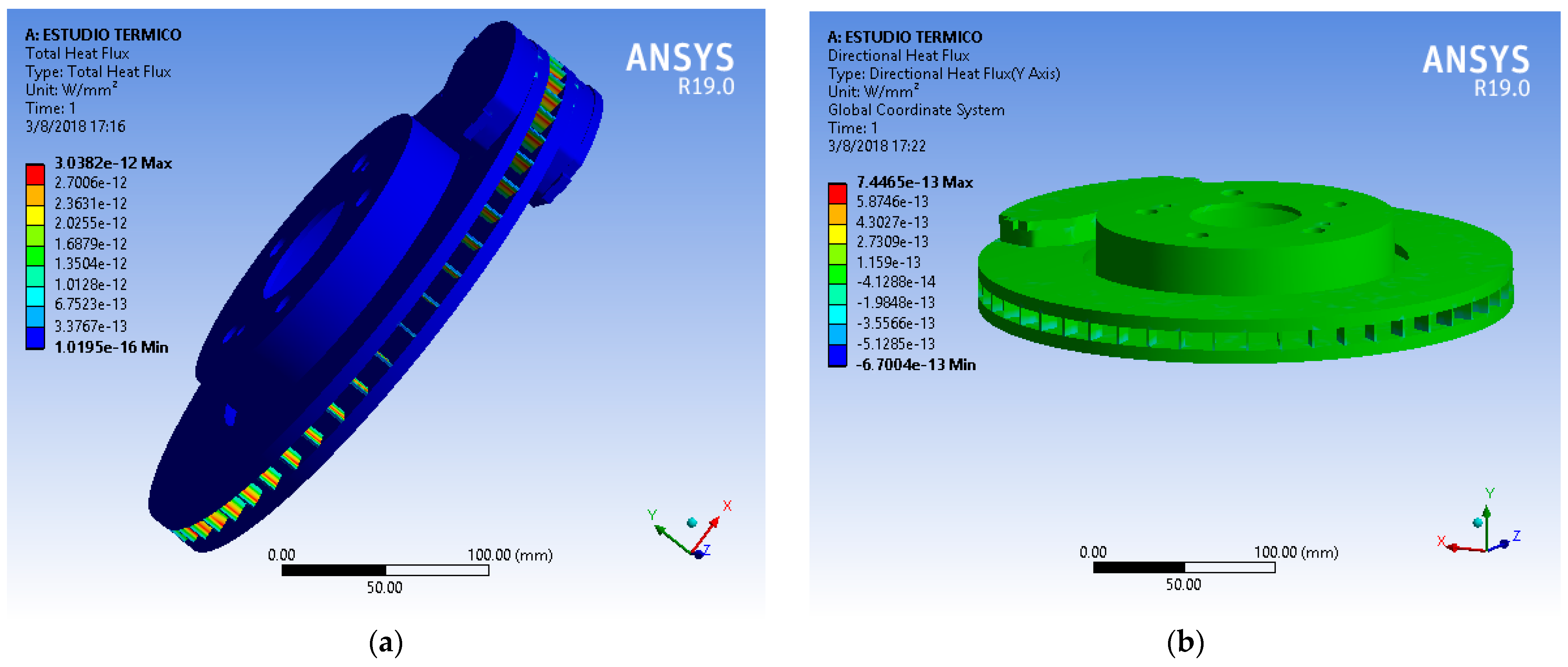
Once the boundary conditions are set, ANSYS allows us to visualize the heat flow produced in the system; the directional flow, that is, on the Y axis, since we are interested in knowing how the heat flows from one end to the other end and the interaction of the fins. With the thermal–structural study, we intend to verify the resistance of the selected material to the two types of load, both the static load due to the effect of the pressure and force exerted by the caliper, as well as the thermal load that is defined by the final temperature of the disc, which is 203.42 °C, and an initial temperature or ambient temperature of 16 °C. So, in the thermal study, we have two types of results such as the total heat flow that can be seen in the heat variation, that is, the convection and conduction process that exists in the disc that, logically, will occur in the fins, as shown in
Figure 3a. A directional flow process can also be observed, i.e., only the flow component on the Y axis as shown in
Figure 3b.
In the structural study, the forces applied to the caliper are combined with the final temperature of the disc to determine the total deformation of the brake disc under the aforementioned working conditions. This deformation is 0.0650 mm, which can be said to be acceptable.
Figure 4a shows the deformation of the brake disc. The equivalent stress is 122.86 MPa, which, when contrasted with the yield stress allowed by this ASTM A536 material, is 5.29, which is the safety factor shown in
Figure 4b. In this sense, the results of the simulations show that the selection of the material is adequate and also the best.
4. Discussion
The material ranking results obtained from the MCDM methods (COPRAS, VIKOR, ELECTRE I, ARAS, MOORA) reflect a comprehensive evaluation of the physical, mechanical, and thermal properties of the candidate materials. The primary factors considered in the selection process were yield strength, density, hardness, compressive strength, thermal conductivity, and price. Each method provided a systematic approach to balance these criteria, ensuring that the best material was chosen based on a well-rounded perspective [
3,
4,
5].
The consistent ranking of ASTM A536 as the top choice in the COPRAS, ELECTRE I, and ARAS methods can be attributed to its combination of favorable mechanical properties. Its high yield strength (339 MPa), good compressive strength (351 MPa), and moderate density (7150 kg/m3) present an optimal balance between durability and weight—a critical factor for light SUV brake discs. The simulation results further confirmed its suitability, revealing that ASTM A536 maintained structural integrity under thermal and mechanical loads, with a total deformation of only 0.0650 mm and an equivalent stress of 122.86 MPa, resulting in a safety factor of 5.29. ASTM A48 was ranked second by the COPRAS and ARAS methods, due to its high hardness (252 HV) and good thermal conductivity (46 W/m °C). These attributes contribute to the material’s ability to withstand wear and dissipate heat efficiently during braking. However, its lower yield strength (149 MPa) compared to ASTM A536 likely affected its overall score, particularly in methods that heavily weighted mechanical resilience. Al10SiC emerged as a strong alternative, ranking second in VIKOR and MOORA. This material’s low density (2770 kg/m³) and excellent thermal conductivity (148 W/m °C) make it highly desirable for heat dissipation and weight reduction. The material’s tensile strength (372 MPa) and compressive strength (358 MPa) also position it as a viable option for enhancing brake disc performance. The relatively higher price (8.29 USD/kg) may have negatively impacted its ranking, particularly in methods considering cost as a crucial factor. Interestingly, AISI 304L, despite its superior yield strength (310 MPa) and excellent corrosion resistance, ranked lower across all methods. Its high density (7980 kg/m3) added unnecessary weight, and its moderate thermal conductivity (16 W/m °C) limited its effectiveness in dissipating heat. These shortcomings highlight the trade-offs between mechanical strength and thermal performance, emphasizing the importance of balanced criteria in material selection.
Automotive manufacturers prioritize cost-effective solutions to maintain competitive pricing. An affordable brake disc directly affects the overall vehicle price, which is crucial in price-sensitive markets like light SUVs. Lower-cost materials, like ASTM A536 and ASTM A48 (both priced at USD 0.67/kg), reduce production expenses, making the final product more affordable and potentially boosting profit margins. More expensive materials, such as Ti 6Al 4V (USD 27.5/kg), may only be viable for high-performance or luxury applications due to their impact on production costs.
The simulation results play a key role in validating the rankings obtained through the MCDM analysis by providing insight into how different material and design choices affect thermal and mechanical performance. The thermal–structural study helps assess the selected material’s resistance to both static and thermal loads. The static load stems from the pressure and force exerted by the caliper, while the thermal load is defined by the temperature variation—from an ambient temperature of 16 °C to a final disc temperature of 203.42 °C. The thermal analysis produces two key results: the total heat flow, which reveals the heat variation due to convection and conduction within the disc and fins, which illustrates the primary heat transfer path. These findings directly support the MCDM ranking by confirming whether the top-ranked material and design choices meet the expected thermal performance criteria.
The structural analysis integrates the forces applied to the caliper with the final disc temperature to evaluate the total deformation of the brake disc under operational conditions. The observed deformation is within acceptable limits, as shown. Additionally, the equivalent stress reaches 122.86 MPa, which, compared to the yield stress of ASTM A536, results in a safety factor of 5.29. These results validate the material selection, aligning with the MCDM rankings that identified ASTM A536 as an optimal choice based on mechanical performance and thermal resistance. Thus, the simulation outcomes reinforce the MCDM-based selection process, confirming that this material ensures structural integrity and reliability in braking applications.
The absence of tribological properties (such as friction coefficient and wear rate) in the decision matrix may have influenced the rankings. While mechanical and thermal characteristics directly impact the structural integrity and heat management of the brake disc, tribological behavior governs friction performance and wear resistance—both crucial for braking efficiency. Future studies could integrate these properties, either through experimental testing or advanced simulation models, to capture a more holistic view of material performance.
Ultimately, the alignment of the MCDM results with the simulation findings reinforces the robustness of the material selection process. ASTM A536′s dominance across multiple methods and its strong validation in thermal–structural simulations solidify its position as the optimal choice for light SUV brake discs. Nevertheless, the strong performance of Al10SiC and ASTM A48 suggests that these materials warrant further investigation, particularly for applications prioritizing lightweight design and thermal efficiency.
5. Conclusions
The MCDM methods used in this research allowed the selection of a material for the manufacture of a brake disc, incorporating quantitative and qualitative criteria. For the three methods, the best material is ASTM A536, with better thermal and mechanical properties. In a second option according to the three methods, Al10Si C and ASTM A48 are chosen.
In the structural–thermal simulation, it is observed that the heat flow generated in the disc is efficient, since the heat transfer is generated in the fins. The total deformation of the brake disc when applying a force from the caliper and being subjected to a final operating temperature is 0.0650 mm. The presence of very high stresses is due to the thermoelastic distortions that occur due to friction, it can be mentioned that the equivalent stress is 122.86 MPa which, when contrasted with the yield stress allowed by this ASTM A536 material, gives a safety factor of 5.29, since it is a brittle material.
Future studies could integrate friction coefficient, wear rate, and tribological behavior into the MCDM framework. This would provide a more comprehensive evaluation of materials, especially for components like brake discs where surface interactions directly affect performance. Research could explore the environmental footprint of brake materials, considering particulate emissions, life-cycle analysis (LCA), and sustainability metrics. Adding these factors to MCDM could align material selection with green engineering principles.


