Article

A Fast Simulation Method for Predicting the Production Behavior of Artificial Fractures Based on Diffusive Time of Flight

1
Shale Gas Research Institute, PetroChina Southwest Oil & Gas Field Company, Chengdu 610051, China
2
School of Energy Resources, China University of Geosciences (Beijing), Beijing 100083, China
*
Authors to whom correspondence should be addressed.
Processes 2025, 13(4), 984; https://doi.org/10.3390/pr13040984
Submission received: 5 March 2025 / Revised: 19 March 2025 / Accepted: 24 March 2025 / Published: 26 March 2025

Abstract

:
Multi-stage hydraulic fracturing is a widely used technology in the development of shale oil and gas reservoirs that creates artificial fractures and forms fracture networks that enhance fluid flow within reservoirs. A well-designed fracture network can significantly enhance the production performance of oil and gas wells, thereby improving the recovery of shale oil and gas reservoirs. To achieve this, understanding the gas production performance of individual artificial fractures is crucial, as it provides valuable insights for refining subsequent fracturing designs, ultimately leading to an optimized fracture network design. At present, numerical simulations are commonly used to study the production performance of individual artificial fractures by modeling the production process of the entire shale oil and gas reservoir. However, due to the heterogeneity of reservoirs and the presence of numerous natural fractures, traditional numerical simulations require high-resolution grids to model the production process, making them computationally expensive and time-consuming. To address this issue, in this work, based on the concept of diffusive time of flight (DTOF), the authors propose a fast simulation method to efficiently simulate the production behavior of individual artificial fractures throughout the shale oil and gas reservoir production process. The DTOF can be obtained by solving the Eikonal equation using the fast marching method (FMM), which is then used to calculate the drainage volume of individual artificial fractures. Subsequently, a geometric approximation of the drainage volume is used to efficiently compute the production rates of individual artificial fractures. Unlike traditional numerical simulations, this method uses a single non-iterative calculation to determine the drainage volume of individual artificial fractures, followed by a geometric approximation to compute the production rates. This eliminates the need for high-resolution grids, significantly reducing computational cost and time, which allows the proposed method to provide faster simulations compared to traditional numerical methods while maintaining sufficient accuracy.

1. Introduction

Shale gas resources have attracted growing attention in recent years due to the depletion of conventional oil and gas reserves [1,2]. With low carbon dioxide emissions and zero sulfur dioxide content, shale gas represents an environmentally preferable energy source, particularly when compared to conventional fuels such as oil and coal [3,4,5]. Due to the low porosity and permeability of shale gas reservoirs, multi-stage hydraulic fracturing is commonly used to enhance their development by creating artificial fractures and forming complex fracture networks. These networks provide high-permeability pathways, significantly facilitating fluid flow within the reservoirs [6,7,8]. The development of shale gas reservoirs is highly influenced by the design of multi-stage hydraulic fracturing, as it determines the capacity of fracture networks to enhance fluid flow and increase production. To optimize multi-stage hydraulic fracturing design, it is crucial to simulate the production behavior of individual artificial fractures under varying fracture parameters [9,10]. At present, this is usually achieved by simulating the production process of the entire reservoir. However, shale gas reservoirs are highly heterogeneous and contain complex fracture networks, requiring high-resolution grids in each simulation to accurately represent the reservoir properties and fracture interactions [11]. This significantly increases the computational cost. Moreover, determining optimal fracture parameters requires running numerous simulations, which further increases the computational costs and time. Therefore, improving the efficiency of simulating the production behavior of individual artificial fractures is essential for optimizing multi-stage hydraulic fracturing design in shale gas reservoirs.
To address the challenge of high computational cost, recent advancements have focused on improving the efficiency of numerical simulations. One such approach is the concept of diffusive time of flight (DTOF), which represents the travel time of the peak pressure disturbance from an impulse source or sink to a certain point in the reservoir [12,13]. The DTOF can be rapidly obtained by solving the Eikonal equation using the fast marching method (FMM) [13,14] and can then be used to improve the computational efficiency of numerical simulations. Zhang [15] proposed a fast simulation method that involves transforming fluid-transport coordinates from the physical 3D space to the 1D DTOF space. The results show that by transforming high-dimensional equations into low-dimensional equations, the proposed method can significantly reduce computational time while maintaining accuracy. Teng [16] proposed a fast simulation method by using DTOF to reduce the model size. Their results indicate that focusing exclusively on simulating the regions affected by production can significantly reduce the number of grids used in simulation, thereby decreasing computational time. Lu [17] proposed a new approach for determining the control volumes of production wells using DTOF. The results indicate that fracture length, well distribution, and the number of wells substantially affect control volumes, whereas fracture conductivity has a negligible impact. Chen [18] developed a rapid simulation method using a multidomain, multiresolution discretization scheme based on the DTOF. The results show that by partitioning the reservoir into local and shared domains using DTOF contours, this method can provide fast and sufficiently accurate simulation results regardless of the production regime of the wells. More applications of DTOF can be found in Zhang [19], Fujita [20], and Iino [21]. However, DTOF has not yet been used to evaluate the production performance of individual artificial fractures in hydraulically fractured reservoirs.
According to the aforementioned arguments, one can find that improving the efficiency of simulating fracture production behavior is crucial for optimizing multi-stage hydraulic fracturing design, while the concept of DTOF can be used to enhance the simulation efficiency. Therefore, in this work, based on the concept of DTOF, the authors propose a fast simulation method to efficiently simulate the production behavior of individual artificial fractures. Furthermore, the proposed method is used to investigate the effects of various geological and fracture parameters on the production behavior of individual artificial fractures, as well as on well productivity.

2. Methodology

In this section, the authors first introduce the Eikonal equation and the fast marching method (FMM) for calculating the diffusive time of flight (DTOF), followed by an introduction to the calculation of the drainage volume of individual artificial fractures using the obtained DTOF. Then, the production calculation based on a geometric approximation of the drainage volume is presented in detail.

2.1. Drainage Volume Calculation Using DTOF

The conservation of mass for isothermal gas flow within the gas reservoirs is described by the well-known continuity equation, which is given by Al-Hussainy [22]:
ρ g v = ρ g ϕ t
where ρg is gas density, v is gas flow rate, ϕ is porosity, and t is time. The gas flow rate can be calculated by Darcy’s law [23]:
v = k μ g p
where k is permeability, μg is gas viscosity, p is pressure. The gas properties such as density, compressibility, and viscosity are highly pressure-dependent, which makes the gas flow equations nonlinear. This pressure-dependent nonlinearity complicates the solution process of Equation (1). The normalized pseudo-pressure and normalized pseudo-time are often used to linearize the gas flow equations, facilitating their solution. The normalized pseudo-pressure is defined as [22]
p p n = μ g Z p i 0 p p μ g Z d p
where Z is compressibility factor, p is pressure, and i is the initial state. Similarly, the normalized pseudo-time is defined as [24]
t p n = μ g c t i 0 t 1 μ g c t d t
where ct is total compressibility. Incorporating Equations (3) and (4) with Equation (1) yields
p p n t p n = k ϕ μ g c t i 2 p p n
The form of Equation (5) (i.e., gas diffusion equation) is consistent with the oil diffusion equation. Similar to the derivation of the Eikonal equation for describing the propagation of pressure disturbances within an oil reservoir [25], the equation for describing the propagation of the pseudo-pressure front within a gas reservoir can be derived from the gas diffusion equation (Equation (5)), which can be expressed as
k ϕ μ g c t i τ = 1
where τ is the propagation time of the pseudo-pressure front (i.e., diffusive time of flight). It is worth noting that the gas viscosity and total compressibility used in Equation (8) are taken at the initial reservoir conditions.
The Eikonal equation (i.e., Equation (6)) can be efficiently solved by the fast marching method (FMM). The detailed solution procedure can be found in Teng [16] and Zhang [19]. By solving the Eikonal equation using the FMM, the distribution of τ values in the entire reservoir can be obtained. However, the τ cannot be directly used to determine the drainage volume. Since τ is a parameter used in the simulation to represent pseudo-pressure disturbance, it is not directly related to pseudo-time. Therefore, the τ values distribution needs to be converted into the pseudo-front-time distribution [16,26]:
t f , p n = τ 2 β
where tf,pn is the pseudo-front time, which refers to the shortest pseudo-time that the pseudo-pressure disturbance reaches in a certain position, and β is the time conversion factor. For homogeneous reservoirs, the factor β depends on the flow geometry: β = 2, 4, and 6 for linear, radial, and spherical flows, respectively [25]. For heterogeneous reservoirs, β should be determined based on specific reservoir conditions. In this work, despite considering reservoir heterogeneity, the conversion factor for radial flow (β = 4) is used for the two-dimensional calculations. Subsequently, the drainage volumes at a given pseudo-time can be calculated by contouring the corresponding pseudo-front time and by summing up the pore volumes inside the contour.

2.2. Production Rate Calculation with Geometric Approximation

For radial flow in shale gas reservoirs, the gas mass flow rate under normalized pseudo-time can be described using Darcy’s law [23]:
q m r , t p n = ρ g k A r μ g p r , t p n r
where ρg is gas density, qm is gas mass flow rate, r is the distance from the wellbore, tpn is normalized pseudo-time, k is permeability, A is flow area, μg is gas viscosity, and p is pressure.
To derive the gas production rate, the Darcy flow equation (i.e., Equation (8)) is integrated over the drainage volume. The geometric approximation of the drainage volume is obtained using the fast marching method (FMM), and the pseudo-steady-state flow assumption is applied to facilitate the calculation, which is widely adopted in shale gas production prediction, as demonstrated in previous studies [27,28]. Consequently, the gas production rate can be expressed as
q r t p n = T s c T p s c p μ g Z i p ¯ p n p p n , w f 0 V p t p n 1 k ϕ A 2 1 V V p ( t p n ) d V
where psc and Tsc are pressure and temperature under standard conditions, respectively, T is reservoir temperature, Z is compressibility factor, p n ¯ is the average pseudo-pressure of the drainage volume, Ppn,wf is pseudo-pressure of wellbore, Vp is drainage volume, V is specific volume within the drainage volume, k is average permeability of the drainage volume, ϕ is average porosity of the drainage volume, A is the flow area. The detailed derivation of this equation is provided in Appendix A.

2.3. Framework of the Proposed Method
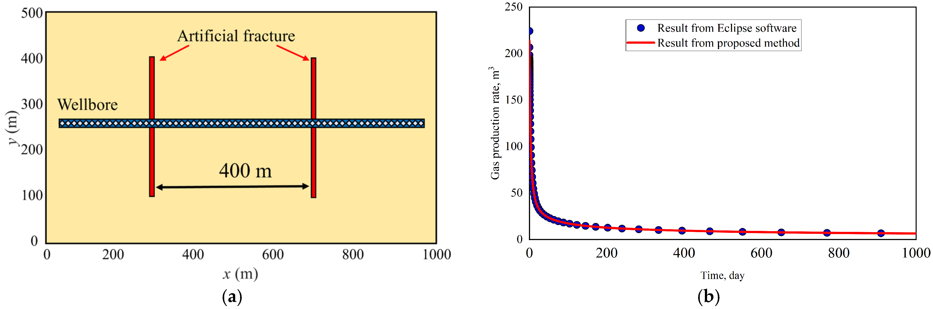
The key aspect of our proposed method is to use the pseudo-front time to divide the hydraulically fractured reservoir model into independent subdomains associated with each artificial fracture. The gas production rate for each artificial fracture is then calculated using the volume of its corresponding subdomain. Figure 1 schematically shows the simulation framework of the proposed method. As one can see in this figure, the simulation steps are as follows:
Firstly, calculate the pseudo-front time distribution of pressure disturbance propagation in the reservoir with each artificial fracture respectively by using FMM to solve Equation (6) (as described in Section 2.1) (see Figure 1a).
Secondly, divide the reservoir into independent subdomains by comparing the pseudo-front times at each location with each artificial fracture. If the pseudo-front time corresponding to artificial fracture 1 is the smallest, it can be inferred that the reservoir volume contributes to the production of artificial fracture 1 earlier than that of other artificial fractures. Therefore, this volume can be considered as part of the control volume for artificial fracture 1 (see Figure 1b).
Finally, calculate the gas production rate for each artificial fracture using Equation (9) based on the volume of the independent subdomains (as described in Section 2.2) (see Figure 1c).

3. Validation

To examine the validity and reliability of the proposed method for gas production calculation, the simulated results are compared to the results of the commercial software Eclipse 2006.1. The validation is conducted on a 2D shale gas reservoir model with two artificial fractures, which is shown in Figure 2a. As shown in Figure 2a, the artificial fracture spacing is 400 m. The reservoir dimensions are 1000 × 500 × 20 m, with a porosity of 0.2 and a permeability of 0.01 mD. The artificial fracture (red lines) length is 300 m, with a width of 0.01 m, a porosity of 0.5, and a permeability of 1 × 10⁶ mD. The reservoir temperature is 125 °C, the initial reservoir pressure is 25 Mpa, and the wellbore pressure is maintained at a constant value of 5 MPa. The extraction time t is 1000 days. Figure 2b compares the gas production rates obtained from Eclipse and the proposed method. It can be seen from this figure that the gas production rate from the proposed method shows a good agreement with the Eclipse software, indicating that the proposed DTIV-EDFM method can effectively calculate the gas production of shale gas reservoirs.

4. Result and Discussion

In this section, heterogeneous shale gas reservoir models with different conditions are established to investigate the effects of various geological and fracture parameters on the production behavior of individual artificial fractures, as well as on the well productivity. It is important to clarify that our study employs a two-dimensional (2D) model. While we describe the reservoir dimensions as 2000 × 1200 × 10 m to provide realistic lateral extent and thickness, the vertical dimension (10 m) is not explicitly incorporated into the simulation framework, as our method is specifically designed for 2D analysis. This choice is made to reduce computational complexity while capturing the lateral distribution and production behavior of fractures, which are typically the primary focus in shale gas reservoir optimization. The benchmark shale gas reservoir model is shown in Figure 3a. The artificial fracture (red lines) length is 300 m, with a width of 0.01 m and a compressibility of 1.2 × 10⁻³ MPa−1. The randomly generated natural fractures (black lines) within the reservoir range in length from 10 to 100 m, with a width of 1 × 10⁻2 m and a compressibility of 1.2 × 10⁻³ MPa−1. Figure 3b shows the porosity distribution of the shale gas reservoir. As shown in this figure, the matrix porosity is non-uniformly distributed, with higher values on the left and gradually decreasing values towards the right. The average porosity of the shale gas reservoir is 0.15. Figure 4a,b illustrate the permeability distribution along the x and y directions, respectively. Similar to the porosity distribution, the matrix permeability decreases from left to right in both the x and y directions. The average permeability of the shale gas reservoir in both the x direction and y direction is 0.01 mD. The values of other parameters applied in the benchmark shale gas reservoir models are shown in Table 1.

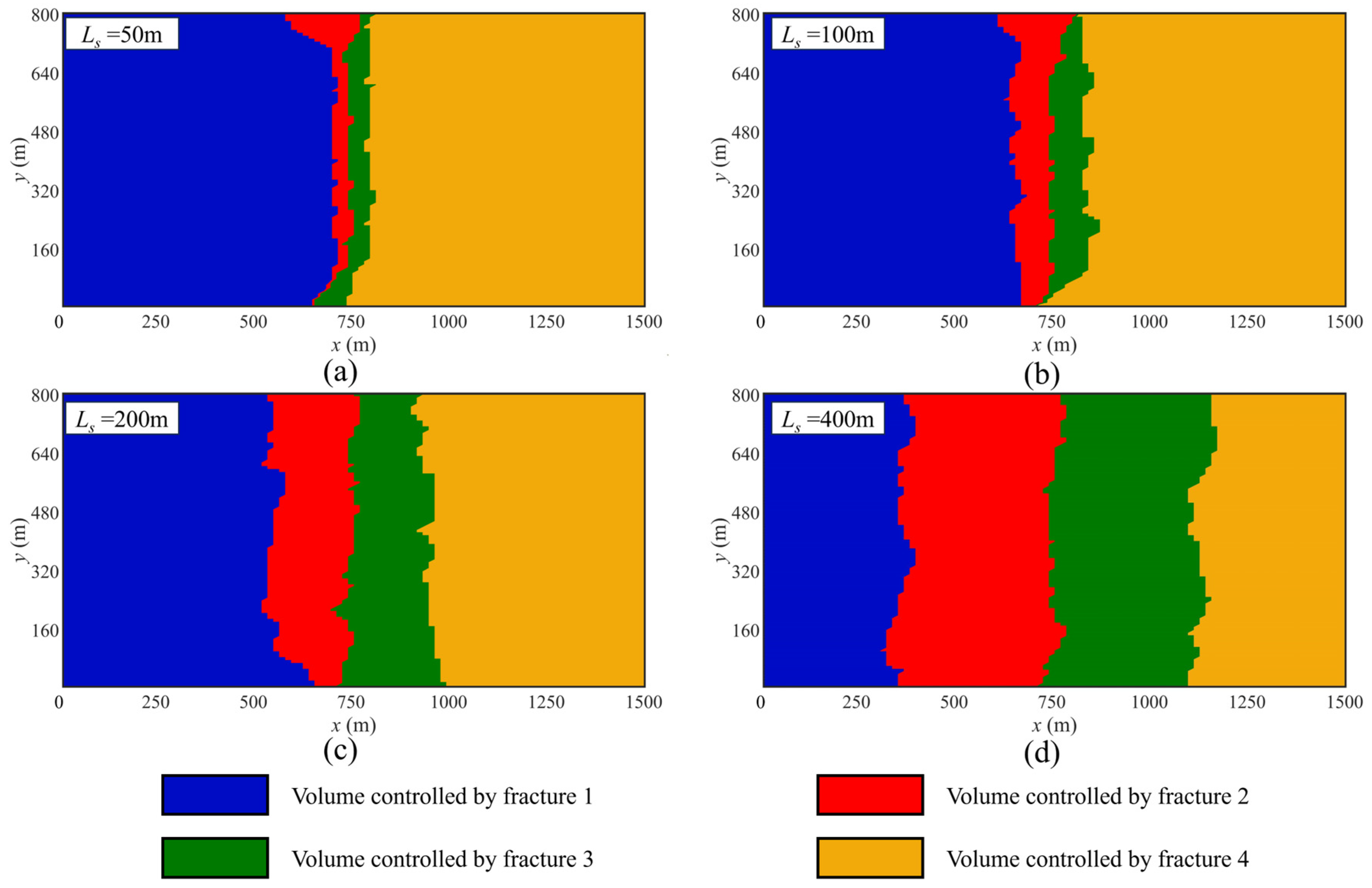
4.1. Artificial Fracture Spacing

The artificial fracture spacing is varied from 50 m to 200 m to examine its impact on both the control volumes and production performance of each artificial fracture, as well as on the well productivity. Figure 5 illustrates the distribution of the controlled volume of each artificial fracture with different artificial fracture spacing. As observed in the figure, when the artificial fracture spacing is small, the controlled volume of fracture 2 (red region) and fracture 3 (green region) only corresponds to a small portion of the surrounding volume. This occurs because the close spacing between fractures restricts their influence on the surrounding reservoir. As the artificial fracture spacing increases, the controlled volumes of fractures 2 and 3 gradually expand, reflecting their increased influence on a larger portion of the surrounding reservoir. This trend is further evidenced in Figure 6a, where the variation in controlled volume with artificial fracture spacing is shown quantitatively. Figure 6b compares the cumulative gas production of each artificial fracture and the well with varying artificial fracture spacing (calculated by Equation (9)). As the artificial fracture spacing increases, the cumulative production of the well increases. Specifically, as the fracture spacing increases from 50 m to 400 m, the cumulative gas production from the well rises significantly from approximately 8.05 × 10³ m3 to 1.71 × 10⁴ m3, representing an increase of about 112%. This is primarily because, with larger fracture spacing, the cumulative production from fracture 1 (blue dotted line) and fracture 4 (yellow dotted line) shows little change, while the cumulative production from fracture 2 (red dotted line) and fracture 3 (green dotted line) increases significantly. This is because the controlled volumes of fractures 2 and 3 expand as the artificial fracture spacing increases, leading to a greater contribution to the well’s cumulative production. This trend is consistent with the results shown in Figure 4, where the total controlled volumes of fractures 2 and 3 increase with larger fracture spacing.

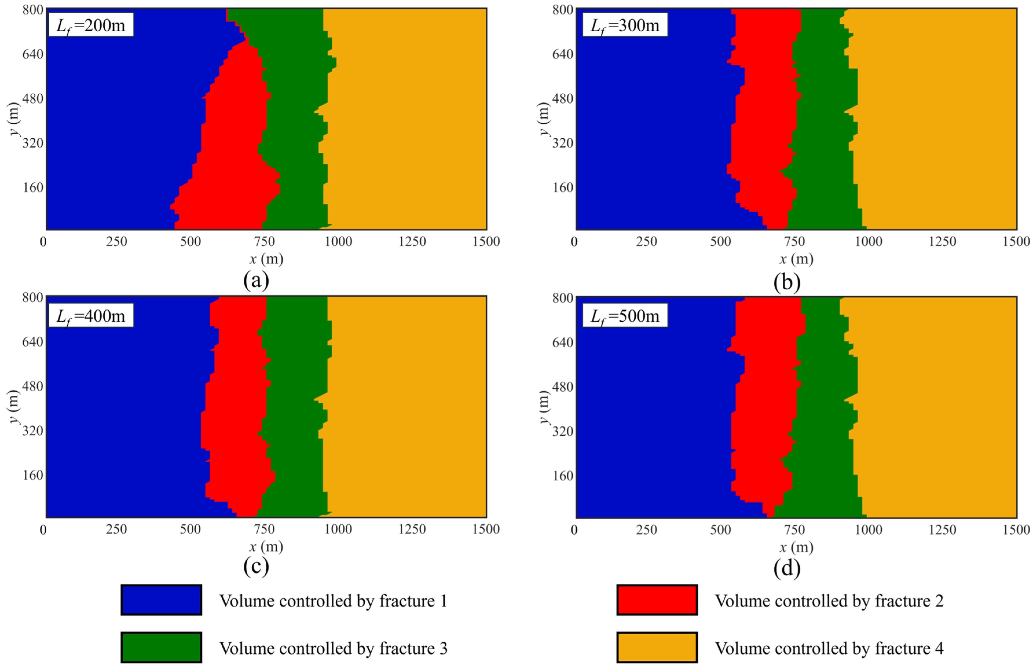
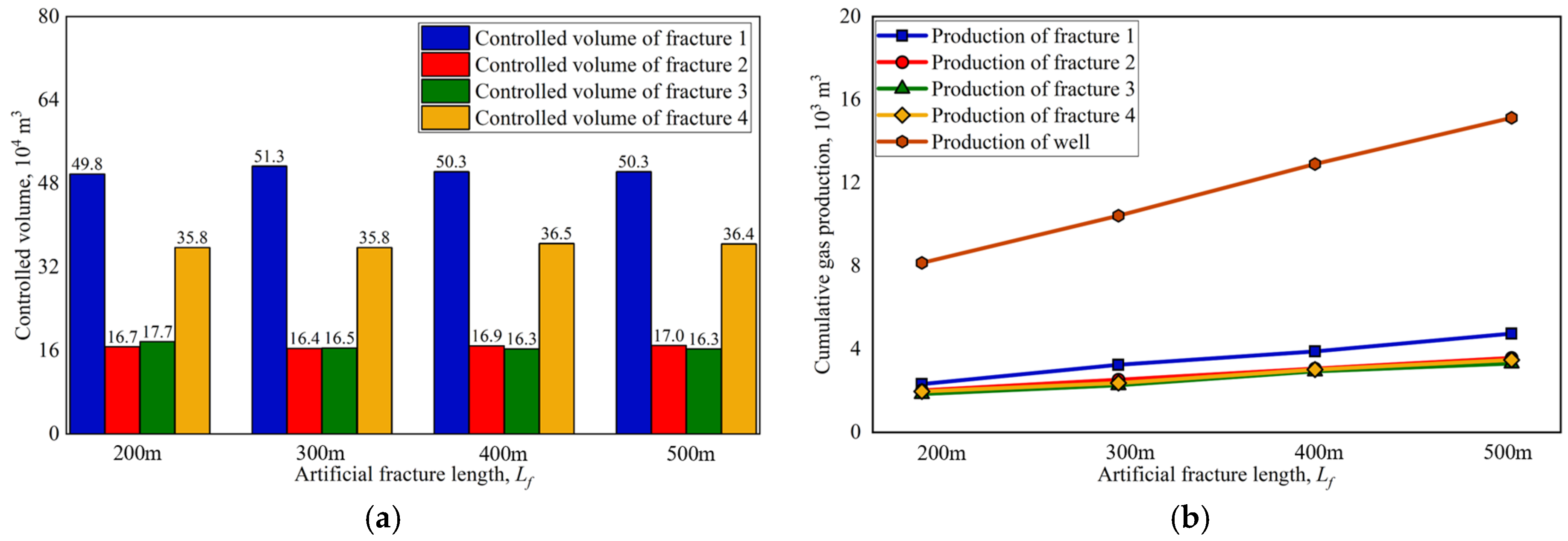
4.2. Artificial Fracture Length

A series of artificial fracture lengths, ranging from 200 m to 500 m, is used to study its impact on both the control volumes and production performance of each artificial fracture, as well as on the well productivity. Figure 7 illustrates the distribution of the controlled volume of each artificial fracture with varying artificial fracture lengths. As depicted in the figure, when the artificial fracture length is small, the distribution of controlled volumes shows noticeable changes as the fracture length increases. However, as the fracture length continues to increase, the distribution of controlled volumes stabilizes and becomes less sensitive to further increases in fracture length. Despite these initial changes in distribution, the total controlled volume for each fracture remains nearly constant across different fracture lengths, as shown in Figure 8a. This suggests that while the fracture length influences the spatial distribution of controlled volumes, it does not significantly alter the overall controlled volume for each fracture. Figure 8b compares the cumulative gas production of each fracture and the well, with different artificial fracture lengths (calculated by Equation (9)). As the fracture length increases, the cumulative production of the well increases significantly. This is primarily driven by the increase in fracture length, which enhances connection with a larger portion of the reservoir, allowing more reservoir area to contribute to production. Although the controlled volumes for each fracture remain almost unchanged, as shown in Figure 8a, longer fractures effectively connect more regions of the reservoir, leading to higher cumulative gas production. Specifically, the cumulative gas production from the well increases from approximately 8.15 × 10³ m3 at Lf = 200 m to 1.51 × 10⁴ m3 at Lf = 500 m, corresponding to an approximate 85.27% increase.

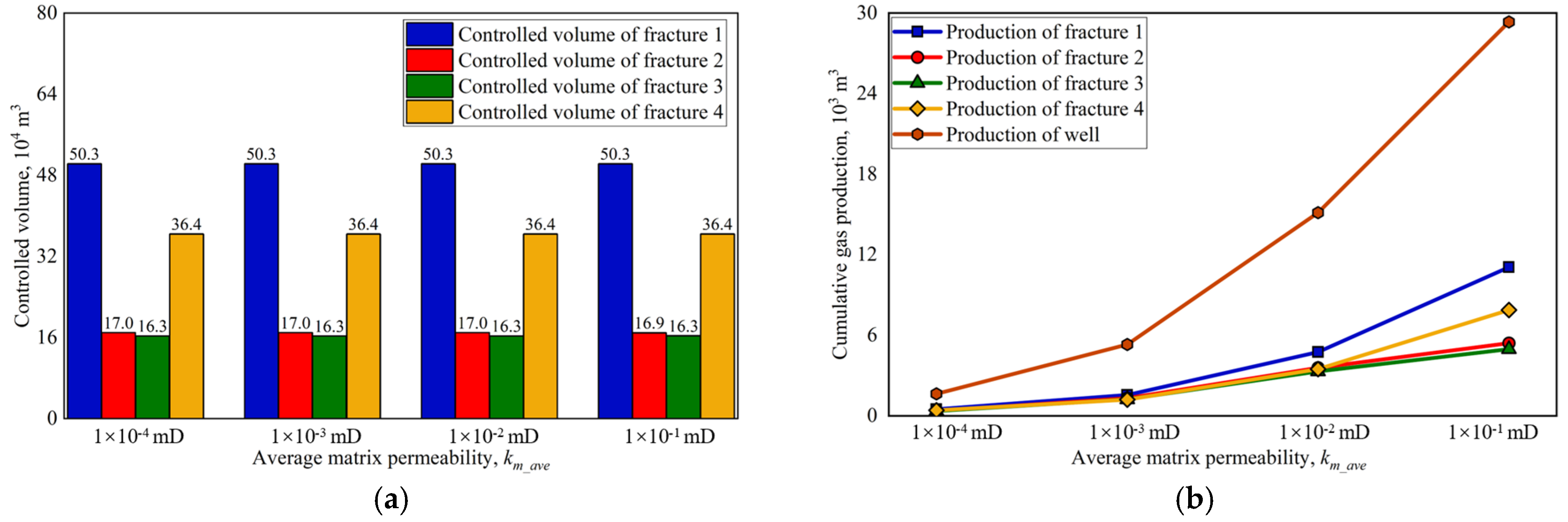
4.3. Average Matrix Permeability

The average matrix permeability is varied from 1 × 10⁻⁴ mD to 1 × 10⁻¹ mD (i.e., the average matrix permeability in the x and y directions) to investigate its impact on both the control volumes and production performance of each artificial fracture, as well as on the well productivity. These values are based on previously generated random values of the benchmark shale gas reservoir model, scaled by a multiplier. Figure 9 illustrates the distribution of the controlled volume of each artificial fracture with different average matrix permeabilities. It can be observed that the distribution of volumes controlled by each fracture remains consistent across these varying permeability conditions. This is attributed to the fact that changes in the average matrix permeability predominantly affect the fluid flow capacity within the entire reservoir. However, this alteration does not significantly impact the volume controlled by each artificial fracture, which is primarily determined by the fracture geometry and connectivity. This trend is confirmed by Figure 10a, which compares the controlled volume of each artificial fracture across different average matrix permeabilities. As seen in the figure, the total controlled volume for each fracture remains nearly constant, regardless of the changes in matrix permeability. Figure 10b further investigates the cumulative gas production from each artificial fracture and the well with different average matrix permeabilities (calculated by Equation (9)). The results show that, as the average matrix permeability increases, the cumulative gas production from fracture 1 (blue dotted line) and fracture 4 (yellow dotted line) increases significantly, while the production from fractures 2 (red dotted line) and 3 (green dotted line) rises at a slower rate. This aligns with the previous observation that the volumes controlled by fractures 1 and 4 are more substantial, leading to higher production. In contrast, fractures 2 and 3, which have smaller controlled volumes, show a less-pronounced increase in production. These findings indicate that although the controlled volumes are stable across different permeability conditions, the matrix permeability does impact the flow rate and ultimately the cumulative production from fractures, especially for fractures with larger volumes. Notably, as the average matrix permeability increases from 1 × 10⁻⁴ mD to 1 × 10⁻¹ mD, the cumulative gas production from the well increases from approximately 1.64 × 10³ m3 to 2.9 × 10⁴ m3, representing an increase of about 16.7 times.

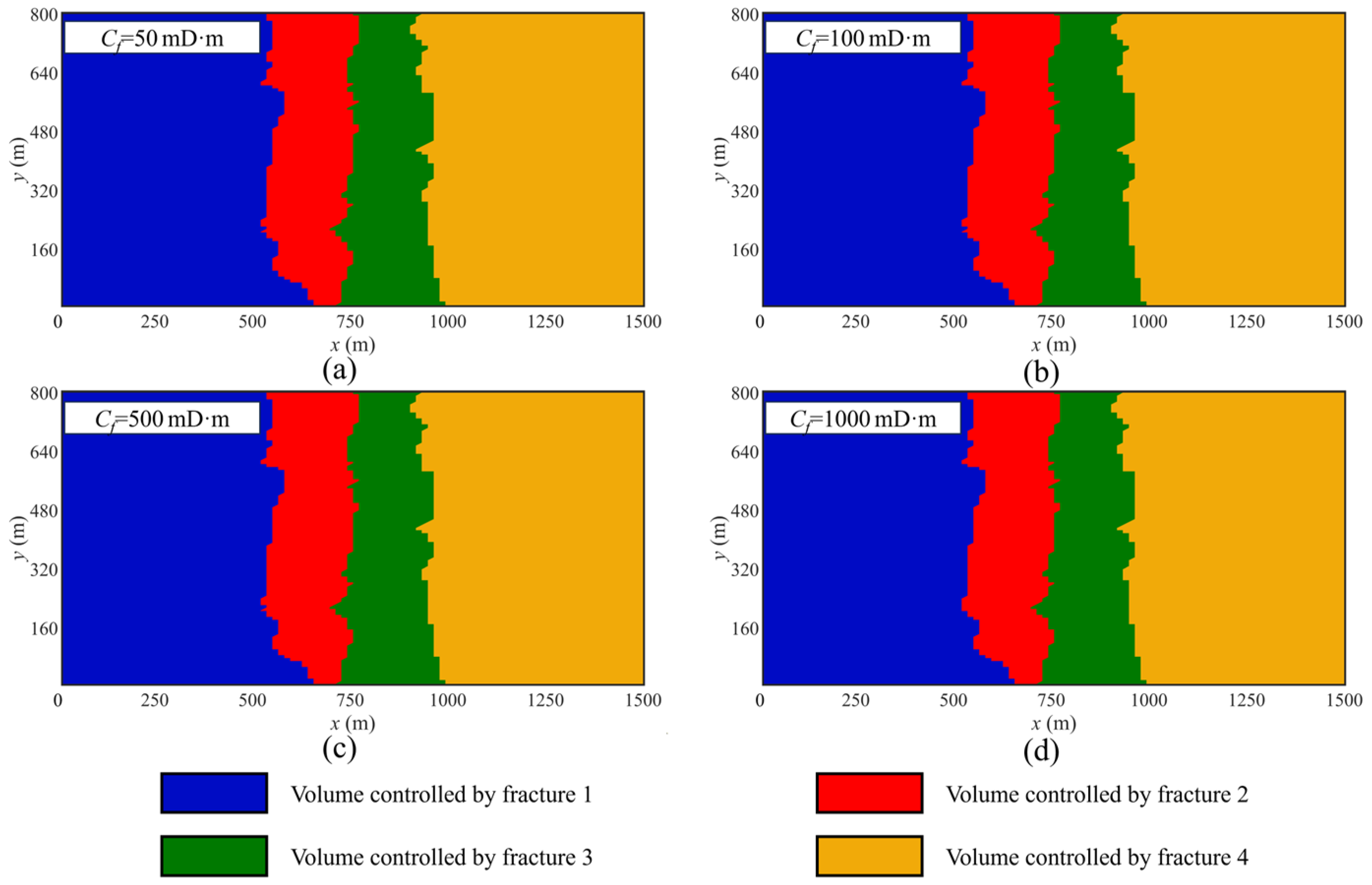
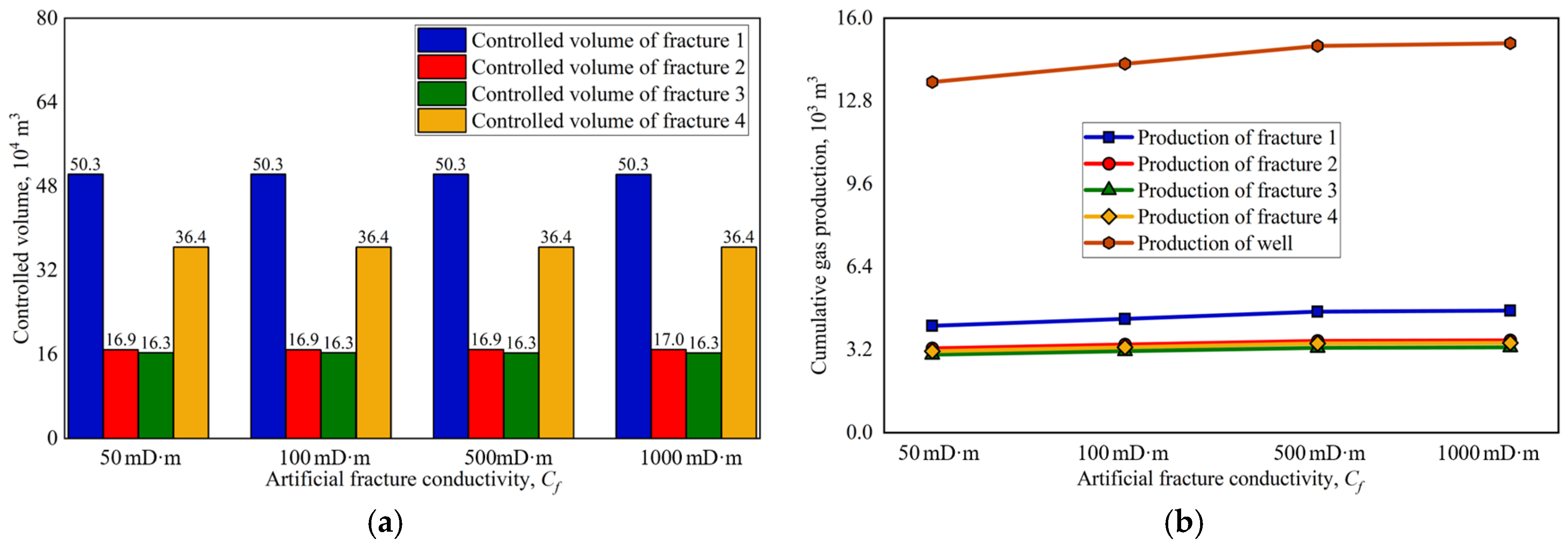
4.4. Artificial Fracture Conductivity

A series of artificial fracture conductivities, ranging from 50 mD·m to 1000 mD·m, is used to study its impact on both the control volumes and production performance of each artificial fracture, as well as on the well productivity. Figure 11 shows the distribution of the controlled volume of each artificial fracture with varying artificial fracture conductivities. It can be observed that the controlled volume distribution remains consistent despite variations in fracture conductivity. This consistency is mainly because the fracture conductivity primarily affects the fluid transport efficiency along the fractures, while fluid flow in regions far from the fractures is mainly influenced by the properties of the matrix and natural fractures. This observation is further supported by Figure 12a, which compares the controlled volume of each fracture under different fracture conductivities. This figure indicates that the controlled volume of each fracture remains nearly unchanged as the fracture conductivity increases. Figure 12b presents the cumulative gas production from each fracture and the well under varying fracture conductivity. It can be observed that the cumulative production from the well significantly increases with higher fracture conductivity, indicating enhanced fluid transport and reduced flow resistance within the fracture network. Specifically, the cumulative gas production from the well increases from approximately 1.35 × 10⁴ m3 at Cf = 50 mD·m to 1.5 × 10⁴ m3 at Cf = 1000 mD·m, corresponding to an approximate 11.11% increase.

5. Conclusions

In this work, based on the concept of DTOF, the authors propose a fast simulation method to efficiently simulate the production behavior of each artificial fracture throughout the shale gas reservoir production process. The method utilizes the fast marching method (FMM) to solve the Eikonal equation, enabling efficient calculation of controlled volumes and production of individual fractures. According to the obtained results in this work, the authors provide the following conclusions:
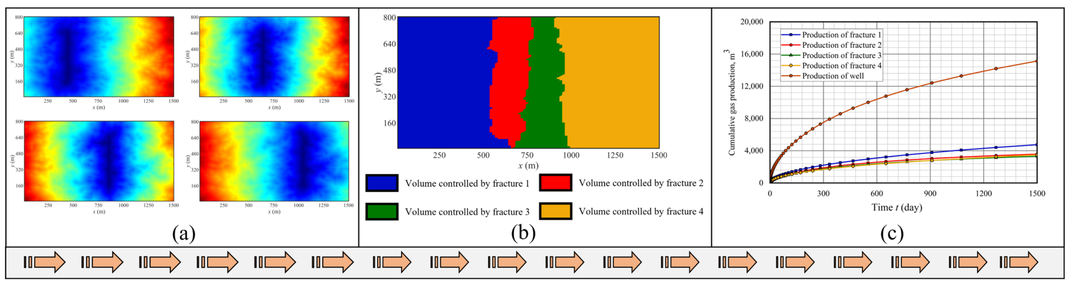
  • The proposed method provides a computationally efficient approach to simulate the production behavior of each artificial fracture in shale gas reservoirs without simulating the production process of the entire reservoir.
  • The controlled volume directly determines the production of each artificial fracture, with a greater controlled volume leading to higher gas production.
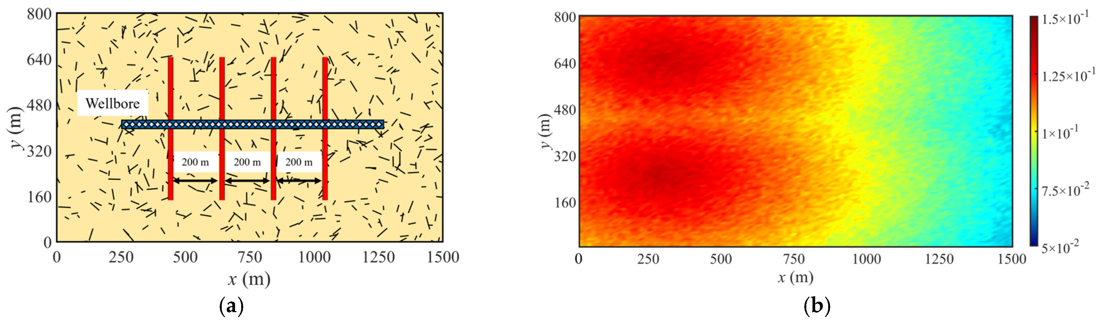
  • Fracture parameters, including the length and spacing of artificial fractures, significantly influence the distribution and volume of the controlled area for each fracture within the reservoir, thereby affecting the production performance of artificial fractures. In contrast, the conductivity of artificial fractures has little impact on the distribution and volume of the controlled area but plays a crucial role in enhancing production performance. Specifically, longer artificial fractures, wider fracture spacing, and higher fracture conductivity result in increased gas production from the gas well.
  • The matrix permeability has a minimal impact on the distribution of the controlled volume of artificial fractures, but it significantly influences the gas production from these fractures. Specifically, a higher matrix permeability leads to increased production from artificial fractures, especially those with large, controlled volumes.

Author Contributions

Conceptualization, X.Y. and Q.L.; methodology, X.Y.; software, C.C.; validation, C.C. and D.D.; formal analysis, H.H. and S.L.; investigation, X.Y., C.C. and D.D.; resources, X.Y. and Y.C.; data curation, X.Y.; writing—original draft preparation, X.Y.; writing—review and editing, X.Y. and Y.C.; visualization, X.Y., C.C. and D.D.; supervision, Q.L. and B.T.; project administration, Q.L. and B.T.; funding acquisition, Q.L. and B.T. All authors have read and agreed to the published version of the manuscript.

Funding

This research was funded by “National Natural Science Foundation of China” (No. 52474051).

Data Availability Statement

The original contributions presented in this study are included in the article. Further inquiries can be directed to the corresponding authors.

Conflicts of Interest

Authors Xuefeng Yang, Cheng Chang, Dan Dai, Haoran Hu, Shengwang Lin and Yizhao Chen were employed by the PetroChina Southwest Oil & Gas Field Company. The remaining authors declare that the research was conducted in the absence of any commercial or financial relationships that could be construed as a potential conflict of interest.

Nomenclature

Aflow area
Bvolume factor
cttotal compressibility
Llength
ppressure
ttime
Treservoir temperature
tfpseudo-front time
Zcompressibility factor
ρggas density
vflow rate
Vpdrainage volume
ϕporosity
μggas viscosity
βtime conversion factor
qmgas mass flow rate
qrproduction mass rate
qDdimensionless mass flow rate
rthe distance from the wellbore
Subscripts and superscripts
afartificial fracture
iinitial state
nfnatural fracture
pnnormalized pseudo
wfwellbore
sspacing
scunder standard conditions

Appendix A

The gas mass flow rate under normalized pseudo-time can be described using Darcy’s law [23]:
q m r , t p n = ρ g k A r μ g p r , t p n r
where ρg is gas density, qm is gas mass flow rate, r is the distance from the wellbore, tpn is normalized pseudo-time, k is permeability, A is flow area, μg is gas viscosity, and p is pressure.
Incorporating Equation (A1) with Equation (3), we can obtain the gas mass flow under normalized pseudo-pressure:
q m , p n = p M Z p R T k A r μ g p r , t p n r = α k A r p p n r , t p n r ,      α = p μ g Z i M R T
where ρg = PM/(ZRT), M, Z, and R are the gas molar mass, compressibility factor, and universal gas constant, respectively. T is the reservoir temperature, and α is a constant factor. The drainage volume can be represented as
d V p = ϕ A r d r
where Vp is drainage volume. From Equation (A3) and the chain rule, we can obtain
r = V p d V p d r = V p ϕ A r
Inserting Equations (A3) and (A4) into Equation (A2), we can obtain the mass flow rate of gas with drainage volume as the spatial coordinate:
q m , p n V p , t p n = α k ϕ A 2 p V p , t p n V p ,      α = p μ g Z i M R T
The Darcy flow of gas in the drainage volume coordinate can be approximated by multiplying the production mass flow rate at the wellbore by a dimensionless mass flow rate [29]. Based on this approximation, the Equation (A5) can be written as
q m , p n V p , t p n q r , m t p n q D , m V p , t p n
where qr and qD are the production mass rate and dimensionless mass flow rate, respectively. Combining Equations (A5) and (A6), and integrating with respect to pressure and drainage volume, yield
Δ p p n = p p n , i p p n , w f = q r , m t p n β 0 V p t p n q D , m V , t p n k ϕ A 2 d V
where pi and pwf are the initial reservoir pressure and wellbore pressure, respectively, and V is the specific volume within the drainage volume. It should be noted that when calculating the production of a gas well with geometric approximation using the drainage volume coordinate, the flow within the drainage volume is assumed to be pseudo-steady-state flow, while the flow beyond the drainage volume is considered negligible [19,30]. In this approach, the viscosity, permeability, and porosity in the Equation (A7) represent the average values over the entire drainage volume. Inserting Equations (A3) and (A6) into the continuity equation (Equation (1)), the continuity equation can be rewritten as
p p n t p n = q r , m q D , m V p V p 1 ρ g c t i
Under pseudo-steady-state conditions, the left side of Equation (A4) is constant, which implies a linear relationship between the dimensionless flow rate qD and drainage volume Vp on the right-hand side of the equation. This relationship can be expressed as
q D , m V , t p n = a V + b
where V is the specific volume within the drainage volume. Based on the flow assumptions outlined earlier, the gas mass flow rate is equal to the production mass flow rate at the wellbore, qm,pn (0, t) = qr,m (t), and the gas mass flow rate is 0 at the drainage volume boundary, qm,pn (Vp, t) = 0. Incorporating the two boundary conditions into Equations (A6) and (A9) yields
q D , m V , t p n = 1 V V p ( t p n )
Inserting Equation (A10) into Equation (A7), we have
q r , m t p n = Δ p p n β 1 0 V p t p n 1 k ϕ A 2 1 V V p ( t p n ) d V ,      β = p μ g Z i M R T
By dividing Equation (A11) by the gas density, the gas production rate can be obtained:
q r t p n = q r , m ρ g = Δ p p n β ρ g 1 0 V p t p n 1 k ϕ A 2 1 V V p ( t p n ) d V ,      β = p μ g Z i M R T
The qr in Equation (A11) refers to the gas production rate under the reservoir conditions, which needs to be converted to the standard conditions by dividing by the volume factor:
q r t p n = Δ p p n β ρ g B 1 0 V p t p n 1 k ϕ A 2 1 V V p ( t p n ) d V = T s c T p s c p μ g Z i p ¯ p n p p n , w f 0 V p t p n 1 k ϕ A 2 1 V V p ( t p n ) d V
where B is the volume factor, which is defined as
B = p s c T s c Z s c Z T p
where psc, Tsc, and Zsc are pressure, temperature, and compressibility factor under standard conditions, respectively. Zsc is typically taken as 1 under standard conditions.
To calculate the gas production rate, it is essential to determine the average pseudo-pressure of the drainage volume p n ¯ . Combining Equations (A8) and (A10) and integrating, we obtain the equation to calculate the pressure at a location within the reservoir:
p p n ( V p , t p n ) = p p n , i t p n ( V p ) t p n q r , m t p n ρ g c t i V p d t p n
where tpn(vp) is pseudo-time corresponding to the propagation of the pseudo-pressure front at the specified location, and the integral begins at the time the pseudo-pressure front reaches that location.
The average pseudo-pressure of the drainage volume is obtained by integrating the pseudo-pressure at each location in the drainage volume and dividing by the drainage volume, which is defined as
p ¯ p n = 1 V p t p n 0 V p t p n p p n ( V , t p n ) d V
where V is specific volume within the drainage volume.

References

  1. Omari, A.; Wang, C.; Li, Y.; Xu, X. The progress of enhanced gas recovery (EGR) in shale gas reservoirs: A review of theory, experiments, and simulations. J. Pet. Sci. Eng. 2022, 213, 110461. [Google Scholar] [CrossRef]
  2. Hu, P.; Geng, S.; Liu, X.; Li, C.; Zhu, R.; He, X. A three-dimensional numerical pressure transient analysis model for fractured horizontal wells in shale gas reservoirs. J. Hydrol. 2023, 620, 129545. [Google Scholar] [CrossRef]
  3. Jiang, C.; Lu, T.; Zhang, D.; Li, G.; Duan, M.; Chen, Y.; Liu, C. An experimental study of deformation and fracture characteristics of shale with pore-water pressure and under triaxial cyclic loading. R. Soc. Open Sci. 2018, 5, 180670. [Google Scholar] [CrossRef] [PubMed]
  4. Zhang, T.; Sun, S.; Song, H. Flow mechanism and simulation approaches for shale gas reservoirs: A review. Transp. Porous Media 2019, 126, 655–681. [Google Scholar] [CrossRef]
  5. Iferobia, C.C.; Ahmad, M. A review on the experimental techniques and applications in the geomechanical evaluation of shale gas reservoirs. J. Nat. Gas Sci. Eng. 2020, 74, 103090. [Google Scholar] [CrossRef]
  6. Ren, L.; Lin, R.; Zhao, J. Stimulated reservoir volume estimation and analysis of hydraulic fracturing in shale gas reservoir. Arabian J. Sci. Eng. 2018, 43, 6429–6444. [Google Scholar] [CrossRef]
  7. Zhang, H.; Sheng, J. Optimization of horizontal well fracturing in shale gas reservoir based on stimulated reservoir volume. J. Pet. Sci. Eng. 2020, 190, 107059. [Google Scholar] [CrossRef]
  8. Hou, P.; Liang, X.; Zhang, Y.; He, J.; Gao, F.; Liu, J. 3D multi-scale reconstruction of fractured shale and influence of fracture morphology on shale gas flow. Nat. Resour. Res. 2021, 30, 2463–2481. [Google Scholar] [CrossRef]
  9. Rahmanifard, H.; Plaksina, T. Application of fast analytical approach and AI optimization techniques to hydraulic fracture stage placement in shale gas reservoirs. J. Nat. Gas Sci. Eng. 2018, 52, 367–378. [Google Scholar] [CrossRef]
  10. Wang, L.; Yao, Y.; Zhao, G.; Adenutsi, C.D.; Wang, W.; Lai, F. A hybrid surrogate-assisted integrated optimization of horizontal well spacing and hydraulic fracture stage placement in naturally fractured shale gas reservoir. J. Pet. Sci. Eng. 2022, 216, 110842. [Google Scholar] [CrossRef]
  11. Xu, Y.; Cavalcante Filho, J.S.; Yu, W.; Sepehrnoori, K. Discrete-fracture modeling of complex hydraulic-fracture geometries in reservoir simulators. SPE Reserv. Eval. Eng. 2017, 20, 403–422. [Google Scholar]
  12. Hosseini, S.A.; Kang, S.; Datta-Gupta, A. Qualitative well placement and drainage volume calculations based on diffusive time of flight. J. Pet. Sci. Eng. 2010, 75, 178–188. [Google Scholar] [CrossRef]
  13. Datta-Gupta, A.; Xie, J.; Gupta, N.; King, M.J.; Lee, W.J. Radius of investigation and its generalization to unconventional reservoirs. J. Pet. Technol. 2011, 63, 52–55. [Google Scholar] [CrossRef]
  14. Sethian, J.A. A fast marching level set method for monotonically advancing fronts. Proc. Natl. Acad. Sci. USA 1996, 93, 1591–1595. [Google Scholar]
  15. Zhang, Y.; Bansal, N.; Fujita, Y.; Datta-Gupta, A.; King, M.J.; Sankaran, S. From streamlines to fast marching: Rapid simulation and performance assessment of shale gas reservoirs using diffusive time of flight as a spatial coordinate. In Proceedings of the SPE Unconventional Resources Conference, The Woodlands, TX, USA, 1–3 April 2014. Paper SPE-168997. [Google Scholar]
  16. Teng, B. Simulation model size reduction using volume of investigation by fast marching method. J. Pet. Sci. Eng. 2020, 191, 107183. [Google Scholar]
  17. Lu, C.; Chen, L.; Wang, X.; Luo, W.; Peng, Y.; Cui, Y.; Wang, L.; Teng, B. A New Approach for Determining the Control Volumes of Production Wells considering Irregular Well Distribution and Heterogeneous Reservoir Properties. Geofluids 2021, 2021, 6666831. [Google Scholar]
  18. Chen, H.; Li, A.; Terada, K.; Datta-Gupta, A. Rapid simulation of unconventional reservoirs by multidomain multiresolution modeling based on the diffusive time of flight. SPE J. 2023, 28, 1083–1096. [Google Scholar] [CrossRef]
  19. Zhang, Y.; Yang, C.; King, M.J.; Datta-Gupta, A. Fast-marching methods for complex grids and anisotropic permeabilities: Application to unconventional reservoirs. Paper SPE-163637. In Proceedings of the SPE Reservoir Simulation Symposium, The Woodlands, TX, USA, 18–20 February 2013. [Google Scholar]
  20. Fujita, Y.; Datta-Gupta, A.; King, M.J. A comprehensive reservoir simulator for unconventional reservoirs that is based on the Fast Marching method and diffusive time of flight. SPE J. 2016, 21, 2276–2288. [Google Scholar]
  21. Iino, A.; Jung, H.Y.; Onishi, T.; Datta-Gupta, A. Rapid simulation accounting for well interference in unconventional reservoirs using fast marching method. Paper URTEC-2020-2468-MS. In Proceedings of the SPE/AAPG/SEG Unconventional Resources Technology Conference, Virtual, 20–22 July 2020. [Google Scholar]
  22. Al-Hussainy, R.; Ramey, H.J., Jr.; Crawford, P.B. The flow of real gases through porous media. J. Pet. Technol. 1966, 18, 624–636. [Google Scholar]
  23. Darcy, H. Dalmont; Les Fontaines Publiques De La Ville De Dijon: Paris, France, 1856. [Google Scholar]
  24. Lee, W.J.; Holditch, S.A. Application of pseudotime to buildup test analysis of low-permeability gas wells with long-duration wellbore storage distortion. J. Pet. Technol. 1982, 34, 2877–2887. [Google Scholar]
  25. Xie, J.; Yang, C.; Gupta, N.; King, M.J.; Datta-Gupta, A. Depth of investigation and depletion in unconventional reservoirs with fast-marching methods. SPE J. 2015, 20, 831–841. [Google Scholar] [CrossRef]
  26. Kim, J.U.; Datta-Gupta, A.; Brouwer, R.; Haynes, B. Calibration of high-resolution reservoir models using transient pressure data. Paper SPE-124834-MS. In Proceedings of the SPE Annual Technical Conference and Exhibition, New Orleans, LO, USA, 4–7 October 2009. [Google Scholar]
  27. Zeng, H.; Fan, D.; Yao, J.; Sun, H. Pressure and rate transient analysis of composite shale gas reservoirs considering multiple mechanisms. J. Nat. Gas Sci. Eng. 2015, 27, 914–925. [Google Scholar] [CrossRef]
  28. Zeng, F.; Peng, F.; Guo, J.; Xiang, J.; Wang, Q.; Zhen, J. A transient productivity model of fractured wells in shale reservoirs based on the succession pseudo-steady state method. Energies 2018, 11, 2335. [Google Scholar] [CrossRef]
  29. Winestock, A.; Colpitts, G.P. Advances in estimating gas well deliverability. J. Can. Pet. Technol. 1965, 4, 111–119. [Google Scholar]
  30. Agarwal, R.G. Direct method of estimating average reservoir pressure for flowing oil and gas wells. Paper SPE-135804-MS. In Proceedings of the SPE Annual Technical Conference and Exhibition, Florence, Italy, 19–22 September 2010. [Google Scholar]
Figure 1. Schematic of the framework for gas production calculation using the proposed method: (a) pseudo-front time distribution of each artificial fracture, (b) control volume distribution, and (c) production calculation.
Processes 13 00984 g001
Figure 2. Illustration of 2D shale gas reservoir model and comparison of the simulated result: (a) 2D shale gas reservoir model and (b) comparison of gas production rate from Eclipse and the proposed method.
Processes 13 00984 g002
Figure 3. Benchmark shale gas reservoir model and its porosity distribution: (a) illustration of the benchmark reservoir model with artificial and natural fractures, (b) porosity distribution.
Processes 13 00984 g003
Figure 4. Permeability distribution of the shale gas reservoir: (a) permeability distribution along the x-direction and (b) permeability distribution along the y-direction.
Processes 13 00984 g004
Figure 5. Distribution of the controlled volume of each artificial fracture with different artificial fracture spacing: (a) Ls = 50 m, (b) Ls = 100 m, (c) Ls = 200 m, and (d) Ls = 400 m.
Processes 13 00984 g005
Figure 6. Comparison of controlled volume and cumulative production of each artificial fracture with different artificial fracture spacing: (a) controlled volume and (b) cumulative gas production.
Processes 13 00984 g006
Figure 7. Distribution of the controlled volume of each artificial fracture with different artificial fracture lengths: (a) Lf = 200 m, (b) Lf = 300 m, (c) Lf = 400 m, and (d) Lf = 500 m.
Processes 13 00984 g007
Figure 8. Comparison of controlled volume and cumulative production of each artificial fracture with different artificial fracture lengths: (a) controlled volume and (b) cumulative gas production.
Processes 13 00984 g008
Figure 9. Distribution of the controlled volume of each artificial fracture with different average matrix permeabilities: (a) km_ave = 1 × 10⁻⁴ mD, (b) km_ave = 1 × 10⁻³ mD, (c) km_ave = 1 × 10⁻² mD, and (d) km_ave = 1 × 10⁻¹ mD.
Processes 13 00984 g009
Figure 10. Comparison of controlled volume and cumulative production of each artificial fracture with different average matrix permeabilities: (a) controlled volume and (b) cumulative gas production.
Processes 13 00984 g010
Figure 11. Distribution of the controlled volume of each artificial fracture with different artificial fracture conductivities: (a) Cf = 50 mD·m, (b) Cf = 100 mD·m, (c) Cf = 500 mD·m, and (d) Cf = 1000 mD·m.
Processes 13 00984 g011
Figure 12. Comparison of controlled volume and cumulative production of each artificial fracture with different artificial fracture conductivities: (a) controlled volume and (b) cumulative gas production.
Processes 13 00984 g012
Table 1. Values of the other parameters applied in the benchmark shale gas reservoir model.
PropertyValuePropertyValue
Initial reservoir pressure pini (MPa)25Wellbore pressure pw (MPa)5
Temperature of the reservoir T (°C)125Gas molar mass Mmg (g/mol)16
Permeability of artificial fracture kaf (mD)1 × 10⁶Permeability of natural fracture knf (mD)1 × 10⁴
Porosity of artificial fracture ϕaf0.5Porosity of natural fracture ϕnf0.8
Disclaimer/Publisher’s Note: The statements, opinions and data contained in all publications are solely those of the individual author(s) and contributor(s) and not of MDPI and/or the editor(s). MDPI and/or the editor(s) disclaim responsibility for any injury to people or property resulting from any ideas, methods, instructions or products referred to in the content.

