Data-Driven Model for Cyclic Tasks of Robotic Systems: Study of the Repeatability Conditions

Abstract

Ensuring repeatability in robotic manipulators is critical for industrial applications, particularly in cyclic tasks where precision and consistency are required. This study aims to establish the conditions that are necessary for repeatability in data-driven task-space control, compare repeatability across redundant robotic manipulators, and reduce the computational costs associated with data-based control methods compared to traditional model-based approaches. To achieve this, a large number of cyclic actions are simulated, mimicking real-world industrial routines. The methodology evaluates the estimated Jacobian matrix’s manipulability and its role in facilitating effective task execution within the operational space of the robot. The results demonstrate that the proposed approach achieves consistent repeatability at the full pose level of the end-effector, integrating both position and orientation. In particular, the findings indicate that the proposed controller minimizes variability and ensures reliable motion execution, even in the presence of system redundancies, as observed in the eight-DoF KUKA YouBot manipulator. These insights contribute to advancing data-driven control strategies for redundant robotic systems, enhancing their applicability in industrial settings.

1. Introduction

Robotic manipulators perform commonly repetitive tasks autonomously in current industrial environments, reducing human participation. This technology increases manufacturing precision and consistency, improves efficiency, and reduces errors [1]. It also frees human workers to focus on intricate and innovative tasks, improving safety and job satisfaction. Consequently, it is imperative that these robotic systems perform tasks both precisely and efficiently [2,3]. On the other hand, redundant robots, which have extra degrees of freedom (DoFs) beyond the task requirement, generally more than six, enhance flexibility and adjustability, particularly when mobile bases are used [4]. This feature enables multiple task executions, path optimization, and obstacle avoidance, contributing to precise positioning in challenging settings [5,6]. However, increasing DoFs increases the complexity of control and repeatability issues as variations in joint configurations and execution paths may obstruct uniform performance in repetitive tasks, potentially leading to cumulative errors that affect the precision and reliability of automated systems.

There is a trade-off between robots with limited degrees of freedom (DoFs), which excel in repeatability and precision for repetitive tasks, and redundant robots, which provide enhanced flexibility and reach at the expense of consistency in repetitive operations. The repeatability issues in redundant robots arise from their multiple possible configurations for the same task [7]. Quadratic programming is used to enhance task accuracy by minimizing errors, but this approach relies heavily on theoretical models [8]. Differences between these models and actual conditions may cause deviations. Even if the error at the end-effector is reduced, slight configuration changes can accumulate over time, affecting long-term precision and performance.

In the last ten years, data-driven modeling and control (DDMC) has become a key approach to improving autonomy in industrial systems [9]. It uses real-time data in closed-loop systems with sensors, actuators, and processors. In DDMC, efficiency involves minimizing hardware, such as encoders. It operates on feedback from the end-effector’s position, reducing reliance on multiple measurement sources and thus lowering the failure risk. DDMC offers a cutting-edge solution for the precise control of the 3D coordinates of the end-effector in industrial tasks, previously managed by fully specified analytical models [10]. DDMC requires only the correlation of outputs with inputs in unknown robotic systems, making it versatile for various types of robots, including rigid, soft, inertial, and non-inertial [11,12,13,14].

DDMC strategies are increasingly popular as they circumvent the constraints of model-based methods by using sensor data to predict system performance [9,15,16,17,18,19]. For example, Ref. [20] showcased a dual-arm robotic system executing grasping tasks without pre-existing kinematic or dynamic knowledge. This method ensured high repeatability due to constrained end-effectors but did not tackle issues of redundancy. With increased redundancy, disturbances and model inaccuracies are amplified, notably in mobile manipulators.

For a robotic arm, the joint velocity acts as the input, and the end-effector velocity serves as the output [19]. This connection allows for online estimation of the Jacobian matrix without a predefined model, which is crucial in the robot kinematic model, especially for closed-loop control within the task-space of the end-effector. In robotic systems using DDMC, there are typically two phases. Initially, the Jacobian matrix is computed online via an estimation method. For example, the work of [21] used an adaptive Kalman filter to estimate the Jacobian for trajectory tracking in a continuum robot, while Ref. [19] estimated it for an eight-DoF robot using the Pseudo Jacobian Matrix (PJM) algorithm. The second phase is the design of a control law in task-space using end-effector pose feedback and applying the inverse of the estimated Jacobian to convert control signals into joint coordinates. The closed-loop system presumes an equivalent inverse relationship between inputs and outputs; thus, model estimation errors must converge before control errors in the closed-loop system can be resolved. Failing this could compromise end-effector operations. The work in Ref. [22] proposed a novel DDMC for developing a complete pose (position and orientation) control strategy for the end-effector of a manipulator. The innovation of this work lies in the ability to estimate an equivalent analytical Jacobian matrix without the need to parameterize the orientation partition using a specific orientation representation, as is typically required in model-dependent control schemes. This alleviates the singularity-related issues that typically complicate orientation control algorithms. This offers greater flexibility in implementation as changes in orientation representation do not require offline modifications of the algorithm.

Real robotic systems face intensified challenges when sensor data are integrated with theoretical models. As noted in Ref. [23], sensor error, noise, disturbances, and unmodeled dynamics hinder control. Accurate position measurements in the operational space are difficult, particularly under uncertainty [24,25]. Torque-mode robots often encounter modeling errors despite accurate sensors [26]. The work in Ref. [27] used a nonlinear disturbance observer to mitigate unmodeled nonlinearities in a two-link torque-mode robot, managing modeling issues to maintain stability and precision. Robust adaptive controls have also been proposed to handle disturbances, such as in [28,29,30,31,32].

The repeatability of redundant robots was first examined by the authors in [33], who defined it using exterior derivatives to assess the integrability of differential constraints. The authors of Ref. [34] expanded on this, using differential geometry to determine the repeatability conditions and formulating a matching control strategy. The authors of Ref. [35] progressed by using redundancy to create repeatable inverses of augmented Jacobian matrices, selecting the appropriate null spaces. Similarly, the authors of Ref. [36] leveraged redundancy for secondary tasks in the joint-space, aligning repeatable joint-space trajectories with primary tasks to achieve cyclic kinematic control. The study in Ref. [37] furthered these concepts by crafting repeatable joint-space tasks using periodicity and repeatability metrics. The authors of Ref. [38] applied differential geometry, notably exterior derivatives, for improved path planning. Furthermore, the study in Ref. [39] proposed an optimization approach to generate repeatable joint-space trajectories through holonomic loops for pseudoinverse control.

The pursuit of cyclic motion in redundant robots requires motion planning to address repeatability concerns, as highlighted in [40]. The authors pointed out the critical role of offline motion planning for predefined repetitive tasks. In response, the authors of Ref. [41] developed a randomized planner to create cyclic collision-free paths within the configuration space, integrating it with their control strategy. The study in Ref. [42] synthesized these advancements by reviewing previous studies on repeatability and suggested motion-planning-based remedies. In more recent research, the work in Ref. [43] unveiled a repetitive motion planning method that is suitable for pseudoinverse-based control systems in redundant robots, taking into account joint constraints, thereby underscoring the value of motion planners for managing redundancy and maintaining repeatability. Furthermore, the authors of Ref. [42] noted the drawbacks of conventional kinematic controls, mainly their lack of backtracking ability. These techniques often result in locally optimal solutions without considering past outcomes or anticipating future actions, making them prone to producing reactive motion, where robot movements adapt in real time to current dynamics, complicating repeatability in tasks demanding consistency.

In this research, it is demonstrated that computing the forward and inverse kinematics, using DDMC strategies, significantly improves the repeatability of holonomic redundant robots, such as omnidirectional mobile manipulators, when controlled in the task-space, and without the need of implicitly enforcing repeatability through secondary tasks or path-planning. In order to demonstrate this, it is necessary to first analyze the conditions that are necessary for repeatability and its relationship to the integrability of dynamic systems according to the Frobenius theorem. By considering these conditions, it becomes understandable that some dynamic systems are inherently non-integrable, such as rotational systems, or those closed-loop systems where the map between inputs/outputs is nonlinear, aspects that are always present in redundant mobile manipulators, making them inherently non-integrable. Therefore, in this work, the integrability conditions are summarized such that it becomes clear how the DDMC strategy makes a redundant mobile manipulator system fulfill such conditions, even if it is inherently non-integrable.

The proposed DDMC strategy uses the update law from [22] to estimate the Jacobian matrix and also incorporates a Sherman–Morrison update to compute the pseudoinverse of the Jacobian matrix. Both update laws are known to be rank-1, which means the Jacobian and its inverse are updated through the exterior product of two vectors, forming a matrix of rank-1; this results in a significantly more efficient way to derive forward and inverse kinematics compared to classical model-based methods that require the explicit inversion of the Jacobian matrix. Therefore, our DDMC strategy led to faster convergence of the Jacobian estimation error, improving the adaptability for sudden changes in the reference coordinates of the task, which turns out to be of great importance not only for the control performance but also to fulfill the integrability conditions.

The main contribution of this work is a solution for the repeatability problem—inherent in redundant mobile manipulators—through a DDMC strategy that achieves fast estimation and adaptability of the end-effector’s Jacobian, which is the only requirement to satisfy the integrability conditions. Unlike solutions based on planning and modeling, this approach preserves the advantages of reactive control schemes (where motion points only to the directions that exponentially minimize an error), such as fast response times and real-time feedback, which is crucial for robots in dynamic environments and real-time objective tracking. Moreover, our control framework does not require feedback from the robot’s joint coordinates, which are commonly measured by encoders; thus, the hardware dependencies are also reduced. Simulations validate the effectiveness of our proposed approach, demonstrating improved repeatability for redundant manipulators and enhanced consistency across repeated task executions. This improvement arises from the fast convergence of the estimated Jacobian matrix and its pseudoinverse, better capturing actual robot behavior compared to traditional model-based Jacobians. Once the estimation of the Jacobian pseudoinverse is complete, it forms an integrable system that significantly mitigates repeatability issues, commonly associated with the control of redundant mobile manipulators, as highlighted in [33,34,35,36,37,38,39,40,41,42]. Our simulation is conducted in a virtual environment based on an industrial workplace since the proposed control law is meant to be used in manipulator robots for tasks such as welding, surface finishing, and material handling [44,45,46,47].

The structure of this paper is as follows: Section 2 elaborates on the repeatability conditions, Section 3 analyses non-integrable systems, Section 4 addresses strategies for repeatability in non-integrable systems, Section 5 presents the simulation outcomes, and Section 6 concludes the study.

2. Conditions for Repeatability in Robotics

The instantaneous kinematic mapping between joint velocities and end-effector velocities in robotics is commonly described by the Jacobian relationship:

$$\dot{\chi }=J\left(q\right)\dot{q},$$

(1)

where $q\in \mathcal{C}$ is the joint-space, containing every possible coordinate of all joints $q=[q_1,q_2,\dots q_n]\in {\mathbb{R}}^n$, where $n=\dim \left(\mathcal{C}\right)$ represents the robot’s degrees of freedom (DoFs), typically defining a torus $q={\left({\mathbb{S}}^1\right)}^n$; $\dot{q}\in {\mathbb{R}}^n$ is the joint-space velocity, $\dot{\chi }\in {\mathbb{R}}^m$ is the task-space velocity (including linear and angular velocities), and $J\left(q\right)\in {\mathbb{R}}^{m\times n}$ is the Jacobian matrix relating these velocities. If $\dot{\chi }$ is a twist or has a minimal representation of angular velocities, then m typically equals 6 for a general spatial robot task. Equation (1) can be rewritten as a set of velocity constraints of the form $J\left(q\right)\dot{q}-\dot{\chi }=0$. Such velocity-level constraints can be naturally expressed as a Pfaffian constraint:

$$u(q,\dot{q})=J\left(q\right)\dot{q}-\dot{\chi }=0,$$

(2)

where the function $u(q,\dot{q})$ enforces a constraint on feasible instantaneous velocities $J\left(q\right):{\mathbb{R}}^n\to {\mathbb{R}}^m$. To analyze integrability and repeatability, let the velocity-level Constraint (2) be rewritten in differential form notation. Thus, the differential displacement $dq$ in joint-space coordinates relates infinitesimally to the displacement $dx$ in task-space via the Jacobian as follows:

$$u=J\left(q\right)dq-d\chi =0,$$

(3)

which is a differential 1-form constraint. Here, $dq$ and $d\chi$ represent infinitesimal variations in joint-space and task-space, respectively, clearly distinguished from velocities $\dot{q}$ and $\dot{\chi }$. The constraint u is then composed of m scalar Pfaffian (differential) forms, $u_i$, each corresponding to one row of the Jacobian:

$$u_i=\sum _{j=1}^n{J}_{ij}\left(q\right)d{q}_j-d{x}_i,i=1,\cdots ,m.$$

(4)

2.1. Differential Form Condition

The distribution of allowed infinitesimal motions (directions satisfying (4)) at a configuration q is

$${\mathcal{D}}_q=\left\{dq\in {\mathcal{T}}_q\left(\mathcal{C}\right)\mid u(q,dq)=0,\forall u\in \left\{u_1,u_2,\dots ,u_m\right\}\right\},$$

(5)

where ${\mathcal{T}}_q\left(\mathcal{C}\right)$ denotes the tangent space at configuration q, such that $dq\in {\mathcal{T}}_q\left(\mathcal{C}\right)$. Thus, ${\mathcal{D}}_q\subset {\mathcal{T}}_q\left(\mathcal{C}\right)$ is the distribution at a specific point q consisting of all possible $dq\in {\mathcal{D}}_q$ satisfying $u(q,dq)=0$. Applying Frobenius’ theorem, the integrability condition required for (5) is verified by checking wedge products (operator ∧) of the differential forms and their exterior derivatives:

$$d{u}_i\wedge u_1\wedge u_2\wedge \cdots \wedge u_m=0,\forall i.$$

(6)

In order to verify (6), let the exterior derivative of u be

$$du=d\left(J\right(q\left)dq\right)-d\left(d\chi \right)=dJ\left(q\right)dq+J\left(q\right)d\left(dq\right)+d\left(d\chi \right),$$

(7)

where it follows that $d\left(dq\right)=0$ and $d\left(d\chi \right)=0$ since $d\left(d\right(·\left)\right)=0$. Thus, $du$ becomes

$$du=d\left(Jdq\right)=dJ\wedge dq.$$

(8)

Taking the exterior derivative of (4) results in

$$du=\sum _{j=1}^{n}d\left(J_{ij}\right)\wedge d{q}_j,$$

(9)

where

$$d\left(J_{ij}\right)=\sum _{k=1}^n{\displaystyle \frac{\partial J_{ij}}{\partial q_k}}d{q}_k.$$

(10)

Substituting (10) into (9), the result is

$$du=\sum _{j=1}^n\sum _{k=1}^n{\displaystyle \frac{\partial J_{ij}}{\partial q_k}}d{q}_k\wedge d{q}_j.$$

(11)

The wedge product’s anti-symmetric properties allow us to simplify $d{u}_i$ as

$$du=\sum _{1\le j<k\le n}\left({\displaystyle \frac{\partial J_{ij}}{\partial q_k}}-{\displaystyle \frac{\partial J_{ik}}{\partial q_j}}\right)d{q}_j\wedge d{q}_k.$$

(12)

With (8) and using the wedge product associativity and anti-symmetry properties, Condition (6) can be written equivalently as

$$\begin{array}{cc}\hfill u\wedge du& =(Jdq-d\chi )\wedge (dJ\wedge dq)=Jdq\wedge (dJ\wedge dq)-d\chi \wedge (dJ\wedge dq),\hfill \\ \hfill & =-Jdq\wedge (dq\wedge dJ)-d\chi \wedge (dJ\wedge dq)=-J(dq\wedge dq)\wedge dJ-d\chi \wedge (dJ\wedge dq),\hfill \\ \hfill & =-d\chi \wedge (dJ\wedge dq)=0,\hfill \end{array}$$

(13)

where, if $u\wedge du=0$, the system $d\chi =J\left(q\right)dq$ is integrable. Note that $u=0$ must be satisfied in a way that $d\chi =Jdq=0$, which leads to $d\chi \wedge (dJ\wedge dq)=Jdq\wedge (dJ\wedge dq)=0$.

If Condition (13) is fulfilled, it means that the set of vectors $dq\in {\mathcal{D}}_q$ satisfies the Pfaffian constraints $u(q,dq)=0$ and forms an integrable subspace or distribution. Therefore, infinitesimal Constraints (4) can be integrated into global trajectories or paths that are independent of the particular integration path (without path dependence). The implication that integrating constraints $u(q,dq)=0$ into global trajectories has regarding repeatability can be understood by rewriting (5) with the explicit definition of (3)

$${\mathcal{D}}_q=\left\{dq\in {\mathcal{T}}_q\left(\mathcal{C}\right)\mid J\left(q\right)dq-d\chi =0\right\},$$

(14)

where for a given $d\chi$ representing the infinitesimal displacement of the end-effector for a given task ${\chi }_d$, if $dq\in {\mathcal{D}}_q$, then there exists a global submanifold (integral manifold) $\mathcal{S}\subseteq \mathcal{C}\times \mathcal{X}$ defined implicitly by $u(q,dq)$, such that $(q,\chi )\in \mathcal{S}$ if and only if $\chi =f\left(q\right)$ for some continuously differentiable function $f:\mathcal{C}\to \mathcal{X}$. Thus, integrability of $d\chi =J\left(q\right)dq$ ensures the existence of a well-defined function $f\left(q\right)$, such that the global integral manifolds are given by the graph of the function f

$$\mathcal{S}=\left\{(q,\chi )\mid \chi =f\left(q\right),q\in \mathcal{C}\right\}.$$

(15)

Therefore, if (13) is satisfied, the displacement of the task space $\chi \in \mathcal{S}$ depends only on the endpoints $\chi \left(0\right)\to {\chi }_d$ and not on the integration path, which means integrability/path independence; thus, the path $\chi \left(0\right)\to {\chi }_d$ is uniquely determined by $\mathcal{S}$, which translates into repeatability. The partition (14) assumes global integrability for any $(dq,d\chi )$. However, as is usually the case, most robotic systems exhibit only local integrability for a given $(d{q}_i,d{\chi }_i)$. Then, it is helpful to consider local partitions where the integrability is satisfied

$${\mathcal{D}}_q=\bigcup _{q_i\in \mathcal{C}}{\mathcal{D}}_{q_i}=\left\{d{q}_i\in {\mathcal{T}}_q\left(\mathcal{C}\right)\mid J_i\left(q\right)d{q}_i-d{\chi }_i=0\right\},$$

(16)

such that (15) only contains directions where the robot preserves its integrability.

2.2. Lie-Bracket Condition

A similar approach to the Frobenius theorem states that the Lie brackets of the vector fields that define ${\mathcal{D}}_q$ must be close within itself, ensuring that the distribution is involutive. The distribution (16) is spanned by the columns of J, which correspond to the vector fields $v_1,v_2,\dots ,v_n\in {\mathcal{D}}_q$. For ${\mathcal{D}}_q$ to be integrable, its vector fields must be closed under Lie brackets:

$$[v_i,v_j]=\mathrm{span}\left\{v_1,v_2,\dots ,v_n\right\},\forall i,j,$$

(17)

so the Lie bracket of any two vector fields in the distribution must also lie in $\mathcal{D}$. Thus, for each pair $i,j$

$$[v_i,v_j]=v_i·\nabla v_j-v_j·\nabla v_i,$$

(18)

where for the k-th component of $[v_i,v_j]$

$${(v_i·\nabla v_j-v_j·\nabla v_i)}^k=\sum _{l=1}^n\left({\displaystyle \frac{\partial v_j^k}{\partial q_l}}{v}_i^l-{\displaystyle \frac{\partial v_i^k}{\partial q_l}}{v}_j^l\right).$$

(19)

If $[v_i,v_j]=0$, infinitesimal motions in the directions of $v_i$ and $v_j$ in any order will lead to the same result and the Lie bracket does not generate a new vector. Otherwise, $[v_i,v_j]\ne 0$ may generate a new direction that can still be expressed as a linear combination of the original basis vectors given by

$$[v_i,v_j]=\sum _k{c}_{ij}^k{v}_k,$$

(20)

and, otherwise, the new direction is not spanned by the original basis vectors and the system is non-integrable.

Remark 1.

The following is of the utmost relevance for the remainder of this work:

• The fact that (13) holds under ideal circumstances is to be expected for a system like $dp=J_p\left(q\right)dq$ (the linear velocity partition of $d\chi$) since its structure meets the criteria for holonomic systems. Then, $J_p\left(q\right)$ should perfectly represent the relationship between $dq$ and $dp$; thus, the Jacobian must fulfill $rank\left(J_p\right)=min(m,n)$ to be well defined and non-singular. In addition, $J_p={\displaystyle \frac{\partial p}{\partial q}}$ must reflect the actual changes in p with respect to q, which is not guaranteed in hybrid task-space control approaches (when the end-effector pose is measured and the Jacobian is derived from the forward kinematics).
• The angular velocity partition $dr=J_{\omega }\left(q\right)dq$ is a generalization of any rotational system that can be written in such a form. Regardless of its angular expression, parameters, or rotation order, (13) is valid under the same assumptions as $dp$. However, for systems in $\mathrm{SO}\left(3\right)$ where $\mathcal{T}\left(\mathrm{SO}\right(3\left)\right)\ne \mathfrak{so}\left(3\right)$, the non-integrability inherently arises from the basis that generates the directions of rotation, typically path- and configuration-dependent. This effect is captured by the Lie-bracket condition (17).
• Fulfilling both (13) and (17) is a necessary and sufficient condition for integrability. Note that (11) and (19) have a closely related formulation, although not identical. In fact, the condition $du=0$ is considered stronger than (13) and (17) as it naturally implies them both but also requires either perfect symmetry:

  $${\displaystyle \frac{\partial J_{ij}}{\partial q_k}}={\displaystyle \frac{\partial J_{ik}}{\partial q_j}}\forall i,j,k,$$

  (21)

  or a trivial solution: ${\displaystyle \frac{\partial J_{ij}}{\partial q_k}}=0$$\forall i,j,k$, which requires a constant J. Although this constraint is a stronger indicator of integrability than (17), it is more restrictive as Lie brackets do not strictly require generating vectors of zeroes as long as these point are in the same directions of the original basis.

3. Non-Integrable Systems

3.1. Rotational Systems

In rotational systems, their geometric structure of $\mathrm{SO}\left(3\right)$ inherently prevents full integrability. The non-integrability manifests as path-dependent behavior: the final orientation after a sequence of rotations depends on the order in which the rotations are applied.

3.1.1. Euler-Angle Sequences in 3D Rotation

The most clear example of path-dependency in $\mathrm{SO}\left(3\right)$ is a system like $R\left(q\right)=R_x\left(q_1\right)R_y\left(q_2\right)R_z\left(q_3\right)$ with $q_1\perp q_2\perp q_3$, which is a sequence of Euler angles $x,y,z$. The Jacobian of that system, expressed in the spatial frame, is derived as ${\omega }^{\left(s\right)}=\dot{R}{R}^T=J_{\theta }\dot{q}$, which known to be

$$J_{\omega }^{\left(s\right)}=\left[\begin{array}{ccc}1& 0& sin\left(q_2\right)\\ 0& cos\left(q_1\right)& -cos\left(q_2\right)sin\left(q_1\right)\\ 0& sin\left(q_1\right)& cos\left(q_1\right)cos\left(q_2\right)\end{array}\right].$$

(22)

Then, let ${\mathcal{D}}_q=\mathrm{span}\left\{v_1,v_2,v_3\right\}$ be the distribution spanned by the columns of $J_{\theta }$; that is, $v_1=J_{{\theta }_1}$, $v_2=J_{{\theta }_2}$, $v_3=J_{{\theta }_3}$. Then, by following (18), let us first compute the Lie bracket $[v_1,v_2]=v_1·\nabla v_2-v_2·\nabla v_1$, where the first term yields

$$v_1·\nabla v_2={\displaystyle \frac{\partial v_2}{\partial q_1}}=\left[\begin{array}{c}0\\ -sin{q}_1\\ cos{q}_1\end{array}\right],$$

(23)

the second term $v_2·\nabla v_1=0$ because $v_1$ is constant, and thus ${\displaystyle \frac{\partial v_1}{\partial q_2}}=0$. Therefore, $[v_1,v_2]\notin {\mathcal{D}}_q$ since the vector generated (23) lies outside the span of the original basis vectors $\left\{v_1,v_2,v_3\right\}$. A single Lie bracket failing to fulfill (17) is enough to consider the system ${\omega }^{\left(s\right)}=J_{\theta }\dot{q}$ as non-involutive, non-integrable, even if it still satisfies (6).

3.1.2. Rotation Group SO(3) and Axis-Angle Representation

The rotation group $\mathrm{SO}\left(3\right)$ satisfies (17) when the tangent space is at its origin, such that ${\mathcal{T}}_I\left(\mathrm{SO}\left(3\right)\right)=\mathfrak{so}\left(3\right)$ is the Lie algebra of $\mathrm{SO}\left(3\right)$, whose basis vector fields correspond to infinitesimal rotations about the x-, y-, and z-axes, respectively defined by $v_1={[1,0,0]}^T$, $v_2={[0,1,0]}^T$, and $v_3={[0,0,1]}^T$, such that $\left\{[v_1\times ],[v_2\times ],[v_3\times ]\right\}$ span the entirety of $\mathfrak{so}\left(3\right)$ as matrices $[v_i\times ]$ are linearly independent and can be used to write elements of $\mathfrak{so}\left(3\right)$ as a linear combination:

$$[\omega \times ]={\omega }_x[v_1\times ]+{\omega }_2[v_2\times ]+{\omega }_3[v_3\times ]\in \mathfrak{so}\left(3\right),$$

(24)

and any finite rotation can be constructed by exponentiating a linear combination as follows:

$$R\left(\theta \right)=e^{{\theta }_1{v}_1+{\theta }_2{v}_2+{\theta }_3{v}_3}.$$

(25)

In this case, the Lie brackets are known to satisfy the following:

$$[v_1,v_2]=v_3,[v_2,v_3]=v_1,[v_3,v_1]=v_2.$$

(26)

Thus, if ${\mathcal{D}}_q=\mathrm{span}\left\{v_1,v_2,v_3\right\}$, the distribution would be closed in Lie brackets since each vector generated is within the original basis vectors $\left\{v_1,v_2,v_3\right\}$. Thus, $\mathcal{D}\subseteq {\mathcal{D}}_q$ satisfies (17), and the system is integrable in the sense that all angular velocities can be represented using these basis vectors and no new directions are generated.

The drawback of generating $R\in \mathrm{SO}\left(3\right)$ through the exponential map from its Lie algebra $\mathfrak{so}\left(3\right)$ is that it becomes rotation-agnostic in the sense that it represents a 3D orientation without explicitly recording the sequence or magnitudes of rotations about specific axes. The exponential map $R\left(\theta \right)=e^{[\omega \times ]}$ can describe a rotation matrix equivalent to any Euler-angle sequence, with a single rotation angle $\theta =\parallel \omega \parallel$ about a fixed axis in 3D $[\omega \times ]$:

$$R\left(\theta \right)=e^{[\omega \times ]}=I+sin\theta [\omega \times ]+(1-cos\theta ){[\omega \times ]}^2.$$

(27)

However, this process alone does not explicitly track how much rotation occurred about the principal axes $x,y,z$ since $R\left(\theta \right)$ is set to evolve through $[\omega \times ]$ in $\mathfrak{so}\left(3\right)$ with

$$\log \left(R\right)=\theta [\widehat{\omega }\times ],\theta =arccos\left({\displaystyle \frac{\mathrm{Tr}\left(R\right)-1}{2}}\right),[\widehat{\omega }\times ]={\displaystyle \frac{R-R^T}{2sin\theta }},$$

(28)

where $\omega =\theta \widehat{\omega }\in \mathfrak{so}\left(3\right)$ is a rotation vector in the axis-angle representation, where $\theta =\parallel \omega \parallel$ is the rotation angle and $\widehat{\omega }={\displaystyle \frac{\omega }{\parallel \omega \parallel }}$ is the axis of rotation. Note that (27) maps $\mathfrak{so}\left(3\right)\to \mathrm{SO}\left(3\right)$, whereas (28) maps $\mathrm{SO}\left(3\right)\to \mathfrak{so}\left(3\right)$, which are opposites. Mapping back-and-forth across both groups is common in control. For example: $\theta \widehat{\omega }=[\omega \times ]=\log \left(R(\alpha ,\beta ,\gamma )\right)$ generates the infinitesimal angular motion towards configuration $(\alpha ,\beta ,\gamma )$ on the shortest path defined by $\theta \widehat{\omega }$—unlike parameterized angular velocity $(\dot{\varphi },\dot{\theta },\dot{\psi })\notin \mathfrak{so}\left(3\right)$, which generates motion in a path defined by the sequence $R\left(\alpha \right)R\left(\beta \right)R\left(\gamma \right)$. Thus, even though $\theta \widehat{\omega }=\log \left(R(\alpha ,\beta ,\gamma )\right)$ is path-independent, (27) retrieves the original matrix $R(\alpha ,\beta ,\gamma )=e^{\theta \widehat{\omega }}$, preserving its path-dependency.

Proposition 1.

Consider a system with configuration given by a 3D rotation matrix $R_{x,y,z}\left(t\right)$, which is set to reach $R_d(\alpha ,\beta ,\gamma )=R\left(\alpha \right)R\left(\beta \right)R\left(\gamma \right)$ such that the rotation error is

$$R_e=R_d(\alpha ,\beta ,\gamma )R{\left(t\right)}^T.$$

(29)

Now, consider the following axis-angle parameterization for orientation control that drives $R_e\to I$:

$$[\omega \times ]=-K_p\log \left(R_e\right)=-K_p[{\omega }_e\times ]\triangleq u\in \mathfrak{so}\left(3\right).$$

(30)

The current orientation state is updated by

$$R(t+\delta t)=R\left(t\right)e^{[\omega \times ]{\delta }_t}.$$

(31)

The error dynamics of (29) are given by

$${\dot{R}}_e=-R_e\dot{R}\left(t\right)R{\left(t\right)}^T\notin \mathfrak{so}\left(3\right).$$

(32)

Even though the control operates entirely within the framework of $\mathfrak{so}\left(3\right)$, the system updating in $\mathrm{SO}\left(3\right)$ and the error dynamics ${\dot{R}}_e\notin \mathfrak{so}\left(3\right)$ reflect the true physical meaning of non-commutativity when representing a system with combined rotations. Even if (29) and control (30) lead to $\parallel {\dot{R}}_e\parallel \to 0$ and $\parallel \omega \parallel \to 0$ as $R_e\to I$, ${\dot{R}}_e$ may not necessarily follow the same path as $\parallel \omega \parallel \to 0$. Therefore, the system (32) is non-integrable regardless of (30) as it does not satisfy (6).

Proof. 

The first step to verify (6) is to compute the derivative of (30):

$$\begin{array}{c}\hfill d(-K_p\log \left(R_e\right))=-K_p{\mathrm{Ad}}_{R_e^{-1}}\left({\dot{R}}_e{R}_e^T\right)\triangleq du,\end{array}$$

(33)

where ${\displaystyle \frac{d}{dt}}\log \left(R_e\right)={\mathrm{Ad}}_{R_e^{-1}}\left({\dot{R}}_e{R}_e^T\right)$ is the time derivative of the logarithm expressed in terms of the matrix logarithmic derivative. Then, $u\wedge du$ becomes

$$u\wedge du=(-K_p[{\omega }_e\times ])\wedge (-K_p{\mathrm{Ad}}_{R_e^{-1}}\left({\dot{R}}_e{R}_e^T\right)).$$

(34)

Consider that $\log \left(R_e\right)=-[{\omega }_e\times ]=-[{\widehat{\omega }}_e\times ]\theta$ represents the shortest-path rotation between $R\left(t\right)$ and $R_d(\alpha ,\beta ,\gamma )$, whereas ${\dot{R}}_e{R}_e^T$ represents the instantaneous velocity that leads $R\left(t\right)\to R_d(\alpha ,\beta ,\gamma )$ through the path given by the desired composite rotation matrix. Therefore, in (34), it can be highlighted that

$$u\wedge du\propto {\omega }_e·\left({\dot{R}}_e{R}_e^T\right)\ne 0,$$

(35)

and, since ${\omega }_e$ and $\left({\dot{R}}_e{R}_e^T\right)$ are not aligned or linearly dependent, their wedge product does not vanish and the system is non-integrable. □

Remark 2.

Note that, if the current orientation is $R_z\left(t\right)$ and the desired one is $R_{z_d}\left(\psi \right)$—describing a desired rotation of a single angle about the fixed axis z—it requires $\log \left(R_{z_d}\left(\psi \right)R_z^T\right)=-[{\widehat{\omega }}_e\times ]\theta$, where $[{\widehat{\omega }}_e\times ]\theta =[{\omega }_e\times ]$ is the axis-angle representation. Then, ${\dot{R}}_e{R}_e^T=[\omega \times ]=[\widehat{\omega }\times ]\psi$ is the instantaneous angular velocity that leads to $R\left(t\right)\to R_d\left(\psi \right)$. Therefore, since $R_e$ is constrained to $\mathrm{SO}\left(2\right)$—2D rotation about $\widehat{\omega }$—then $[\widehat{\omega }\times ]\theta =[\widehat{\omega }\times ]\psi$ and (35) are satisfied: $u\wedge du\propto {\omega }_e·\omega =0$, which is expected as there is no ambiguity about the rotation order.

3.1.3. Unit Quaternion Parameterization

Unit quaternions provide a robust way to parameterize rotations, avoiding issues like gimbal lock in Euler angles; they are given by ${\theta }_q\in {\mathbb{S}}^3$, $\parallel {\theta }_r\parallel =1$, where ${\mathbb{S}}^3$ is a double cover of $\mathrm{SO}\left(3\right)$. Also, ${\theta }_q={[{\theta }_s,{\theta }_v^T]}^T\in {\mathbb{R}}^4$, where ${\theta }_s\in \mathbb{R}$ is the scalar (real) part and ${\theta }_v\in {\mathbb{R}}^3$ is the vector (imaginary) part. Composite rotations can be expressed in quaternion products as ${\theta }_q={\theta }_{q_x}\otimes {\theta }_{q_y}\otimes {\theta }_{q_z}$, which is equivalent to the Euler-angle sequence $(x,y,z)$. Also, similar to rotation matrices, the quaternion product is non-commutative, ensuring that the correct order of rotations is maintained; therefore, any system represented in ${\mathbb{S}}^3$ is not integrable.

Parameterizing the angular velocities with unit quaternions has a similar effect for integrability as any other parameterization as quaternion velocities become parameter-dependent:

$${\dot{\theta }}_q={\displaystyle \frac{1}{2}}{\theta }_q\otimes {\omega }_q={\displaystyle \frac{1}{2}}{J}_q\left({\theta }_q\right){\omega }_q\in {\mathcal{T}}_q\left({\mathbb{S}}^3\right).$$

(36)

${\mathcal{T}}_q\left({\mathbb{S}}^3\right)$ is a tangent space at a point q, not the origin since $J_q\left({\theta }_q\right)\in {\mathbb{R}}^{4\times 4}$ depends on ${\theta }_q$, and thus ${\mathcal{T}}_q\left({\mathbb{S}}^3\right)\ncong \mathfrak{so}\left(3\right)$. Thus, even if ${\omega }_q={[0,{\omega }^T]}^T$ as pure quaternion (its scalar part is always zero) respects the Lie algebra structure of $\mathfrak{so}\left(3\right)$, the basis of the quaternion rates $J_q\left({\theta }_q\right)$ from (36) depends on ${\theta }_q$ (which might be path-dependent ${\theta }_{q_x}\otimes {\theta }_{q_y}\otimes {\theta }_{q_z}$). Thus, similarly to (22), it does not satisfy the Lie-bracket condition.

3.2. Coupled Translation and Rotation

The interplay of orientation and position coordinates, such as rotating distances, is described by $\mathrm{SE}\left(3\right)=\mathrm{SO}\left(3\right)⋊{\mathbb{R}}^3$ in the 3D space. Such coordinates constrained in a 2D plane become in $\mathrm{SE}\left(2\right)=\mathrm{SO}\left(2\right)⋊{\mathbb{R}}^2\subset \mathrm{SE}\left(3\right)$, which is flat, and its rotational and translational motions are linearly coupled.

3.2.1. Mapping Velocities Across Flat Surfaces

Consider that the linear motion in 3D is commutable as the order of directions along which the motion occurs is irrelevant to the end position. Recall that angular motion is non-commutable as the order or rotation matters for the end-orientation, unless the rotation involves a single angle about a fixed axis, such as in $\mathrm{SO}\left(2\right)$. For instance, consider the following system:

$$\left[\begin{array}{c}\dot{x}\\ \dot{y}\\ \dot{\psi }\end{array}\right]=\left[\begin{array}{ccc}cos\psi & -sin\psi & 0\\ sin\psi & cos\psi & 0\\ 0& 0& 1\end{array}\right]\left[\begin{array}{c}{v}_x\\ v_y\\ {\omega }_{\psi }\end{array}\right],$$

(37)

where $(v_x,v_y,{\omega }_{\psi })\in \mathfrak{se}\left(2\right)$ are velocities in the body frame. In this case, let $\mathrm{span}\left\{{\nu }_1,{\nu }_2,{\nu }_3\right\}$ be the original basis vectors, where ${\nu }_1={[cos\psi ,sin\psi ,0]}^T$, ${\nu }_2={[-sin\psi ,cos\psi ,0]}^T$, ${\nu }_3={[0,0,1]}^T$. Then, using (18), it is easy to verify that $[{\nu }_1,{\nu }_2]={[0,0,-2]}^T$ and $[{\nu }_1,{\nu }_3]=[{\nu }_2,{\nu }_3]=0$, where $[{\nu }_1,{\nu }_2]={[0,0,-2]}^T$ is proportional to ${\nu }_3$, so it lies within the span of the original basis vectors, satisfying (17). Therefore, the system is integrable.

Remark 3.

Note that (37) implies a map $R\left(\psi \right):\mathfrak{se}\left(2\right)\to \mathfrak{se}\left(2\right)$, which is a linear map, and $R\left(\psi \right)\in \mathrm{SO}\left(2\right)$ is commutative. In $\mathrm{SE}\left(3\right)=\mathrm{SO}\left(3\right)⋊{\mathbb{R}}^3$, a map like ${\mathrm{Ad}}_R:\mathfrak{se}\left(3\right)\to \mathfrak{se}\left(3\right)$, preserves $\left[\mathfrak{se}\right(3),\mathfrak{se}(3\left)\right]\subseteq \mathfrak{se}\left(3\right)$ and is integrable if $\mathfrak{se}\left(3\right)\to \mathrm{SE}\left(3\right)$, where $T(R,p)=e^{[\xi \times ]}$. This implies that the rotational part $\mathrm{SO}\left(3\right)$ is also generated or updated by $\mathfrak{so}\left(e\right)\to \mathrm{SO}\left(3\right)$ (through the exponential map $R\left(\theta \right)=e^{[\omega \times ]}$), which satisfies (26). Otherwise, rotation matrices that undergo $\mathrm{SO}\left(3\right)\to \mathrm{SO}\left(3\right)$, implying sequential rotations $R(\alpha ,\beta )=R\left(\alpha \right)R\left(\beta \right)$, introduce path- and parameter dependency in the tangent space, which generates a local basis similar to (22) instead of generating $\mathfrak{so}\left(3\right)$.

3.2.2. Mapping Velocities Across Flat and Curved Surfaces

Now, consider a system with configuration ${\left({\mathbb{S}}^1\right)}^n$, such as a 3-DoF planar robot, with $n=3$. In this case, ${\left({\mathbb{S}}^1\right)}^3$ has a toroid structure, which is flat locally but has a global curvature. The system is described in terms of task-space coordinates, in this case $(x,y,\psi )\in \mathrm{SE}\left(2\right)$:

$$\begin{array}{cc}\hfill x\left(q\right)& =l_{1}cos\left(q_1\right)+l_{2}cos(q_1+q_2)+l_{3}cos(q_1+q_2+q_3),\hfill \end{array}$$

(38)

$$\begin{array}{cc}\hfill y\left(q\right)& =-l_{1}sin\left(q_1\right)-l_{2}sin(q_1+q_2)-l_{3}sin(q_1+q_2+q_3),\hfill \end{array}$$

(39)

$$\begin{array}{cc}\hfill \psi \left(q\right)& =q_1+q_2+q_3.\hfill \end{array}$$

(40)

The joint velocities $\dot{q}\in {\mathcal{T}}_q\left({\left({\mathbb{R}}^1\right)}^3\right)$ are mapped into task-space velocities $\mathfrak{se}\left(2\right)$ through ${[\dot{x},\dot{y},\dot{\psi }]}^T=J\left(q\right)\dot{q}$, with the Jacobian $J={\left[{\displaystyle \frac{\partial x\left(q\right)}{\partial q}},{\displaystyle \frac{\partial y\left(q\right)}{\partial q}},{\displaystyle \frac{\partial \psi \left(q\right)}{\partial q}}\right]}^T$, whose columns generate the following basis vectors:

$$\begin{array}{cc}\hfill {\nu }_1& =\left[\begin{array}{c}-l_{1}sin\left(q_1\right)-l_{2}sin(q_1+q_2)-l_{3}sin(q_1+q_2+q_3)\\ l_{1}cos\left(q_1\right)+l_{2}cos(q_1+q_2)+l_{3}cos(q_1+q_2+q_3)\end{array}\right],\hfill \end{array}$$

(41)

$$\begin{array}{cc}\hfill {\nu }_2& =\left[\begin{array}{c}-l_{2}sin(q_1+q_2)-l_{3}sin(q_1+q_2+q_3)\\ l_{2}cos(q_1+q_2)+l_{3}cos(q_1+q_2+q_3)\end{array}\right],\hfill \end{array}$$

(42)

$$\begin{array}{cc}\hfill {\nu }_3& =\left[\begin{array}{c}-l_{3}sin(q_1+q_2+q_3)\\ l_{3}cos(q_1+q_2+q_3)\end{array}\right].\hfill \end{array}$$

(43)

Thus, using (18) for the first pair $[{\nu }_1,{\nu }_2]$ yields

$$[{\nu }_1,{\nu }_2]=\left[\begin{array}{c}{l}_1(l_2(s\left({\alpha }_1\right)c\left({\alpha }_2\right)-s(q_1+q_2)c\left({\alpha }_1\right))+l_3(s\left({\alpha }_1\right)c\left({\alpha }_3\right)-s\left({\alpha }_3\right)c\left({\alpha }_1\right)))\\ -l_1(l_{2}s\left({\alpha }_2\right)+l_{3}s\left({\alpha }_3\right))c\left({\alpha }_1\right)\\ 0\end{array}\right],$$

(44)

where $s\left({\alpha }_i\right)=sin\left({\sum }_{j=1}^i{q}_j\right)$ and $c\left({\alpha }_i\right)=cos\left({\sum }_{j=1}^i{q}_j\right)$. In this case, the velocity map is $J:{\mathcal{T}}_q\left({\left({\mathbb{S}}^1\right)}^3\right)\to \mathfrak{se}\left(2\right)$, where ${\mathcal{T}}_q\left({\left({\mathbb{S}}^1\right)}^3\right)$ is the tangent space of ${\left({\mathbb{S}}^1\right)}^3$ and is not integrable as (44) fails (17). Unlike the linear map in (37) $\mathfrak{se}\left(2\right)\to \mathfrak{se}\left(2\right)$, $\mathcal{T}\left({\left({\mathbb{S}}^1\right)}^3\right)\to \mathfrak{se}\left(2\right)$ is nonlinear and path-dependent since ${\left({\mathbb{S}}^1\right)}^3$ introduces curvature and nonlinear coupling.

Remark 4.

Section 3.2.2 reveals that a toroid configuration ${\left({\mathbb{S}}^1\right)}^n$ results in a nonlinear, path-dependent map $J:{\mathcal{T}}_q{\left({\mathbb{S}}^1\right)}^n\to \mathfrak{se}\left(2\right)$. Therefore, even though $\mathrm{SE}\left(2\right)=\mathrm{SO}\left(2\right)⋊{\mathbb{R}}^2$ is commutative, it fails (17), naturally implying that $J:{\mathcal{T}}_q{\left({\mathbb{S}}^1\right)}^n\to \mathfrak{se}\left(3\right)$ also fails (17). Even if $\mathrm{SE}\left(3\right)$ is commutative by performing $\exp :\mathfrak{se}\left(3\right)\to \mathrm{SE}\left(3\right)$ (that is, without parameterization for orientation), the nonlinear map with ${\mathcal{T}}_q{\left({\mathbb{S}}^1\right)}^n$ still makes the system $\dot{\chi }=J\left(q\right)\dot{q}$ non-integrable.

On the other hand, even though $\omega \in \mathfrak{so}\left(3\right)$ has a global defined basis to generate any rotation matrix without path-dependency issues, it leaves no trail of “previous rotations”; thus, $\omega \ne {\dot{\theta }}_{\mathit{min}}$ and cannot integrate into an orientation state in minimal terms ${\theta }_{\mathit{min}}$. For that reason, the angular velocity ω is typically parameterized to ${\dot{\theta }}_{\mathit{min}}$ for control purposes. However, as shown in (26) and (23), $\mathfrak{so}\left(3\right)$ is the only integrable basis for a rotational system. Thus, any parameterization of $\mathrm{SO}\left(3\right)$ leads to

$${\mathcal{T}}_R\left(\mathrm{SO}\left(3\right)\right)=\left\{[\omega \times ]R\mid [\omega \times ]\in \mathfrak{so}\left(3\right)\right\}\notin \mathfrak{so}\left(3\right),$$

(45)

implying a tangent space at a point R rather than at the origin: ${\mathcal{T}}_R\left(\mathrm{SE}\left(3\right)\right)={\mathcal{T}}_R(\mathrm{SO}\left(3\right)⋊{\mathbb{R}}^3)\ne \mathfrak{se}\left(3\right)$. The tangent space of the task configuration is then ${\mathcal{T}}_x\left(\mathcal{X}\right)\subseteq {\mathcal{T}}_R\left(\mathrm{SE}\left(3\right)\right)$. Therefore, keep in mind that ${\mathcal{D}}_q\cap ({\mathcal{T}}_q\left(\mathcal{C}\right)\to {\mathcal{T}}_x\left(\mathcal{X}\right))$, which means that parameterizing the angular velocity for a minimal representation of the task-space (with either Euler angles or quaternions) invariably introduces non-integrability.

3.3. Serial-Link Mechanisms

As seen in the system (38), its basis (41) does not satisfy Lie-bracket Condition (17) since the mapping $J:{\mathcal{T}}_q\left({\left({\mathbb{S}}^1\right)}^n\right)\to \mathfrak{se}\left(2\right)$ introduces path dependencies. Therefore, it is natural to expect that mapping $J:{\mathcal{T}}_q\left({\left({\mathbb{S}}^1\right)}^n\right)\to \mathfrak{se}\left(3\right)$ also introduces path dependencies and fails to satisfy (17). Unfortunately, most types of robots are or have serial-link mechanisms, with toroid configurational spaces ${\left({\mathbb{S}}^1\right)}^n$. Nevertheless, it is worth it to analyze the kinematics of such mechanisms to find a way around the inherent non-integrability. For this purpose, the product of exponentials (PoE) method [48] is used to compute the kinematics of a serial-link mechanism.

3.3.1. Forward Kinematics

The pose of a robot’s important body, typically the end-effector, includes both position and orientation, described by $(R,p)\in \mathrm{SE}\left(3\right)$ and commonly described by the homogeneous transformation matrix of the end-effector (typically the final link for manipulators) with respect to the world’s frame (often denoted by 0) (the final link often refers to the distance between the origin of last joint (n-th) and the end-effector’s tip. Depending on frame assignment methodologies, the final link can be identified by n or $n+1$ as long as link n-th or $(n+1)$-th is affected by the last joint $q_n$):

$$T_0^n\left(q\right)=\left[\begin{array}{cc}{R}_0^n\left(q\right)& p_0^n\left(q\right)\\ 0& 1\end{array}\right].$$

(46)

$T\left(q\right)\in {\mathbb{R}}^{4\times 4}$ is a homogeneous transformation matrix, with $q\in \mathcal{C}={\left({\mathbb{S}}^1\right)}^n$, where $\mathcal{C}\in {\mathbb{R}}^n$ is the space of all possible joint configurations that generate a cyclic rotation $q_i={\mathbb{S}}^1$, $p={\left[x,y,z\right]}^T\in {\mathbb{R}}^3$ is a position vector, and $R\in \mathrm{SO}\left(3\right)$ is a rotation matrix that satisfies $R_x^T{R}_y=R_x^T{R}_z=R_y^T{R}_z=0$, $\parallel R_x\parallel =\parallel R_y\parallel =\parallel R_z\parallel =1$; thus, $R^{-1}=R^T$ and $R{R}^T=R^{T}R=I\in {\mathbb{R}}^{3\times 3}$. For each joint $q_i$, there is a transformation matrix $T_{i-1}^i\left(q_i\right)$, whose successive products exemplify $\mathrm{SO}\left(3\right)⋊{\mathbb{R}}^3$:

$$T_0^n\left(q\right)=T_0^1\left(q_1\right)T_1^2\left(q_2\right)\dots T_{n-1}^n\left(q_n\right)\in \mathrm{SE}\left(3\right)=\mathrm{SO}\left(3\right)⋊{\mathbb{R}}^3,$$

(47)

which describes a composite transformation of coordinates, with $R_0^n=R_0^1{R}_1^2\dots R_{n-1}^n$ and $p_0^n=p_0^1+R_0^1{p}_1^2+\dots +R_0^1{R}_1^2\dots R_{n-2}^{n-1}{p}_{n-1}^n$ (subscripts $(i-1)$ and i refer to parent and current (child) frames, respectively, and they are used only in the context of coordinate transformations for $T(R,p)$. Otherwise, and if no context is given, any element of $\mathrm{SE}\left(3\right)$ and $\mathfrak{se}\left(3\right)$ provides only information about its current frame with a subscript i. If the frame expression is irrelevant, the subscripts are eliminated). Each $T_{i-1}^i\left(q_i\right)$ is equivalent to the exponential matrix $e^{{\xi }_i{q}_i}\in \mathrm{SE}\left(3\right)$, where the product of exponentials (PoE) represents composite transformations:

$$T_0^n\left(q\right)=e^{{\xi }_1{q}_1}{e}^{{\xi }_2{q}_2}\dots e^{{\xi }_n{q}_n}{T}_{ee},$$

(48)

where $T_0^1=e^{{\xi }_0{q}_0}=I$ is the fixed base frame (also called world or space frame), $T_{ee}$ encodes the end-effector (body) coordinates when the robot is at its home position, often assumed to be $q_i=0$, $\forall i=1,2\dots n$, and thus $T_{ee}=T_0^n\left(0\right)$.

The forward kinematics representation of (48) is called the product of exponentials in the space-form since the screw axes ${\xi }_i^{\left(s\right)}=[{\omega }_i^{\left(s\right)},v_i^{\left(s\right)}]$ are expressed in the fixed base frame when the robot is at its home position, assumed to be $q_i\left(0\right)=0$. Therefore, screws ${\xi }_i^{\left(s\right)}$ can be interpreted as axes of motion. Also, since ${\omega }_i^{\left(s\right)}\in {\mathbb{R}}^3\to [{\omega }_i\times ]\in {\mathbb{R}}^{3\times 3}$ and $v_i\in {\mathbb{R}}^3$, the screw vectors can be expressed as

$$[{\xi }_i^{\left(s\right)}\times ]=\left[\begin{array}{cc}[{\omega }^{\left(s\right)}\times ]& v^{\left(s\right)}\\ 0& 0\end{array}\right].$$

(49)

The fact that $e^{{\xi }_i^{\left(s\right)}{q}_i}=T\left(q_i\right)\in \mathrm{SE}\left(3\right)$ means that $[{\xi }_i^{\left(s\right)}\times ]q_i\in \mathfrak{se}\left(3\right)$; thus, $[{\omega }_i^{\left(s\right)}\times ]q_i\in \mathfrak{so}\left(3\right)$ and $e^{[{\omega }_i^{\left(s\right)}\times ]q_i}=R\left(q_i\right)\in \mathrm{SO}\left(3\right)$. The general notion is that $\exp :\mathfrak{se}\left(3\right)\to \mathrm{SE}\left(3\right)$; conversely, $\log :\mathrm{SE}\left(3\right)\to \mathfrak{se}\left(3\right)$, gives rise to the definition of the twist $[{\nu }_i\times ]=([{\omega }_i\times ],v_i)=\log \left(T\left(q_i\right)\right)\in \mathfrak{se}\left(3\right)$.

3.3.2. Velocity Kinematics

The twists of the last body $\nu =(\omega ,v)$ can be expressed in either space or body frame depending on how it is defined in terms of

$$\begin{array}{cc}\hfill [{\nu }^{\left(b\right)}\times ]=T^{-1}\dot{T}& =\left[\begin{array}{cc}{R}^T& -R^{T}p\\ 0& 1\end{array}\right]\left[\begin{array}{cc}\dot{R}& \dot{p}\\ 0& 0\end{array}\right]=\left[\begin{array}{cc}{R}^T\dot{R}& R^T\dot{p}\\ 0& 0\end{array}\right],\hfill \end{array}$$

(50)

$$\begin{array}{cc}\hfill [{\nu }^{\left(s\right)}\times ]=\dot{T}{T}^{-1}& =\left[\begin{array}{cc}\dot{R}& \dot{p}\\ 0& 0\end{array}\right]\left[\begin{array}{cc}{R}^T& -R^{T}p\\ 0& 1\end{array}\right]=\left[\begin{array}{cc}\dot{R}{R}^T& \dot{p}-\dot{R}{R}^{T}p\\ 0& 0\end{array}\right],\hfill \end{array}$$

(51)

where $[{\nu }^{\left(b\right)}\times ]\in \mathfrak{se}\left(3\right)$, $[{\nu }^{\left(s\right)}\times ]\in \mathfrak{se}\left(3\right)$ are the body and space twists, respectively. Note that $[{\omega }^{\left(b\right)}\times ]\in \mathfrak{so}\left(3\right)$ and $[{\omega }^{\left(s\right)}\times ]\in \mathfrak{so}\left(3\right)$ are both tangent spaces of $\mathrm{SO}\left(3\right)$ at the origin $R^{T}R=R{R}^T=I$ since ${\mathcal{T}}_I\left(\mathrm{SO}\left(3\right)\right)=\mathfrak{so}\left(3\right)$ involves either ${\displaystyle \frac{d}{dt}}\left(R^{T}R\right)$ or ${\displaystyle \frac{d}{dt}}\left(R{R}^T\right)$, leading to ${\dot{R}}^{T}R=-R^T\dot{R}=[{\omega }^{\left(b\right)}\times ]$ or $\dot{R}{R}^T=-R{\dot{R}}^T=[{\omega }^{\left(s\right)}\times ]$, respectively. Then, $v^{\left(b\right)}=R^T\dot{p}\in {\mathbb{R}}^3$ and $v^{\left(s\right)}=\dot{p}-\dot{R}{R}^{T}p\in {\mathbb{R}}^3$, where $\dot{p}$ is the linear velocity of the origin of a body at $T_{ee}^{\left(b\right)}$ expressed in the fixed space frame. The twist $\nu$ can be transformed across frames with the adjoint transformation:

$${\nu }^{\prime }={\mathrm{Ad}}_T\left(\nu \right)=T\nu T^{-1}=\left[\begin{array}{cc}R& 0\\ [p\times ]R& R\end{array}\right]\left[\begin{array}{c}\omega \\ \nu \end{array}\right]\in \mathfrak{se}\left(3\right),$$

(52)

such that $\nu$ is preserved in the tangent space of $\mathrm{SE}\left(3\right)$ at the identity regardless of frame. The adjoint operation satisfies the following property:

$${\mathrm{Ad}}_{T_1{T}_2\dots T_n}={\mathrm{Ad}}_{T_1}\circ {\mathrm{Ad}}_{T_2}\circ \dots \circ {\mathrm{Ad}}_{T_n},$$

(53)

and thus ${\nu }^{\left(s\right)}={\mathrm{Ad}}_{T_1{T}_2\dots T_{n-1}}\left({\nu }^{\left(b\right)}\right)\triangleq {\mathrm{Ad}}_{e^{{\xi }_1{q}_1}{e}^{{\xi }_2{q}_2}\dots e^{{\xi }_{n-1}{q}_{n-1}}}{\nu }^{\left(b\right)}$ is the twist of the end-effector expressed in world’s frame. Now, let us differentiate and invert (48) as follows:

$$\dot{T}={\xi }_1{\dot{q}}_1{e}^{{\xi }_1{q}_1}{e}^{{\xi }_2{q}_2}\dots e^{{\xi }_n{q}_n}{T}_{ee}+e^{{\xi }_1{q}_1}{\xi }_2{\dot{q}}_2{e}^{{\xi }_2{q}_2}\dots e^{{\xi }_n{q}_n}{T}_{ee}+\dots +e^{{\xi }_1{q}_1}{e}^{{\xi }_2{q}_2}\dots {\xi }_n{\dot{q}}_n{e}^{{\xi }_n{q}_n}{T}_{ee},$$

(54)

$$T^{-1}=T_{ee}^{-1}{e}^{-{\xi }_n{q}_n}{e}^{-{\xi }_{n-1}{q}_{n-1}}\dots e^{-{\xi }_1{q}_1}.$$

(55)

Considering (52) and (53), $\dot{T}{T}^{-1}$ yields

$$[{\nu }^{\left(s\right)}\times ]={\xi }_1{\dot{q}}_1+{\mathrm{Ad}}_{e^{{\xi }_1{q}_1}}{\xi }_2{\dot{q}}_2+{\mathrm{Ad}}_{e^{{\xi }_1{q}_1}{e}^{{\xi }_2{q}_2}}{\xi }_3{\dot{q}}_3+\dots +{\mathrm{Ad}}_{e^{{\xi }_1{q}_1}{e}^{{\xi }_2{q}_2}\dots e^{{\xi }_{n-1}{q}_{n-1}}}{\xi }_n{\dot{q}}_n,$$

(56)

with ${\mathrm{Ad}}_{e^{{\xi }_1{q}_1}\dots e^{{\xi }_{n-1}{q}_{n-1}}}{\xi }_n{\dot{q}}_n=e^{{\xi }_1{q}_1}\dots e^{{\xi }_{n-1}{q}_{n-1}}{\xi }_n{\dot{q}}_n{e}^{-{\xi }_{n-1}{q}_{n-1}}\dots e^{-{\xi }_1{q}_1}$. Then, (56) can be built as

$$\begin{array}{cc}\hfill {\nu }^{\left(s\right)}& =\left[\begin{array}{ccccc}{\xi }_1^{\left(s\right)}& {\mathrm{Ad}}_{e^{{\xi }_1{q}_1}}{\xi }_2^{\left(s\right)}& {\mathrm{Ad}}_{e^{{\xi }_1{q}_1}{e}^{{\xi }_2{q}_2}}{\xi }_3^{\left(s\right)}& \dots & {\mathrm{Ad}}_{e^{{\xi }_1{q}_1}{e}^{{\xi }_2{q}_2}\dots e^{{\xi }_{n-1}{q}_{n-1}}}{\xi }_n^{\left(s\right)}\end{array}\right]\left[\begin{array}{c}{\dot{q}}_1\\ ⋮\\ {\dot{q}}_n\end{array}\right],\hfill \\ \hfill & =J^{\left(s\right)}\dot{q},\hfill \end{array}$$

(57)

where $J^{\left(s\right)}\in {\mathbb{R}}^{6\times n}$ is the spatial Jacobian of the end-effector.

Remark 5.

The spatial Jacobian $J^{\left(s\right)}$ obtained from the PoE method by [48] maps $J^{\left(s\right)}:\dot{q}\to {\nu }^{\left(s\right)}$, where ${\nu }^{\left(s\right)}={[v^{\left(s\right)T},{\omega }^{\left(s\right)T}]}^T$. Note from (51) that $v\ne \dot{p}$. On the other hand, Ref. [49] provides a geometrical method to numerically compute the analytical expressions $\dot{p}(q,\dot{q})={\displaystyle \frac{\partial p\left(q\right)}{\partial q}}\dot{q}=J_p^{\left(g\right)}\dot{q}$ and $\omega =\left[\dot{R}{R}^T\right]={\sum }_{i=1}^n\left({\displaystyle \frac{\partial R\left(q_i\right)}{\partial q_i}}{\dot{q}}_i\right)R^T=J_{\omega }^{\left(g\right)}\dot{q}$, such that $J^{\left(g\right)}={[J_p^{\left(g\right)},J_{\omega }^{\left(g\right)}]}^T$ is the geometrical Jacobian, which is also expressed in the space frame and maps $J^{\left(g\right)}:\dot{q}\to \dot{\chi }$, where $\dot{\chi }={[{\dot{p}}^T,{\omega }^{\left(s\right)T}]}^T$. Then, $J^{\left(s\right)}$ and $J^{\left(g\right)}$ are expressed in the same frame but map the linear velocity differently. This difference can be reconciled with the body Jacobian $J^{\left(b\right)}={\mathrm{Ad}}_{T\left(q\right)}^{-1}{J}^{\left(s\right)}$ by considering that ${\nu }^{\left(b\right)}=J^{\left(b\right)}\dot{q}$; with its detailed form given in (50), it makes sense that $J^{\left(g\right)}={\mathrm{Ad}}_{R\left(q\right)}{J}^{\left(b\right)}$.

3.3.3. Minimal Representation of the Task-Space

The coordinates of the end-effector in minimal representation for a task—often referred to as task-space configuration—are defined as ${\chi }_{\min }=(p,{\theta }_{\min })\in \mathcal{X}$, with $\mathcal{X}\in {\mathbb{R}}^m$. While $p\in {\mathbb{R}}^3$ readily contains minimal Euclidean position coordinates, ${\theta }_{\min }$ depends on the parametrization of the orientation, often from a composite rotation matrix $R\left(q\right)=R\left(q_1\right)R\left(q_2\right)\dots R\left(q_n\right)$, through a map ${\theta }_{\min }={\varphi }_R\left(R\left(q\right)\right)$, where ${\varphi }_R:\mathrm{SO}\left(3\right)\to {\mathbb{R}}^m$ and ${\varphi }_R^{-1}={\varphi }_{\theta }:{\mathbb{R}}^m\to \mathrm{SO}\left(3\right)$. Recall that the orientation parameterization in minimal terms implies ${\mathcal{T}}_R\left(\mathrm{SO}\left(3\right)\right)\ne \mathfrak{so}\left(3\right)$. Therefore, ${\chi }_{\min }\notin \mathrm{SE}\left(3\right)$ and ${\dot{\chi }}_{\min }=(\dot{p},{\dot{\theta }}_{\min })\notin \mathfrak{se}\left(3\right)$. Consequently, it holds that ${\dot{\chi }}_{\min }\ne \nu$ because $\nu =J^{\left(g\right)}\dot{q}$ and $\nu ={[{\dot{p}}^T,{\omega }^T]}^T$. Thus, a map $J_{\varphi }:\omega \to {\dot{\theta }}_{\min }$ is needed for a minimal representation of the angular velocity, where $J_{\varphi }$ can be any alternative form of (22), or the Jacobian used in (36); with either choice, the velocity mapping system is built as follows:

$$\underset{{\dot{\chi }}_{\min }}{\underbrace{\left[\begin{array}{c}\dot{p}\\ {\dot{\theta }}_{\min }\end{array}\right]}}=\underset{J_{\min }^{\left(a\right)}}{\underbrace{\left[\begin{array}{c}{J}_p^{\left(a\right)}\\ J_{{\theta }_{min}}^{\left(a\right)}\end{array}\right]}}\dot{q}=\left[\begin{array}{cc}I& 0\\ 0& J_{\varphi }\end{array}\right]\underset{J^{\left(g\right)}}{\underbrace{\left[\begin{array}{c}{J}_p^{\left(g\right)}\\ J_{\omega }^{\left(g\right)}\end{array}\right]}}\dot{q},$$

(58)

such that $J_{\min }^{\left(a\right)}:\dot{q}\to {\dot{\chi }}_{\min }$, where $J_{\min }^{\left(a\right)}\in {\mathbb{R}}^{m\times n}$ is often called the analytical Jacobian, with $m=\dim \left(x_{\min }\right)$, which is just the parameterized version of the geometrical Jacobian $J^{\left(g\right)}$.

4. Dealing with Non-Integrable Systems for Repeatability

The control for a redundant mobile manipulator (modeled in Section 3.3), performing cyclic repetitive tasks, requires repeatability for motion consistency across cycles. The main drawback is the inherent non-integrability when mapping through ${\mathcal{T}}_q{\left({\mathbb{S}}^1\right)}^n\to {\mathcal{T}}_{\chi }\left(\mathcal{X}\right)$, particularly if $\mathcal{X}={\mathbb{S}}^3⋊{\mathbb{R}}^3$ is the task-configuration with orientation parameterized with unit quaternions. Thus, let $\mathcal{X}$ and its tangent space be

$$\begin{array}{c}\hfill \mathcal{X}=\left\{(p,{\theta }_q)\mid {\theta }_q\in {\mathbb{S}}^3,p\in {\mathbb{R}}^3,{\theta }_p^T{\theta }_p=1\right\},\end{array}$$

(59)

$$\begin{array}{c}\hfill {\mathcal{T}}_{(p,{\theta }_q)}\left(\mathcal{X}\right)=\left\{(\dot{p},{\dot{\theta }}_q)\mid {\theta }_p^T{\dot{\theta }}_p=0,\dot{p}\in {\mathbb{R}}^3\right\}.\end{array}$$

(60)

This task-configuration suggests a Jacobian in minimal terms such that $J_{\min }^{\left(a\right)}:{\mathcal{T}}_q{\left({\mathbb{S}}^1\right)}^n\to {\mathcal{T}}_{\chi }\left(\mathcal{X}\right)$; thus, let $J_{\min }^{\left(a\right)}\triangleq J^{\left(a\right)}$ have its angular partition represented with unit quaternions by using (36) in (58), such that

$$\dot{p}=J_p^{\left(a\right)}\dot{q},{\dot{\theta }}_q={\displaystyle \frac{1}{2}}{J}_q\left({\theta }_q\right)J_{\omega }^{\left(g\right)}\dot{q},$$

(61)

where $J_p^{\left(a\right)}=J_p^{\left(g\right)}$ and $J_{{\theta }_q}^{\left(a\right)}={\displaystyle \frac{1}{2}}{J}_q\left({\theta }_q\right)J_{\omega }^{\left(g\right)}$ and $\dot{\chi }={[{\dot{p}}^T,{\dot{\theta }}_q^T]}^T\in {\mathcal{T}}_{({\theta }_q,p)}\left(\mathcal{X}\right)$. The system (61), expressible as $\dot{\chi }=J^{\left(a\right)}\dot{q}$, is by all accounts non-integrable as it can be foretold that neither (6) nor (17) can be satisfied for the same reasons covered in Section 3.

4.1. Hybrid Control System

To simplify the notation, let the analytical Jacobian $J^{\left(a\right)}\left(q\right)\triangleq J\left(q\right)\in {\mathbb{R}}^{m\times n}$. Now, assume that the outputs of (61) are measurable: ${\dot{\chi }}^{*}={[{\dot{p}}^{\ast T},{\dot{\theta }}_q^{\ast T}]}^T$ as well as ${\chi }^{*}\in \mathcal{X}$, and then

$${\dot{\chi }}^{*}=J\left(q\right)\dot{q},$$

(62)

is the assumed behavior of the robot, with $J\left(q\right)\approx J^{*}$ generating the observed outputs ${\dot{\chi }}^{*}$ through the control inputs $\dot{q}$. Therefore, let $J^{*}$ be the true Jacobian that maps $J^{*}:\dot{q}\to {\dot{\chi }}^{*}$ through the robot’s actual physical mechanisms. With a measurable ${\dot{\chi }}^{*}$ and control inputs $\dot{q}$, if $J\left(q\right)$ is described by mathematical models like (57), it often results in $\dot{\chi }(q,\dot{q})\approx {\dot{\chi }}^{*}$. Combining a modeled $J\left(q\right)$ with measured ${\chi }^{*}$, ${\dot{\chi }}^{*}$ defines a hybrid control system:

$$\begin{array}{cc}\hfill \dot{q}& =J^{†}\left(q\right)\dot{e},\hfill \end{array}$$

(63)

$$\begin{array}{cc}\hfill {\dot{\chi }}^{*}& =J^{*}\dot{q},\hfill \end{array}$$

(64)

where $\dot{e}=-K_{p}e+{\dot{\chi }}_d$, $e={[e_p^T,e_{{\theta }_q}^T]}^T$ and $e_p=p^{*}-p_d$, $e_{{\theta }_q}={\theta }_q^{*}\otimes {\theta }_{q_d}$. Let $J^{†}\left(q\right)$ be a damped Moore–Penrose right pseudoinverse of $J\left(q\right)$:

$$J^{†}=J^T{(J{J}^T+\rho I)}^{-1},$$

(65)

where $\rho$ is a damping factor. The closed-loop system of (63) acting on (64) is

$${\dot{\chi }}^{*}=M\left(q\right)\dot{e},$$

(66)

where $J^{*}{J}^{†}\left(q\right)\triangleq M\left(q\right)$, and $M\left(q\right)\approx I$ if $J\left(q\right)\approx J^{*}$.

4.2. Data-Driven Forward and Inverse Kinematics

Assume the same observed behavior of the robot as given by (62). Based on the computed inputs $\dot{q}$ and observed outputs ${\dot{\chi }}^{*}$, the unknown $J^{*}$ can be estimated using the iterative PJM algorithm of [50]. Thus, from an initial ${\widehat{J}}_0$ at step $k=0$, ${\widehat{J}}_k\to J_k^{*}$ as $k\to \infty$. The update for ${\widehat{J}}_k$ is given by

$${\widehat{J}}_{k+1}={\widehat{J}}_k+{\gamma }_k{ϵ}_k{\dot{q}}_k^T,$$

(67)

where ${\gamma }_k={\displaystyle \frac{\eta }{\mu +\parallel {\dot{q}}_k{\parallel }^2}}\in \mathbb{R}$ and ${ϵ}_k={\dot{\chi }}_k^{*}-{\widehat{J}}_k{\dot{q}}_k\in {\mathbb{R}}^m$. Also, ${\widehat{J}}_{k+1}^{†}$ can be estimated with the following Sherman–Morrison update:

$${\widehat{J}}_{k+1}^{†}={\widehat{J}}_k^{†}-{\displaystyle \frac{{\widehat{J}}_k^{†}{ϵ}_k{\dot{q}}_k^T{\widehat{J}}_k^{†}}{1+{\dot{q}}_k^T{\widehat{J}}_k^{†}{ϵ}_k}}.$$

(68)

Both (67) and (68) are rank-1 iterative updates that efficiently estimate ${\widehat{J}}_k$ and ${\widehat{J}}_k^{†}$, respectively, both with complexity $\mathcal{O}\left(mn\right)$ per iteration, while the direct Penrose pseudoinverse for computing $J_k^{†}\left(q\right)$ costs $\mathcal{O}(m{n}^2+n^3)$. Thus, for a redundant robot with either $m=6$ for $\chi \in \mathcal{X}$ or $n=8$, it takes $\mathcal{O}(6·8)=48$ operations per iteration for ${\widehat{J}}^{†}$, while ${\widehat{J}}^{†}\left(q\right)$ requires $\mathcal{O}(8·64+512)=896$ operations per iteration. For (67), the following assumptions are considered as follows:

Assumption 1.

The update law (67) is a rank-1 update algorithm that ensures ${\dot{\chi }}_k^{*}-{\widehat{J}}_k{\dot{q}}_k\to 0$ over iterations. Thus, it is assumed that the changes in $\widehat{J}$ with respect to the input $\dot{q}$ are described by constant bounded values that depend on $\mu and\eta \in {\mathbb{R}}^{+}$. That is, $\Vert {\widehat{J}}_{k+1}\Vert \le L\Vert {\dot{q}}_k\Vert$, which leads to $\Vert {\dot{\chi }}_k^{*}\Vert \le L\Vert {\widehat{J}}_k{\dot{q}}_k\Vert$, where L is the Lipschitz constant. Therefore, the observable variables measured with a motion capture system satisfy ${\chi }_k^{*}\in C^1\left(\mathbb{R}\right)$ and ${\chi }_k^{*}:\mathbb{R}\to \mathbb{R}$, $\forall k\in {\mathbb{R}}^{+}$. Consequently, ${\dot{\chi }}_k^{*}\in C^1\left(\mathbb{R}\right)$ and ${\dot{\chi }}_k^{*}:\mathbb{R}\to \mathbb{R}$, $\forall k\in {\mathbb{R}}^{+}$. A reliable measure of ${\dot{\chi }}_k^{*}$ is enough to feed the PJM algorithm in (67), ensuring a reliable observation of the robot’s behavior: ${\dot{\chi }}_k^{*}=J_k^{*}{\dot{q}}_k$, $\forall k>0$. Also, if $\mathrm{\Delta }{J}_k={\widehat{J}}_{k+1}-{\widehat{J}}_k$, where $\int \mathrm{\Delta }{J}_k{\delta }_t=\mathrm{\Delta }{J}_0{e}^{-f(\eta ,\mu )k}$, the assumption is made that ${\widehat{J}}_k=J_k^{*}$ when $\mathrm{\Delta }{J}_k=0$, where $J_k^{*}$ is the true observed Jacobian.

Before the iteration of (67) and (61), at $k=0$, the estimation law takes a predefined initial Jacobian ${\widehat{J}}_0$. The simplest way to initialize ${\widehat{J}}_k$ is by defining its screw vectors (49) based on the robot structure in its home configuration: $q_i=0$$\forall i$; this ensures $\parallel {ϵ}_0\parallel \approx 0$ at $k=0$. With ${\widehat{J}}_0$, a first estimate of ${\widehat{J}}_0^{†}$ can be computed once with the right Penrose pseudoinverse ${\widehat{J}}_0^{†}={\widehat{J}}_0^T{\left({\widehat{J}}_0^T{\widehat{J}}_0\right)}^{-1}$. The desired coordinates of a task are given by ${\chi }_d\in \mathcal{X}$. The measured end-effector’s coordinates are ${\chi }^{*}\in \mathcal{X}$, whereas ${\dot{\chi }}^{*}\in \mathcal{T}\left(\mathcal{X}\right)$; if not measurable, it can be approximated as Assumption 1. With ${\chi }^{*}$ and ${\chi }_d$, the pose error $e\in \mathcal{X}$ is computed as $e_p=p^{*}-p_d$, $e_{{\theta }_q}={\theta }_q\otimes {\theta }_{q_d}$. Thus, at $k\ge 0$, with $e_k={[e_p^T,e_{{\theta }_q}^T]}^T$ and ${\widehat{J}}_k^{†}$, the control law is defined as

$${\dot{q}}_k={\widehat{J}}_k^{†}{\dot{e}}_k\forall k,$$

(69)

where ${\dot{e}}_k=-K_p{e}_k+{\dot{\chi }}_{d_k}$. Note that $\parallel e_k\parallel$, $\parallel {\dot{e}}_k\parallel$ are at maximum at $k=0$, with ${\dot{e}}_k$ pointing toward the direction that leads to $e_k\to 0$ at $k>0$. Then, with (69), the map ${\widehat{J}}^{†}:\dot{e}\to \dot{q}$ generates the joint velocities ${\dot{q}}_k$ that lead to $e\to 0$ by driving ${\chi }^{*}\to {\chi }_d$ through (62). Then, with an initial $\parallel {ϵ}_0\parallel \approx 0$ and a well-defined ${\widehat{J}}_0^{†}$, at $k>0$, (69) induces $\dot{e}\to 0$ behavior by setting the robot into motion, which activates (67) as $\parallel {\dot{\chi }}_{k+1}\parallel >\parallel {\dot{\chi }}_k\parallel$ leads to $\parallel {ϵ}_k\parallel >0$. The growth of ${ϵ}_k$ depends on the new directions assigned to the robot, and the convergence rate is mediated by ${\gamma }_k$. With (64) and (69), the closed loop system becomes

$${\dot{\chi }}_k^{*}=J_k^{*}{\widehat{J}}_k^{†}{\dot{e}}_k={\widehat{M}}_k{\dot{e}}_k,$$

(70)

where ${\widehat{M}}_k=J_k^{*}{\widehat{J}}_k^{†}\to 0$ as ${ϵ}_k\to 0$, whereas $M\left(q\right)$ from (66) remains a constant disturbance.

4.3. Optimal Estimated Basis Vectors

The adaptation law (67) converges when ${ϵ}_k={\dot{\chi }}_k^{*}-{\widehat{J}}_k{\dot{q}}_k=0$; that is, the observed end-effector velocity ${\dot{\chi }}_k^{*}$ aligns perfectly with the estimated mapping ${\widehat{J}}_k{\dot{q}}_k$. When ${ϵ}_k=0$, the update term ${\gamma }_k{ϵ}_k{\dot{q}}_k^T$ vanishes, resulting in ${\widehat{J}}_{k+1}={\widehat{J}}_k$, and the Jacobian stabilizes.

Once stabilized, ${\widehat{J}}_k$ becomes a locally optimal mapping for the specific task, ensuring ${\widehat{J}}_k:\dot{q}\to {\dot{\chi }}^{*}$ and ${\widehat{J}}_k^{†}:\dot{e}\to \dot{q}$.

Moreover, once ${\widehat{J}}_k$ converges, it defines a distribution

$${\mathcal{D}}_q=\mathrm{span}\left\{{\widehat{J}}_{:1},{\widehat{J}}_{:2},\dots ,{\widehat{J}}_{:n}\right\},$$

(71)

which is the locally optimal subspace in which the robot operates efficiently for the learned task. This basis aligns with the basis defined in (16) as ${ϵ}_k\to 0$ acts as an enforcement to the 1-form constraint u in (3). Also, note that ${\widehat{J}}_k$ does not explicitly depend on q; instead, its evolution depends on ${ϵ}_k$ and implicitly on $\dot{q}$ during the learning phase ($\parallel ϵ\parallel >0$). The post-learning phase leads to ${\widehat{J}}_{k+1}={\widehat{J}}_k$, implying that ${\widehat{J}}_k$ is invariant to q and $\dot{q}$; thus, ${\displaystyle \frac{\partial \widehat{J}}{\partial q}}=0$. Therefore, since the Jacobian basis vectors are constant, Conditions (17) and (21) are trivially satisfied. As a result, the task-space velocities ${\dot{\chi }}^{*}$ are generated by a consistent subspace $\dot{q}\in {\mathcal{D}}_q$, such that $(q,{\chi }^{*})\in \mathcal{S}$ ensures smooth and repeatable operations for the specific task ${\chi }_d$.

4.4. Subspaces for Learned Tasks

When $ϵ=0$ for a given ${\chi }_{d_i}$, the end-effector velocities required for ${\dot{e}}_i\to 0$ remain within the span of ${\mathcal{D}}_{q_i}$, as defined in (71). When a change in reference occurs, such as ${\chi }_{d_2}\to {\chi }_{d_1}+\mathrm{\Delta }{\chi }_d$, if $\mathrm{\Delta }{\chi }_d\in {\mathcal{D}}_{q_1}$, then only displacements along the same directions of ${\chi }_{d_1}$ take place, implying that ${\dot{\chi }}^{*}$ does not need to move in new directions to accomplish ${\chi }^{*}\to {\chi }_{d_2}$. As a result, both ${\dot{e}}_1$, ${\dot{e}}_2\in {\mathcal{D}}_{q_1}$ and $\mathrm{span}\left(\widehat{J}\dot{q}\right)\in {\mathcal{D}}_{q_1}$ undergo updates that satisfy (17) as no new directions are generated in ${\mathcal{D}}_{q_1}$.

When ${\chi }_{d_2}$ changes significantly so that $\mathrm{\Delta }{\chi }_d\notin {\mathcal{D}}_{q_1}$, the current subspace ${\mathcal{D}}_{q_1}$ may no longer span the directions required to reach the new reference. This forces an update in ${\widehat{J}}_k$, which creates a new optimal subspace ${\mathcal{D}}_{q_2}$ once $\parallel {ϵ}_k\parallel =0$. Then, if ${\mathcal{D}}_{q_1}\cap {\mathcal{D}}_{q_2}\ne \varnothing$, some directions are shared between the two subspaces; if ${\mathcal{D}}_{q_1}\cap {\mathcal{D}}_{q_2}=\varnothing$, the new task requires completely different directions, leading to significant updates in ${\widehat{J}}_k$. This overlap can be defined as

$${\mathcal{D}}_{q_1}\cap {\mathcal{D}}_{q_2}=\mathrm{span}\left\{{\left[{\widehat{J}}_{:i}\right]}_{k+1}\cap {\left[{\widehat{J}}_{:j}\right]}_k\mid i,j\right\}.$$

(72)

While $\parallel {ϵ}_k\parallel >0$, there is a subspace transition described by $\mathrm{\Delta }{\mathcal{D}}_q=\left\{{\gamma }_k{ϵ}_k{\dot{q}}_k^T\right\}$. During this transition, there is no optimal constant basis, and integrability cannot be guaranteed. However, since ${\gamma }_k{ϵ}_k{\dot{q}}_k^T$ is a rank-1 update, any potential non-integrability source will point toward a single new direction each step k, thus limited to $\mathrm{rank}\left({\gamma }_k{ϵ}_k{\dot{q}}_k^T\right)=1$. Therefore, for a reference with changes of the form ${\chi }_{d_{i+1}}={\chi }_{d_i}+\mathrm{\Delta }{\chi }_{d_i}$, $\forall i=1,2,\dots ,r$, there is a constant optimal subspace ${\mathcal{D}}_{q_i}$ where integrability is guaranteed. Therefore, let

$${\mathcal{D}}_q=\bigcup _{i=1}^r{\mathcal{D}}_{q_i},{\mathcal{D}}_{q_i}=\left\{{\dot{q}}_i\in \mathcal{T}{\left({\mathbb{S}}^1\right)}^n\mid {\widehat{J}}_i{\dot{q}}_i-{\dot{e}}_i=0,\forall {[{\widehat{J}}_j,{\widehat{J}}_k]}_i={\widehat{J}}_{l_i}\right\},$$

(73)

with a basis $\left\{j,k,l\right\}$ and $\dot{e}=-K_p{[{(p_i^{*}-p_{d_i})}^T,{({\theta }_i^{*-1}\otimes {\theta }_{d_i})}^T]}^T$ denote the total feasible workspace that contains the optimal constant basis vectors for the whole trajectory $(q,{\chi }^{*})\in \mathcal{S}$ that defines all values ${\chi }_d$ takes along the cycle.

The reason why the DDMC approach can generate (73) in a well-known non-integrable system, such as the redundant mobile manipulator controlled in task-space, and how it benefits repeatability, is detailed in the following theorem:

Theorem 1.

Consider a robotic system governed by the instantaneous kinematic relation

$${\dot{\chi }}^{*}=\widehat{J}\dot{q},q\in \mathcal{C},\chi \in \mathcal{X},$$

(74)

controlled with (69) by using an estimated Jacobian and its inverse updated iteratively by the data-driven laws (67) and (68); both update laws are governed by the estimation error ${ϵ}_k={\dot{\chi }}_k^{*}+{\gamma }_k{ϵ}_k{\dot{q}}_k^T$, where ${\gamma }_k$ ensures convergence. Considering Assumption 1, the iterative estimation stabilizes to an optimal Jacobian ${\widehat{J}}_k\to {\widehat{J}}^{*}$ such that

$${\displaystyle \frac{\partial {\widehat{J}}^{*}}{\partial q}}=0.$$

(75)

Then, the following conditions hold:

1.

The distribution defined by the converged Jacobian:

$${\mathcal{D}}_q=\mathrm{span}\left\{{\widehat{J}}_{:,1}^{*},{\widehat{J}}_{:,2}^{*},\dots ,{\widehat{J}}_{:,n}^{*}\right\},$$

(76)

is integrable and involutive, satisfying the conditions of Frobenius’ theorem and the Lie-bracket condition.

2.

Consequently, there exists an integral manifold $\mathcal{S}$ described by a globally continuously differentiable function $f:\mathcal{C}\to \mathcal{X}$:

$$\mathcal{S}=\left\{(q,{\chi }^{*})\mid {\chi }^{*}=f^{*}\left(q\right),f^{*}\in C^1\left(\mathbb{R}\right),f_k^{*}:\mathbb{R}\to \mathbb{R}\forall k,q\in \mathcal{C}\right\},$$

(77)

ensuring global repeatability and path independence for trajectories generated by integrating within ${\mathcal{D}}_q$. Note that $f^{*}\left(q\right)$ is the observed pose implicitly affected by q, unlike the forward kinematics function $f\left(q\right)$ built explicitly as a function of q.

3.

For cyclic or repetitive tasks defined by distinct references ${\chi }_{d_i}$, integrability and repeatability are maintained in the union of optimal subspaces:

$${\mathcal{D}}_q=\bigcup _{i=1}^r{\mathcal{D}}_{q_i},\mathit{with}{\mathcal{D}}_{q_i}=\left\{{\dot{q}}_i\mid {\widehat{J}}_i{\dot{q}}_i-{\dot{e}}_i=0\right\}.$$

(78)

Proof. 

The proof is structured in the following steps:

1.

Consider the converged Jacobian estimate ${\widehat{J}}^{*}$ for which ${\displaystyle \frac{\partial {\widehat{J}}^{*}}{\partial q}}=0$. Thus, the exterior derivative Condition (21) holds trivially since $d{\widehat{J}}^{*}=0$. Therefore, Frobenius’ integrability condition is satisfied automatically as follows:

$$u\wedge du=({\widehat{J}}^{*}dq-d{\chi }^{*})\wedge (d{\widehat{J}}^{*}\wedge dq)=0.$$

(79)

Similarly, the Lie-bracket condition is trivially satisfied as follows:

$$[v_i,v_j]=(v_i·\nabla v_j-v_j·\nabla v_i)=0,\forall v_i,v_j\in {\mathcal{D}}_q,$$

(80)

due to constant basis vectors $v_i={\widehat{J}}_{:,i}^{*}$ such that $\nabla v_i={\displaystyle \frac{\partial v_i}{\partial q_l}}=0$. Thus, the distribution ${\mathcal{D}}_q$ is involutive.

2.

By Frobenius’ theorem, since ${\mathcal{D}}_q$ is involutive, there exists a continuously differentiable function $f:\mathcal{C}\to \mathcal{X}$, generating an integral manifold $\mathcal{S}$. Thus, the task-space coordinates ${\chi }^{*}$ depend uniquely on the configuration q, making any integrated trajectory $(q,{\chi }^{*})\in \mathcal{S}$ path-independent and uniquely defined by the endpoints of ${\chi }_{d_1}\to {\chi }_{d_2}$.

3.

Consider repetitive tasks defined by sequences of reference points ${\chi }_{d_i}$. For each distinct ${\chi }_{d_i}$, the iterative estimation converges to a corresponding subspace ${\mathcal{D}}_{q_i}\subseteq {\mathcal{T}}_q\left(\mathcal{C}\right)$, ensuring local integrability. When the reference is changed incrementally $({\chi }_{d_{i+1}}={\chi }_{d_i}+\mathrm{\Delta }{\chi }_{d_i})$, the integrability persists if transitions occur within or smoothly across the subspace intersection:

$${\mathcal{D}}_{q_i}\cap {\mathcal{D}}_{q_{i+1}}\ne \varnothing ,\mathrm{such}\mathrm{that}{D}_q=\bigcup _{i=1}^r{\mathcal{D}}_{q_i},$$

(81)

remaining integrable provided that changes in reference configurations are accommodated through stable transitions. Consequently, all feasible repetitive task trajectories lie on a global integral manifold $\mathcal{S}$.

4.

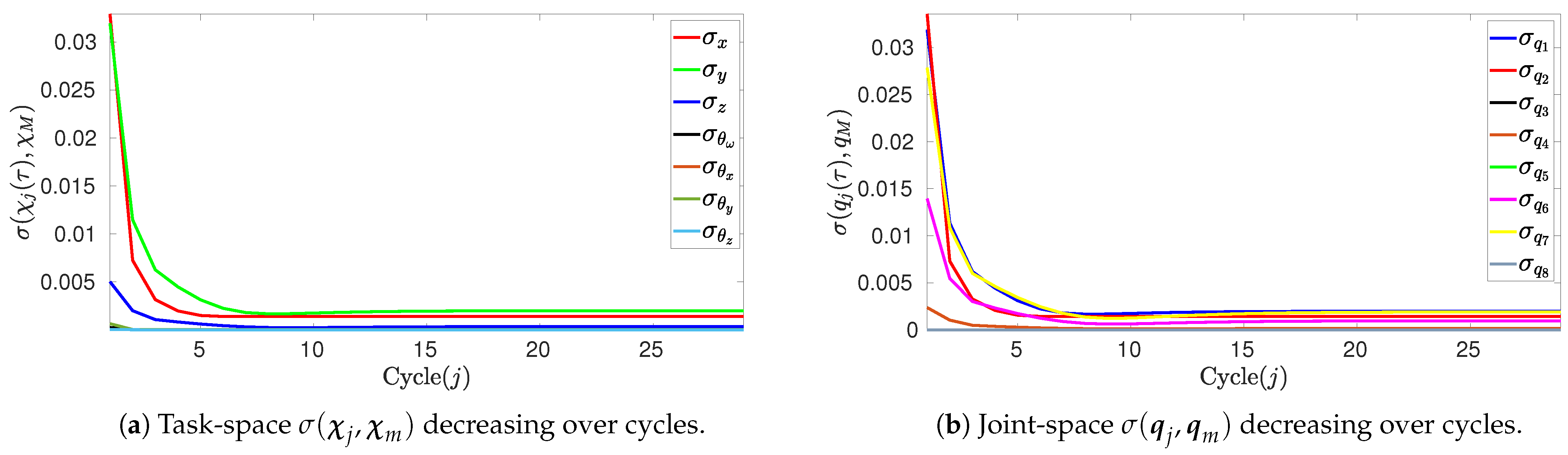
This theoretical conclusion is compatible with empirical methods to support its validity, such as the standard deviations of sampled trajectories of $(q,{\chi }^{*})$, defined as $\mathit{q}\in {\mathbb{R}}^{N\times n}$ and $\mathit{\chi }\in {\mathbb{R}}^{N,m}$, for N samples and their sample-mean ${\mathit{q}}_m$, ${\mathit{\chi }}_m$, such that, if

$$\sigma (\mathit{\chi },{\mathit{\chi }}_m)\approx 0,\sigma (\mathit{q},{\mathit{q}}_m)\approx 0,$$

(82)

it indicates repeatable and unique trajectories independent of integration path, as defined by the constructed integral manifold $({\mathit{q}}_j,{\mathit{\chi }}_j)\in \mathcal{S}$.

□

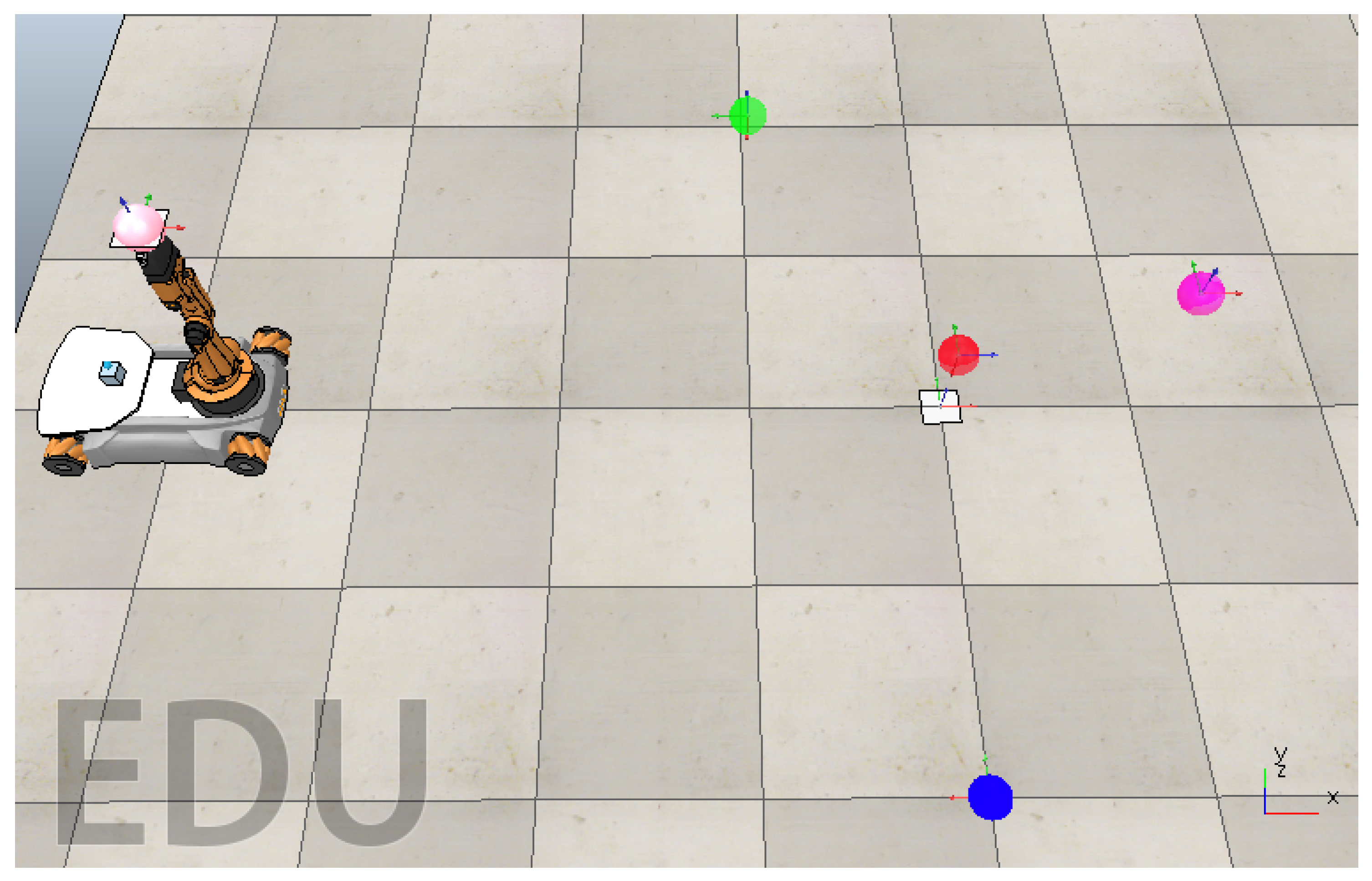
5. Simulations of an Omnidirectional Mobile Manipulator

The main objective of these simulations is to demonstrate how a robotic data-driven control system has inherent repeatability capabilities, the reason being the explicit state-independency of the data-driven estimated Jacobian, which becomes invariant to the state once the update law (67) stabilizes, leading to an integrable system that defines smooth trajectories in $q\in \mathcal{C}$, which the robot learns to follow for a given task ${\chi }_0\to {\chi }_d$. Then, for recurrent $\dot{\chi }\to {\dot{\chi }}_d$ that satisfies $\dot{q}\in {\mathcal{D}}_q$, there is the same learned trajectory $(q,\chi )\in \mathcal{S}$, which guarantees repeatability of the system.

The simulations were performed in the virtual environment CoppeliaSim Edu V4.6.0-Rev16. Jacobian estimation and closed-loop control computations were implemented using Python 3.11.5, running on an Asus laptop with 6 GB of RAM, an Intel^® Core™ i7-8550U CPU @ 1.8 GHz x 8, and Ubuntu 20.04.3 LTS (64-bit). Communication between the virtual environment and the Python framework was established via the zmq remote API functions of CoppeliaSim. By using CoppeliaSim-Python functions in an iterative loop, it is possible to read the coordinates of any object in the virtual environment and track any change in real time, similar to a motion-capture system. Additionally, it is possible to write joint coordinates to the virtual robot, triggering motion and updating the positions of all child elements, including the end-effector. Each subsequent iteration read the updated coordinates, forming a closed-loop control system involving both CoppeliaSim and Python.

5.1. Simulated Robot and Virtual Environment

The virtual workspace of CoppeliaSim is the 3D space where the robot, its end-effector, and other objects have coordinates in $\mathcal{X}$ with respect to a common frame (such as the origin). This mimics an actual industrial workstation, where ${\chi }^{*}\in \mathcal{X}$ and ${\dot{\chi }}^{*}\in \mathcal{T}\left(\mathcal{X}\right)$ are measured by real sensors, e.g., motion capture systems. There is little theoretical difference between virtual and real workspaces when it comes to the coordinate transformations involved in the frame representation of bodies. However, a virtually measured signal ${\chi }^{*}$ generally satisfies Assumption 1, such that ${\dot{\chi }}^{*}$ is well defined, while the measurements of real sensors could be subject to noise and discontinuities, greatly affecting ${\dot{\chi }}^{*}$ and (67). Fortunately, for real applications, motion capture systems have proven to be robust enough for Assumption 1 to hold [51]. Therefore, numerical differentiation of ${\chi }^{*}$ into ${\dot{\chi }}^{*}$, with methods such as Euler’s step, is well supported to provide feedback to (67), even in real field applications.

The simulated robot is a CoppeliaSim built-in model of the omnidirectional mobile manipulator Kuka-Youbot of 8-DoF. Its omnidirectional base has coordinates in $\mathrm{SE}\left(2\right)$ and can be represented by (37), assuming a perfect map between the wheels and $\mathrm{SE}\left(2\right)$. The configuration of the manipulator arm lies in ${\left({\mathbb{S}}^1\right)}^5$; thus, $\mathrm{SE}\left(2\right)\times {\left({\mathbb{S}}^1\right)}^5\triangleq \mathcal{C}$, while the task-space of the environment is ${\chi }^{*}\in \mathcal{X}$, as defined by (59); therefore, ${\chi }^{*}$ represents the coordinates of the tip of the end-effector and ${\chi }_d^{*}$ the desired coordinates attached to an object in the virtual environment.

The expression of the frame and the parameterization of ${\chi }^{*},{\chi }_d^{*}$ are based on the chosen relative transformation matrix, defined as the error that must be minimized in the identity $T_e=T_b^{t^{-1}}{T}_b^d\to I$, where $T_e\in \mathrm{SE}\left(3\right)$ and its parameterized equivalence are given by $e_p=p^{*}-p_d$ and $e_q={\theta }_q\otimes {\theta }_{qd}$, where $e={[e_p^T,e_q^T]}^T\in \mathcal{X}$. In the virtual workspace, $T_b^t=T_w^{b^{-1}}{T}_w^t$ and $T_b^d=T_w^{b^{-1}}{T}_w^d$ encode the coordinates of the end-effector’s tip frame (index t) and desired set-point frame (index d) expressed with respect to the mobile base frame (index b) by using $T_w^{b^{-1}}$. Otherwise, $T_w^t$ and $T_w^d$ are expressed in the world frame (index w), which are the default measurements obtained by the sensors that do not involve any transformation (this representation is enough to compute $T_e$ only for inertial robots with fixed bases). Note the path dependency and coupled linear and rotational coordinates in $T_e=T_b^{t^{-1}}{T}_b^d$:

$$T_e=\left[\begin{array}{cc}{R}_b^{t^T}& -R_b^{t^T}{p}_b^t\\ 0& 1\end{array}\right]\left[\begin{array}{cc}{R}_w^{b^T}{R}_w^d& R_w^{b^T}(p_w^d-p_w^b)\\ 0& 1\end{array}\right]=\left[\begin{array}{cc}{R}_b^{t^T}{R}_w^{b^T}{R}_w^d& R_b^{t^T}(R_w^{b^T}(p_w^d-p_w^b)-p_b^t)\\ 0& 1\end{array}\right].$$

(83)

Then, let $R_b^{t^T}{R}_w^{b^T}{R}_w^d=R_b^{t^T}{R}_b^d=R_t^d\triangleq e_R$ and $R_b^{t^T}(R_w^{b^T}(p_w^d-p_w^b)-p_b^t)=R_b^{t^T}(p_b^d-p_b^t)=p_t^d\triangleq e_p$. Note that the quaternion representation of $e_R$ is $e_q={\theta }_{q_b}^{t^{*}}\otimes {\theta }_{q_b}^d$; thus, $e={[e_p^T,e_q^T]}^T\in \mathcal{X}$ defines the error computed with the measured coordinates of the virtual workspace ${\chi }^{*}$, ${\chi }_d^{*}\in \mathcal{X}$.

In this simulation environment, (67)–(69) are deployed with $K_p=1$, such that $e\to 0$ provided that $ϵ\to 0$ and $\widehat{J}\to J^{*}$. The end-effector is initially at home, with a joint configuration of $q_i=0$ for all $i=1,2,\cdots ,8$, and at ${\chi }_0^{*}={[-1.8,0,0.745,1,0,0,0]}^T$ with respect to the world’s origin in the virtual environment. With the robot-at-home configuration, the initial Jacobian ${\widehat{J}}_0$ is computed with (49), only requiring the knowledge of the joint-axes alignment with respect to the world’s frame and the relative distances between them at $q=0$; also, with ${\widehat{J}}_0$, the initial ${\widehat{J}}_0^{†}$ is computed offline with (65).

The desired set-point ${\chi }_{d_i}^{*}$ was subject to changes following the time-scheduled sequence detailed in

Table 1. Scheduled desired reference changes for a cycle j. The coordinates are absolute (all with respect to the world’s inertial frame). Also, $t=(k-1)\delta t$ and ${\tau }_j=N_j\delta t$ for $k=1,2,\dots ,N_j$; thus, for $N_j$ iteration steps, ${\tau }_j=70$ s is the duration of one cycle j.

Reference	Target	Position [m]	Orientation $\left[\frac{{\mathit{\theta }}_{\mathit{q}}}{\parallel {\mathit{\theta }}_{\mathit{q}}\parallel }\right]$	Schedule [s]
${\chi }_{d_1}^{*}$	red	$(0,0,0.25)$	$[0.707,0,0.707,0]$	$t\le 10$
${\chi }_{d_2}^{*}$	blue	$(0,-1,0)$	$[0,0,-1,0]$	$10<t\le 20$
${\chi }_{d_3}^{*}$	purple	$(0.5,0,0.5)$	$[1,0,0,0]$	$20<t\le 30$
${\chi }_{d_4}^{*}$	red	$(0,0,0.25)$	$[0.707,0,0.707,0]$	$30<t\le 40$
${\chi }_{d_5}^{*}$	green	$(-0.5,0.7,0.35)$	$[0.5,-0.5,0.5,0.5]$	$40<t\le 50$
${\chi }_{d_6}^{*}$	red	$(0,0,0.25)$	$[0.707,0,0.707,0]$	$50<t\le 60$
${\chi }_{d_7}^{*}$	beige (home)	$(-1.8,0,0.745)$	$[1,0,0,0]$	$60<t\le 70$

. Notice that ${\chi }_0^{*}={\chi }_{d_7}^{*}$, which means that the initial home configuration of ${\chi }_0^{*}$ is also a recurrent last reference before the end of a cycle; that is, the robot is tasked to return to home configuration so that a new cycle begins. The virtual environment with the robot’s home position and the location of the objects is illustrated in Figure 1. The simulation for this experiment is presented in a video available at https://drive.google.com/file/d/1Aabi_boDPGRXCPyOrcSJnMKuo0H1nBL-/view?usp=sharing (accessed on 20 February 2025).

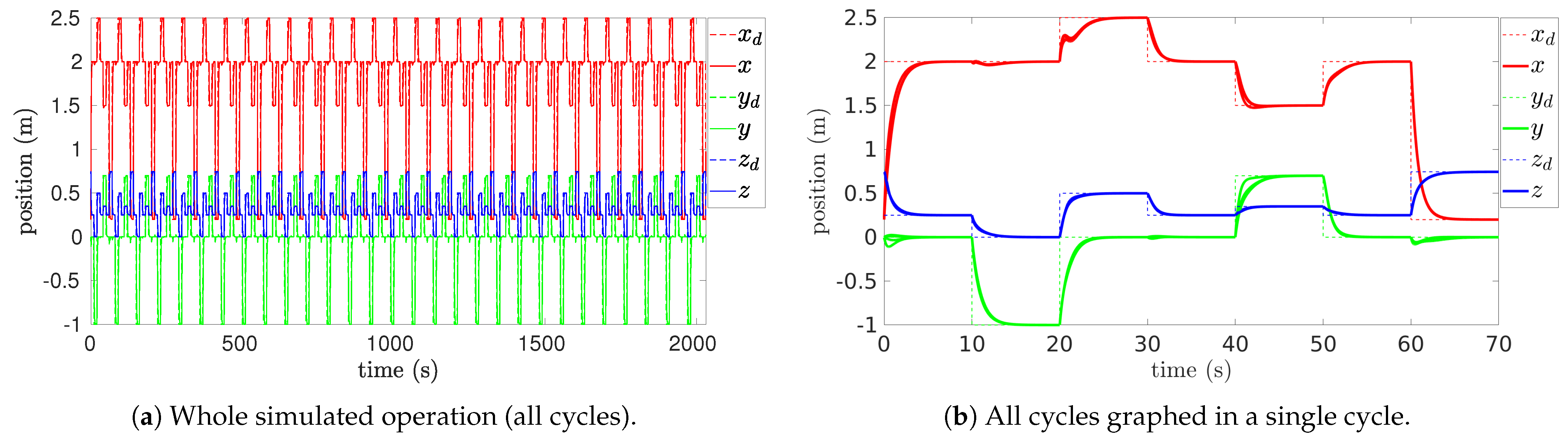
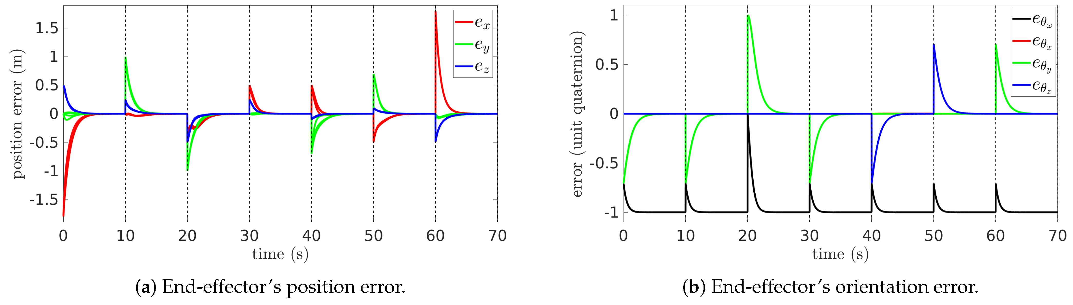
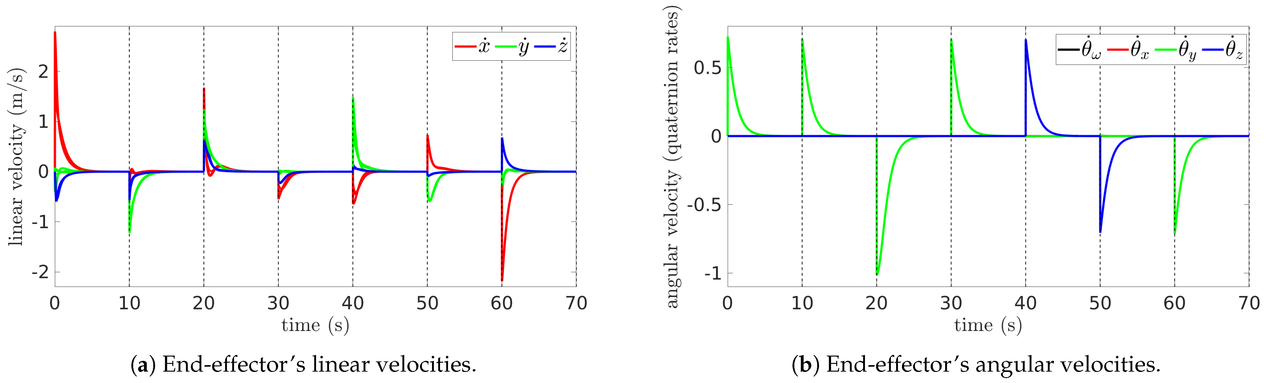
5.2. Simulation Results

Note that the values of ${\chi }_d^{*}=[p_d^{*},{\theta }_{qd}^{*}]$, changing over the time schedule of Table 1, are absolute as they are measured with respect to the world’s frame (origin). However, note that the robot $p_d^{*}\left(0\right)$ is not at the origin. Therefore, with (83), the absolute commands given to $p_d^{*}$ change into relative commands with respect to the current manipulator’s mobile base such that an error can be computed. Note that, since ${\theta }_{qd}^{*}\left(0\right)$ is aligned with the world’s frame orientation, no distinction between absolute and relative commands is needed to compute the orientation error.

In Figure 2 and Figure 3, the commands ${\chi }_{d_i}^{*}$ (dashed lines) change in a discrete discontinuous manner (every 10 s) from ${\chi }_{d_1}^{*}\to {\chi }_{d_2}^{*}\to \cdots \to {\chi }_{d_7}^{*}$. Thus, ${\chi }_{d_i}^{*}$ is constant between the dashed vertical lines, where ${\chi }^{*}$ (continuous lines) converges to ${\chi }_{d_i}^{*}$. Thus, a cycle ${\chi }_{d_1}^{*}\to \cdots \to {\chi }_{d_7}^{*}$ lasts a total of 70 s. For a repetitive execution of 29 cycles, the total duration of the whole simulation is 2030 s, settled to 2000 s or 33.33 min.

Figure 2 shows the position commands $p_d^{*}$, initially specified by the absolute coordinates of the bodies in Figure 1, then transformed by (83). The dashed lines correspond to the relative desired coordinates ($x_d$, $y_d$, $z_d$); the continuous lines correspond to the relative end-effector coordinates (x, y, z). Figure 2a shows the position commands over the entire simulation (2000 s) and the end-effector’s position evolution; since commands are repetitive over cycles, it is possible to overlay the cycles into the duration of a single cycle (70 s), as in Figure 2b, where the end-effector’s position evolution (continuous lines) shows near-perfect alignment, indicating highly consistent performance with minimal deviation between cycles.

Figure 3 presents the desired orientation commands (${\theta }_{\omega d}$, ${\theta }_{xd}$, ${\theta }_{yd}$, ${\theta }_{zd}$) as dashed lines and end-effector current orientation (${\theta }_{\omega }$, ${\theta }_x$, ${\theta }_y$, ${\theta }_z$) as continuous lines. The orientations are represented with unit quaternions and without a required distinction of absolute and relative values. Figure 3a shows the orientation commands throughout the simulation (2000 s), whereas Figure 3b shows the same commands overlaid along the duration of a cycle (70 s), underscoring the alignment of the actual orientation of the end-effector between cycles, which demonstrates a consistent and repeatable performance of the robotic manipulator during cyclic tasks.

Note that the behavior of ${\chi }^{*}$ to track ${\chi }_{d_1}\to {\chi }_{d_7}$ consistently across cycles suggests (73), e.g., the formation of integrable velocity maps ${\dot{\chi }}_{d_i}^{*}\to \dot{q}$, which define subspaces ${\mathcal{D}}_{q_i}$ that uniquely lead ${\chi }^{*}\in \mathcal{S}$ to converge into ${\chi }_{d_i}^{*}$ in any cycle.

The graphs in Figure 4 illustrate the evolution of the end-effector’s position and orientation errors during the execution of repetitive cyclic tasks, consolidating the position error signals ($e_x$, $e_y$, and $e_z$) in Figure 4a and the orientation error signals ($e_{{\theta }_{\omega }}$, $e_{{\theta }_x}$, $e_{{\theta }_y}$, and $e_{{\theta }_z}$) in Figure 4b from all cycles into a single cycle. The error converges to near-zero values after each change in reference ${\chi }_{d_i}^{*}$ (dotted vertical lines), highlighting the effectiveness of the proposed data-driven controller in ensuring accurate positioning. Furthermore, the near-identical overlap of the error profiles underscores the system’s ability to maintain repeatability across numerous iterations.

Figure 5 illustrates the velocities of the end-effector overlayed in a single cycle to contrast its evolution across cycles. The linear velocities ($\dot{x}$, $\dot{y}$, $\dot{z}$) of Figure 5a are a direct differentiation of the relative positions (with respect to the mobile base): ${\dot{p}}_k^{*}={\displaystyle \frac{p_k^{*}-p_{k-1}^{*}}{\delta t}}$, which becomes the feedback for (67). Figure 5b shows the angular velocities (${\dot{\theta }}_{\omega }$, ${\dot{\theta }}_x$, ${\dot{\theta }}_y$, ${\dot{\theta }}_z$) that result from ${\dot{\widehat{\theta }}}_q={\widehat{J}}_{\theta }\dot{q}$ since $\dot{q}$ represents the joint velocities computed with (69), and then ${\dot{\widehat{\theta }}}_q\to {\dot{\theta }}_q^{*}$ as ${\widehat{J}}_{\theta }\to J_{\theta }^{*}$. Therefore, if $ϵ\to 0$, then ${\dot{\theta }}_q$ becomes equivalent to the angular velocity measurements needed as feedback for (67).

Figure 6 presents the estimation errors of (67), with Figure 6a demonstrating periodic consistent behavior of $ϵ$ due to uniform changes in reference across cycles of the form ${\chi }_{d_i}^{*}\to {\chi }_{d_i}^{*}+\mathrm{\Delta }{\chi }_d^{*}={\chi }_{d_{i+1}}^{*}$. Figure 6b shows the evolution of $ϵ$ of all overlaid cycles, which align almost perfectly. Note how $ϵ$ increases at the beginning of a change in reference (dotted vertical lines) in the same direction of $\mathrm{\Delta }{\chi }_d^{*}$ and a magnitude $\parallel ϵ\parallel \propto {\displaystyle \frac{1}{\gamma }}\parallel \mathrm{\Delta }{\chi }_d^{*}\parallel$. This magnitude bound keeps $\parallel {ϵ}_k\parallel <\parallel e_k\parallel$$\forall k\ge 0$, with $ϵ$ decaying faster than e. Also, note that $({ϵ}_x,{ϵ}_y,{ϵ}_z)$ are the coordinates that increase significantly during $\parallel \mathrm{\Delta }{\chi }_d^{*}\parallel >0$, while $({ϵ}_{{\theta }_{\omega }},{ϵ}_{{\theta }_x},{ϵ}_{{\theta }_y},{ϵ}_{{\theta }_z})$ remain unchanged since $k\ge 0$. One reason is that $\max (\parallel \mathrm{\Delta }{\theta }_q^{*}\parallel )=1$ due to the unit quaternion constraint, while $\parallel \mathrm{\Delta }{p}^{*}\parallel$ is unbounded and can grow as much as feasible for the robot workspace. The other reason is the range of ${\widehat{J}}_k$$\forall k\ge 0$, which, from its initial guess ${\widehat{J}}_0$, is able to generate velocities in the directions of ${\theta }_y$ and ${\theta }_z$, which are sufficient for tasks that require pointing the end-effector towards an objective in the workspace.

At this stage of the analysis, the behaviors of ${\chi }^{*}$ in Figure 2 and Figure 3, of e in Figure 4, and particularly of $ϵ$ in Figure 6 suggest that (73) is generated before $e\to 0$.

Figure 7 illustrates the joint velocities that result from the control law (69), which drives ${\dot{\chi }}^{*}$ through the robot mechanism $J^{*}:\dot{q}\to {\dot{\chi }}^{*}$, which also becomes a feedback signal for (67). Figure 7a shows the periodic behavior of the joint velocities, which is confirmed by the negligible deviations across cycles in Figure 7b. The periodic behavior of $\widehat{J}:\dot{q}\to {\dot{\chi }}^{*}$ is consistent with Figure 2, Figure 3 and Figure 4. Thus, if $\dot{q}$ uniquely generates ${\dot{\chi }}^{*}$ across cycles, then ${\dot{\chi }}^{*}-\widehat{J}\dot{q}\in {\mathcal{D}}_q$ is an integrable constraint that leads to a subset of $(q,{\chi }^{*})\in \mathcal{S}$ that uniquely defines ${\chi }_{d_i}$ and its changes through ${\chi }_{d_1}\to \dots \to {\chi }_{d_7}$, which explains the repetitiveness.

Figure 8 presents the joint positions ($q_1$ to $q_8$) of the 8-DoF KUKA YouBot during cyclic tasks. Figure 8a shows the evolution of the joint positions over the entire simulation period, demonstrating consistent periodic behavior for all joints. The trajectories reveal minor variations in amplitude and phase across the joints, indicating negligible differences in how q relates to the end-effector’s current state ${\chi }^{*}$ across cycles. Figure 8b overlays all cycles to highlight how the trajectories align almost perfectly with negligible deviations across cycles. This alignment suggests that integrating $\dot{q}\in {\mathcal{D}}_q$, with ${\mathcal{D}}_q={\bigcup }_{i=1}^7{\mathcal{D}}_{q_i}$ generates a trajectory $(q,{\chi }^{*})\in \mathcal{S}$ that uniquely goes through the sequence ${\chi }_{d_1}\to {\chi }_{d_i}\to {\chi }_{d_7}$ in every cycle (Table 1).

The results shown in Figure 4 and Figure 8 qualitatively suggest repeatability in the task-space and joint-space when observing the overlaid values aligned across cycles. However, the foundation of repeatability in this work can also be proven quantitatively with statistical validation metrics, such as the standard deviation of the end-effector’s trajectory ${\chi }_{\mathit{j}}\left({\tau }_j\right)=[{\mathit{p}}_j\left({\tau }_j\right),{\mathit{\theta }}_j\left({\tau }_j\right)]$ generated along a cycle j and sampled at each $t=k{\delta }_t$ for $k=1,2,\dots ,N_j$, where ${\delta }_t=0.01$ and ${\tau }_j=N_j{\delta }_t$. Thus, ${\mathit{\chi }}_j\left({\tau }_j\right)\in {\mathbb{R}}^{N_j\times 7}$ is sampled for every cycle $j=1,2,\dots N_c$ such that a trajectory-sample-mean can be computed as ${\mathit{\chi }}_m={\displaystyle \frac{1}{N_c}}{\sum }_{j=1}^{N_c}{\mathit{\chi }}_j\left({\tau }_j\right)$, where the standard deviation is given by

$$\sigma ({\mathit{\chi }}_j,{\mathit{\chi }}_m)=\sqrt{{\displaystyle \frac{1}{N_c-1}}\sum _{i=1}^{N_c}{({\mathit{\chi }}_j-{\mathit{\chi }}_m)}^2}.$$

(84)

Now, let ${\mathit{q}}_j\left({\mathsf{\tau }}_j\right)\in {\mathbb{R}}^{N_j\times 8}$ be the joint-space trajectory generated along a cycle j and sampled similarly to ${\mathit{\chi }}_j\left({\tau }_j\right)$. The joint-space trajectory-sample-mean is then ${\mathit{q}}_m={\displaystyle \frac{1}{N_c}}{\sum }_{j=1}^{N_c}{\mathit{q}}_j\left({\tau }_j\right)$, and the standard deviation $\sigma ({\mathit{q}}_j,{\mathit{q}}_m)$ is computed similarly to (84).

It can be seen in Figure 9a that maximum values of $\sigma ({\mathit{\chi }}_j,{\mathit{\chi }}_m)$ occur in the first cycle $j=1$, mainly ${\sigma }_x=0.033$ m and ${\sigma }_y=0.031$ m, corresponding to the coordinates along which the end-effector moves the most (it belongs to a mobile manipulator on the $x,y$-plane). Meanwhile, ${\sigma }_z$ has less variability as the vertical motion of the end-effector is limited by the reach of its manipulator arm. Also, $({\sigma }_{{\theta }_{\omega }},{\sigma }_{{\theta }_x},{\sigma }_{{\theta }_y},{\sigma }_{{\theta }_z})$ show negligible deviations from the mean. Then, from cycle $j>6$ up to $j=N_c=29$, all the coordinates in $\sigma ({\mathit{\chi }}_j,{\mathit{\chi }}_m)$ converge to minimal values, with ${\sigma }_x\approx {\sigma }_y\approx 0.001$ m, whereas ${\sigma }_z\approx 3.0\times {10}^{-4}$ and ${\sigma }_{{\theta }_{\omega }}\approx {\sigma }_{{\theta }_x}\approx {\sigma }_{{\theta }_y}\approx {\sigma }_{{\theta }_z}\approx 1.4\times {10}^{-6}$. The reason why the standard deviation is larger in cycle $j=1$ is that the end-effector begins the cycle from a steady state and an initial Jacobian estimate; then, when $j>1$, the robot begins the cycle anew with a better estimation of the Jacobian, which is a process that improves over cycles. Note that the overall small values of the standard deviation are consistent with the results observed in Figure 2 and Figure 3. Figure 9b shows the standard deviation of each coordinate of ${\mathit{q}}_j={[q_1,q_2,\dots q_8]}_j^T$ in each cycle $j=1,2\dots ,29$. The maximum values of $\sigma ({\mathit{q}}_j,{\mathit{q}}_m)$ also occur at $j=1$, with ${\sigma }_{q_1}=0.033$ m, ${\sigma }_{q_2}=0.031$, and ${\sigma }_{q_7}=0.027$ radians. Then, from cycle $j>6$ up to $j=N_c=29$, all the coordinates in $\sigma ({\mathit{q}}_j,{\mathit{q}}_m)$ converge to minimal values, with ${\sigma }_{q_1}\approx {\sigma }_{q_2}\approx 0.001$ m and ${\sigma }_{q_7}\approx 0.001$ radians as maximum values. Note that the overall small values of the standard deviations are consistent with the results observed in Figure 8, which validates the theoretical foundation of Theorem 1; that is, if $\sigma ({\mathit{q}}_j,{\mathit{q}}_m)\approx \sigma ({\mathit{\chi }}_j,{\mathit{\chi }}_m)\approx 0$, then $({\mathit{q}}_j,{\mathit{\chi }}_j)\in \mathcal{S}$.

The evolution of the position-partition of the estimated Jacobian, computed with (67), is depicted in Figure 10, where each graph corresponds to a row of $\widehat{J}$. Each row relates an axis of the position coordinate $(x,y,z)$ with all joint coordinates $q_i$, describing how much influence the joint-space has on such a position coordinate when it comes to mapping velocities. Note how the Jacobian changes only at the beginning of reference changes $\mathrm{\Delta }{\chi }_{d_i}$ (dotted vertical lines), then settles again into steady values. The regions between the dotted vertical lines describe the creation of ${\mathcal{D}}_{q_i}$, as described by (72), and the regions where the values of $\widehat{J}$ are steady contribute to (73), where (6) and (17) are satisfied.

When contrasting the values that the rows of $\widehat{J}$ take along the duration of a cycle, for each cycle, it is possible to observe different adaptation behaviors, specifically during the initial cycles (dotted lines before cycle 6, which agree with the results observed in Figure 9). The difference in the adaptation behavior comes from the robot engaging the first cycle in a steady state (at the beginning of the simulation), with an initial Jacobian estimate ${\widehat{J}}_0$. Therefore, once the robot ends the first cycle, it begins the second cycle by performing the same actions but with a renewed ${\widehat{J}}_k$; thus, each time, the adaptation of $\widehat{J}$ changes slightly in every cycle until reaching a consensus of how $\widehat{J}$ should adapt itself to perform the different routines of the cycle. At a terminal number of cycles, the end-resulting behavior of $\widehat{J}$ could be seen as if it had never had a steady state.

The results of Figure 11 are quite interesting as the Jacobian orientations, parameterized with unit quaternions, remain constant all along. This means that, from the initial guess definition ${\widehat{J}}_0$ to the end, the range-space was enough to move in the coordinates required by every cycle routine, certainly enough to not require any update at all. To explain this, consider that the end-effector’s orientation is initially aligned to the mobile base’s and world frame’s orientations; thus, there is no distinction between relative or absolute coordinates when computing $e_{\theta }$. In addition, ${\widehat{J}}_0$ is defined considering the robot in its home position with $q_i=0$$\forall i=1\dots 8$. It happens that, from its home position, the end-effector can rotate about the y-axis (${\theta }_y$) involving $\left\{q_5,q_6,q_7\right\}$ (the only non-zero coordinates in Figure 11b) and about the z-axis (${\theta }_z$) involving $\left\{q_3,q_4\right\}$ (the only non-zero coordinates in Figure 11c). However, it does not have a direct way to rotate about the x-axis (${\theta }_x$) since no $q_i$-axes are originally aligned to the world frame’s x-axis, which also explains why Figure 11a shows that ${\widehat{J}}_{{\theta }_x}$ contains all zero values as it cannot map angular velocities about the x-axis. Rotation about the x-axis is possible only when the end-effector is at ±90° about the y-axis, allowing the end-effector to rotate about its own axis of motion with $q_8$. Now, consider that, with ${\theta }_y$ and ${\theta }_z$, the end-effector can be oriented to face any direction in the 3D space (except that it cannot rotate on its own axis); this remains true regardless of current values of $q_i\ne 0$; therefore, ${\theta }_y$ and ${\theta }_z$ can be interpreted as defined globally, with fixed $y,z$-axes, such that ${\widehat{J}}_{{\theta }_y}$ and ${\widehat{J}}_{{\theta }_z}$ remain constant. Since no task ${\chi }_{d_i}^{*}$ requires the end-effector to rotate on its own axis of motion, then ${\theta }_x$ is an unnecessary DoF, and the corresponding row ${\widehat{J}}_{{\theta }_x}$ remains as initially defined (a row of zeros).

Figure 12 denotes the result of computing (12), which is equivalent to (19), except that condition $d\left(du\right)=0$ is being evaluated. However, the columns of $\widehat{J}$, computed by (67), cannot be treated as basis twists as they directly map $\widehat{J}:\dot{q}\to {\dot{\theta }}_q$. Thus, the Lie brackets cannot be computed numerically with cross-products; rather, the partial derivatives were approximated with finite differentiations. Note that condition $d\left(du\right)=0$ is satisfied when $\dot{e}-\widehat{J}\dot{q}=0$, which coincides with the times of the vertical dotted lines, that is, when the Jacobian becomes a constant optimal basis (Figure 10 and Figure 11).

6. Conclusions

This study has demonstrated that the implementation of a data-driven control system utilizing an estimated Jacobian significantly enhances the repeatability of robotic movements. The findings indicate that the estimated Jacobian becomes invariant to the state once the update law stabilizes, leading to an integrable system that defines smooth trajectories. This integrability is crucial for achieving consistent motion across cyclic tasks, thereby ensuring repeatability in the robot’s performance. The results confirm that the proposed approach not only establishes the necessary conditions for repeatability but also reduces the computational costs compared to traditional analytical model-based methods. Overall, the integration of the estimated Jacobian provides a robust framework for improving the repeatability of redundant robots in various applications.

Furthermore, the computational cost online of the proposed method was found to be 95% lower (for $n=8$ and $m=6$) than the conventional analytical model-based control strategies due to the estimation of the inverse of the Jacobian matrix.

The approach proposed involves point-to-point regulation control in the task-space, which only minimizes the control error exponentially, with no explicit possibility of accelerating the convergence time at will. Increasing the proportional control gain leads to faster convergence to the reference points; on the other hand, the speed of convergence of the control error is limited by the convergence of the estimator error to achieve an adequate velocity map from the estimated Jacobian matrix. However, a longer convergence time must be guaranteed for the control error than for the estimation error. Therefore, there is a minimum time bounded by the adaptation time of the updated law estimation algorithm, which depends on the characteristics of the robot, the uncertainties, and the tuning parameters of the estimation algorithm.

The data-driven model approach demonstrated high accuracy and repeatability in controlling the end-effector pose in the cycling task. Its performance is influenced by the quality of the input data; however, this dependency can be mitigated by employing robust sensing strategies and filtering techniques. Future work will explore strategies to enhance generalization in scenarios with limited and noisy feedback, and to establish the minimal convergence time that is feasible for a data-driven approach, when performing tasks with predefined time convergence. Moreover, the incorporation of secondary tasks for data-driven approaches in a hierarchical scheme would further exploit the potential of data-driven approaches.

References

1. Cañas, H.; Mula, J.; Díaz-Madroñero, M.; Campuzano-Bolarín, F. Implementing industry 4.0 principles. Comput. Ind. Eng. 2021, 158, 107379. [Google Scholar] [CrossRef]
2. Ribeiro, J.; Lima, R.; Eckhardt, T.; Paiva, S. Robotic process automation and artificial intelligence in industry 4.0—A literature review. Procedia Comput. Sci. 2021, 181, 51–58. [Google Scholar]
3. Axmann, B.; Harmoko, H. Robotic process automation: An overview and comparison to other technology in industry 4.0. In Proceedings of the 2020 10th International Conference on Advanced Computer Information Technologies (ACIT), Deggendorf, Germany, 16–18 September 2020; pp. 559–562. [Google Scholar]
4. Urrutia, P.; Guamán-Molina, J.; Peñaloza, A.; Salazar, F.; Madroñero, D.G.; Jácome, J.A. Control System for the Teleoperation of Kuka Youbot Robot via Wireless Communication and the Use of Embedded Cards. In Proceedings of the International Conference on Computer Science, Electronics and Industrial Engineering (CSEI), Ambato, Ecuador, 6–10 November 2023; Springer: Cham, Switzerland, 2023; pp. 615–628. [Google Scholar]
5. Pająk, G.; Pająk, I. Trajectory Planning for Mobile Manipulators with Control Constraints. Pomiary Autom. Robot. 2023, 27, 21–30. [Google Scholar]
6. Hernandez-Barragan, J.; Villaseñor, C.; Lopez-Franco, C.; Arana-Daniel, N.; Gomez-Avila, J. Image based visual servoing with kinematic singularity avoidance for mobile manipulator. PeerJ Comput. Sci. 2024, 10, e2559. [Google Scholar] [CrossRef]
7. Zhang, Y.; Jia, Y. Motion planning of redundant dual-arm robots with multicriterion optimization. IEEE Syst. J. 2023, 17, 4189–4199. [Google Scholar]
8. Zheng, L.; Zhang, Z. Time-varying quadratic-programming-based error redefinition neural network control and its application to mobile redundant manipulators. IEEE Trans. Autom. Control 2021, 67, 6151–6158. [Google Scholar]
9. Hou, Z.; Chi, R.; Gao, H. An overview of dynamic-linearization-based data-driven control and applications. IEEE Trans. Ind. Electron. 2016, 64, 4076–4090. [Google Scholar]
10. Treesatayapun, C. Data-driven fault-tolerant control with fuzzy-rules equivalent model for a class of unknown discrete-time MIMO systems and complex coupling. J. Comput. Sci. 2022, 63, 101827. [Google Scholar]
11. Treesatayapun, C. Fuzzy rules emulated discrete-time controller based on plant’s input–output association. J. Control Autom. Electr. Syst. 2019, 30, 902–910. [Google Scholar]
12. Campos-Torres, I.; Gómez, J.; Baltazar, A. Data-Driven Adaptive Force Control for a Novel Soft-Robot Based on Ultrasonic Atomization. In Proceedings of the Advances in Computational Intelligence: 21st Mexican International Conference on Artificial Intelligence, MICAI 2022, Monterrey, Mexico, 24–29 October 2022; Proceedings, Part II. Springer: Berlin/Heidelberg, Germany, 2022; pp. 279–290. [Google Scholar]
13. Gao, S.; Zhao, D.; Yan, X.; Spurgeon, S.K. Model-Free Adaptive State Feedback Control for a Class of Nonlinear Systems. IEEE Trans. Autom. Sci. Eng. 2023, 21, 1824–1836. [Google Scholar]
14. Liu, T.; Hou, Z. Model-Free Adaptive Containment Control for Unknown Multi-Input Multi-Output Nonlinear MASs with Output Saturation. IEEE Trans. Circuits Syst. Regul. Pap. 2023, 70, 2156–2166. [Google Scholar] [CrossRef]
15. Hou, Z.; Jin, S. Model Free Adaptive Control: Theory and Applications; CRC Press: Boca Raton, FL, USA, 2013. [Google Scholar]
16. Esmaeili, B.; Baradarannia, M.; Salim, M.; Farzamnia, A. Data-driven MIMO discrete-time predictive model-free adaptive integral terminal sliding mode controller design for robotic manipulators driven by pneumatic artificial muscles. In Proceedings of the 2019 6th International Conference on Control, Instrumentation and Automation (ICCIA), Sanandaj, Kurdistan, 30–31 October 2019; pp. 1–8. [Google Scholar]
17. Tutsoy, O.; Barkana, D.E.; Tugal, H. Design of a completely model free adaptive control in the presence of parametric, non-parametric uncertainties and random control signal delay. ISA Trans. 2018, 76, 67–77. [Google Scholar] [CrossRef]
18. Gómez, J.; Treesatayapun, C.; Morales, A. Multi-Inputs and Multi-Outputs equivalent model based on data driven controller for a robotic system. IFAC-PapersOnLine 2020, 53, 9784–9789. [Google Scholar] [CrossRef]
19. Gómez, J.; Treesatayapun, C.; Morales, A. Data-driven identification and control based on optic tracking feedback for robotic systems. Int. J. Adv. Manuf. Technol. 2021, 113, 1485–1503. [Google Scholar] [CrossRef]
20. Yang, C.; Jiang, Y.; Na, J.; Li, Z.; Cheng, L.; Su, C.Y. Finite-Time Convergence Adaptive Fuzzy Control for Dual-Arm Robot with Unknown Kinematics and Dynamics. IEEE Trans. Fuzzy Syst. 2019, 27, 574–588. [Google Scholar] [CrossRef]
21. Li, M.; Kang, R.; Branson, D.T.; Dai, J.S. Model-free control for continuum robots based on an adaptive Kalman filter. IEEE/ASME Trans. Mechatron. 2017, 23, 286–297. [Google Scholar] [CrossRef]
22. Goméz-Casas, J.; Toro-Arcila, C.A.; Rodríguez-Rosales, N.A.; Obregón-Flores, J.; Ortíz-Ramos, D.E.; Martínez-Villafañe, J.F.; Gómez-Casas, O. Data-Driven Kinematic Model for the End-Effector Pose Control of a Manipulator Robot. Processes 2024, 12, 2831. [Google Scholar] [CrossRef]
23. Brake, M.; Schwingshackl, C.; Reuß, P. Observations of variability and repeatability in jointed structures. Mech. Syst. Signal Process. 2019, 129, 282–307. [Google Scholar] [CrossRef]
24. Yang, C.; Liang, M.; Xingbao, L.; Yangqiu, X.; Teng, Q.; Han, L. Uncertainty evaluation of measurement of orientation repeatability for industrial robots. Ind. Robot Int. J. Robot. Res. Appl. 2020. ahead-of-print. [Google Scholar]
25. Yang, C.; Liu, X.; Xiaobin, Y.; Mi, L.; Wang, J.; Xia, Y.; Yu, H.; Heng, C. Uncertainty analysis and evaluation of measurement of the positioning repeatability for industrial robots. Ind. Robot 2018, 45, 492–504. [Google Scholar]
26. Slotine, J.J. Robustness issues in robot control. In Proceedings of the 1985 IEEE International Conference on Robotics and Automation, St. Louis, MO, USA, 19–23 May 1985; Volume 2, pp. 656–661. [Google Scholar]
27. Zhang, F.; Zhang, X.; Li, Q.; Zhang, H. Universal nonlinear disturbance observer for robotic manipulators. Int. J. Adv. Robot. Syst. 2023, 20, 17298806231167669. [Google Scholar]
28. Yoo, B.K.; Ham, W.C. Adaptive control of robot manipulator using fuzzy compensator. IEEE Trans. Fuzzy Syst. 2000, 8, 186–199. [Google Scholar]
29. Neila, M.B.R.; Tarak, D. Adaptive terminal sliding mode control for rigid robotic manipulators. Int. J. Autom. Comput. 2011, 8, 215–220. [Google Scholar]
30. Kolhe, J.P.; Shaheed, M.; Chandar, T.; Talole, S. Robust control of robot manipulators based on uncertainty and disturbance estimation. Int. J. Robust Nonlinear Control 2013, 23, 104–122. [Google Scholar]
31. Yin, X.; Pan, L. Enhancing trajectory tracking accuracy for industrial robot with robust adaptive control. Robot. Comput.-Integr. Manuf. 2018, 51, 97–102. [Google Scholar]
32. Obregón-Flores, J.; Arechavaleta, G.; Becerra, H.M.; Morales-Díaz, A. Predefined-time robust hierarchical inverse dynamics on torque-controlled redundant manipulators. IEEE Trans. Robot. 2021, 37, 962–978. [Google Scholar]
33. Klein, C.A.; Huang, C.H. Review of pseudoinverse control for use with kinematically redundant manipulators. IEEE Trans. Syst. Man Cybern. 1983, SMC-13, 245–250. [Google Scholar]
34. Shamir, T.; Yomdin, Y. Repeatability of redundant manipulators: Mathematical solution of the problem. IEEE Trans. Autom. Control 1988, 33, 1004–1009. [Google Scholar]
35. Roberts, R.; Maciejewski, A. Repeatable generalized inverse control strategies for kinematically redundant manipulators. IEEE Trans. Autom. Control 1993, 38, 689–699. [Google Scholar]
36. De Luca, A.; Lanari, L.; Oriolo, G. Control of redundant robots on cyclic trajectories. In Proceedings of the 1992 IEEE International Conference on Robotics and Automation, Nice, France, 12–14 May 1992; Volume 1, pp. 500–506. [Google Scholar]
37. Michellod, Y.; Mullhaupt, P.; Gillet, D. On Achieving Periodic Joint Motion for Redundant Robots. IFAC Proc. Vol. 2008, 41, 4355–4360. [Google Scholar]
38. Schaufler, R.; Fedrowitz, C.; Kammuller, R. A simplified criterion for repeatability and its application in constraint path planning problems. In Proceedings of the 2000 IEEE/RSJ International Conference on Intelligent Robots and Systems (IROS 2000) (Cat. No.00CH37113), Takamatsu, Japan, 31 October–5 November 2000; Volume 3, pp. 2345–2350. [Google Scholar]
39. Mukherjee, R. Design of holonomic loops for repeatability in redundant manipulators. In Proceedings of the 1995 IEEE International Conference on Robotics and Automation, Piscataway, NJ, USA, 21–27 May 1995; Volume 3, pp. 2785–2790. [Google Scholar]
40. Zhang, Y.; Zhang, Z. Repetitive Motion Planning and Control of Redundant Robot Manipulators; Springer Publishing Company: Berlin/Heidelberg, Germany, 2013. [Google Scholar]
41. Cefalo, M.; Oriolo, G.; Vendittelli, M. Planning safe cyclic motions under repetitive task constraints. In Proceedings of the 2013 IEEE International Conference on Robotics and Automation, Karlsruhe, Germany, 6–10 May 2013; pp. 3807–3812. [Google Scholar]
42. Oriolo, G.; Cefalo, M.; Vendittelli, M. Repeatable Motion Planning for Redundant Robots over Cyclic Tasks. IEEE Trans. Robot. 2017, 33, 1170–1183. [Google Scholar]
43. Cang, N.; Guo, D.; Zhang, W.; Shen, L.; Li, W. A new discrete-time repetitive motion planning scheme based on pseudoinverse formulation for redundant robot manipulators with joint constrains. Robot. Auton. Syst. 2024, 176, 104689. [Google Scholar]
44. Islam, R.U.; Iqbal, J.; Manzoor, S.; Khalid, A.; Khan, S. An autonomous image-guided robotic system simulating industrial applications. In Proceedings of the 2012 7th International Conference on System of Systems Engineering (SoSE), Genoa, Italy, 16–19 July 2012; pp. 344–349. [Google Scholar]
45. Yu, Q.; Wang, G.; Hua, X.; Zhang, S.; Song, L.; Zhang, J.; Chen, K. Base position optimization for mobile painting robot manipulators with multiple constraints. Robot. Comput.-Integr. Manuf. 2018, 54, 56–64. [Google Scholar]
46. Gracia, L.; Solanes, J.E.; Munoz-Benavent, P.; Miro, J.V.; Perez-Vidal, C.; Tornero, J. Adaptive sliding mode control for robotic surface treatment using force feedback. Mechatronics 2018, 52, 102–118. [Google Scholar]
47. Saxena, A.; Kumar, J.; Sharma, K.; Roy, D. Controlling of Manipulator for Performing Advance Metal Welding. In Recent Innovations in Mechanical Engineering: Select Proceedings of ICRITDME 2020; Springer: Berlin/Heidelberg, Germany, 2022; pp. 41–48. [Google Scholar]
48. Lynch, K.M.; Park, F.C. Modern Robotics: Mechanics, Planning, and Control, 1st ed.; Cambridge University Press: New York, NY, USA, 2017. [Google Scholar]
49. Spong, M.; Hutchinson, S.; Vidyasagar, M. Robot Modeling and Control; Wiley select coursepack; Wiley: Hoboken, NJ, USA, 2005. [Google Scholar]
50. Hou, Z.; Jin, S. Data-driven model-free adaptive control for a class of MIMO nonlinear discrete-time systems. IEEE Trans. Neural Netw. 2011, 22, 2173–2188. [Google Scholar]
51. Gómez, J.; Morales, A.; Treesatayapun, C.; Muñiz, R. Data-driven-modelling and Control for a Class of Discrete-Time Robotic System Using an Adaptive Tuning for Pseudo Jacobian Matrix Algorithm. In Proceedings of the Advances in Computational Intelligence: 21st Mexican International Conference on Artificial Intelligence, MICAI 2022, Monterrey, Mexico, 24–29 October 2022; Proceedings, Part II. Springer: Berlin/Heidelberg, Germany, 2022; pp. 291–302. [Google Scholar]
Figure 1. CoppeliaSim’s virtual workspace (top view): the omnidirectional mobile manipulator is at home position, and colored objects each have a different workspace configuration χ d i * X .
Processes 13 00953 g001
Figure 2. Commands of relative positions for end-effector, expressed with respect to the omnidirectional base.
Processes 13 00953 g002
Figure 3. End effector’s orientation commands.
Processes 13 00953 g003
Figure 4. End-effector error coordinates compared across all cycles.
Processes 13 00953 g004
Figure 5. End-effector’s velocities.
Processes 13 00953 g005
Figure 6. Estimation error ϵ = χ ˙ * J ^ q ˙ .
Processes 13 00953 g006
Figure 7. Joints’ velocities.
Processes 13 00953 g007
Figure 8. Joints’ positions.
Processes 13 00953 g008
Figure 9. Standard deviations of trajectories regarding task-space and joint-space coordinates.
Processes 13 00953 g009
Figure 10. Evolution of the estimated Jacobian position across cycles, contrasted over the time of one cycle.
Processes 13 00953 g010
Figure 11. Evolution of the estimated quaternion Jacobian across cycles, contrasted over the time of one cycle.
Processes 13 00953 g011
Figure 12. Exterior derivative.
Processes 13 00953 g012