RLANet: A Kepler Optimization Algorithm-Optimized Framework for Fluorescence Spectra Analysis with Applications in Oil Spill Detection

Abstract

This paper presents a novel deep learning model, RLANet, based on the ResNet-LSTM-Multihead Attention module, designed for processing and classifying one-dimensional spectral data. The model incorporates ResNet, LSTM, and attention mechanisms, omitting the traditional fully connected layer to significantly reduce the parameter count while maintaining global spectral feature extraction. This design enables RLANet to be lightweight and computationally efficient, making it suitable for real-time applications, especially in resource-constrained environments. Furthermore, this study introduces the Kepler Optimization Algorithm (KOA) for hyperparameter tuning in deep learning, demonstrating its superiority over the traditional Bayesian optimization (BO) in achieving optimal hyperparameter configurations for complex models. Experimental results indicate that the RLANet model successfully achieves accurate identification of three types of engine oil products and their mixtures, with classification accuracy approaching one. Compared to conventional deep learning models, it features a significantly reduced parameter count of only 0.09 M, enabling the deployment of compact devices for rapid on-site classification of oil spill types. Furthermore, relative to traditional machine learning models, RLANet demonstrates a lower sensitivity to preprocessing methods, with the standard deviation of classification accuracy maintained within approximately 0.001, thereby underscoring its excellent end-to-end analytical capabilities. Moreover, even under a strong noise interference at a signal-to-noise ratio of 15 dB, its classification performance declines by only 19% relative to the baseline, attesting to its robust resilience. These results highlight the model’s potential for practical deployment in end-to-end online spectral analysis, particularly in resource-constrained hardware environments.

1. Introduction

As the global demand for petroleum energy continues to rise, the need for offshore oil transportation and nearshore pipeline construction is also increasing, leading to a higher frequency of oil spill incidents [1,2,3]. Oil spills are considered among the most severe ecological disasters due to the extensive damage they inflict on both terrestrial and marine ecosystems. Moreover, contaminants from oil spills can enter the marine food chain, resulting in irreversible harm to human health [4,5]. In the event of an oil spill, an automated detection method capable of rapidly and accurately identifying the type of spilled oil is crucial. Accurate identification assists in tracing the spill source, assessing potential hazards, and selecting appropriate remediation strategies [6,7]. Spectroscopy, which offers unique “fingerprint” spectra, has become a valuable tool for analyzing chemical composition and physical states, and it has emerged as a mainstream method for oil spill identification in the recent years.

Laser-Induced Fluorescence (LIF) is an active detection technique that leverages variations in the fluorescence spectra resulting from the structural differences in polycyclic aromatic hydrocarbons (PAHs) in petroleum and its derivatives, enabling the precise classification of different oil types [8,9]. Compared to other spectroscopic methods, such as gas chromatography-mass spectrometry (GC-MS) [10,11] and visible-infrared remote sensing [12,13], LIF is non-destructive, simple, and fast, making it ideal for continuous oil spill detection in various weather conditions [14]. Consequently, LIF, combined with spectral analysis algorithms, has been widely applied in oil spill detection [15,16,17,18,19,20].

However, the growing diversity of petroleum products and their increasing structural similarities, along with the influence of environmental factors and excitation light, complicate the analysis of fluorescence spectra. Zhang et al. [21] systematically reviewed the effects of excitation light and spectral analysis algorithms on LIF technology, highlighting how factors such as excitation wavelength, laser power, detection distance, and environmental interference influence the shape and peak position of fluorescence spectra. Furthermore, even for oils of the same type, subtle differences in fluorescence spectra may arise due to variations in origin, grade, and usage, making traditional spectral analysis algorithms such as Support Vector Machines (SVM) [22], K-Nearest Neighbors (KNN) [23], and Random Forest (RF) [24] insufficient for accurate spectral identification. Additionally, traditional methods often require multiple preprocessing steps to improve signal quality; however, the combination of preprocessing techniques can impact model accuracy, and improper combinations may even degrade model performance [25,26]. Thus, there is an urgent need for spectral analysis algorithms that can improve identification accuracy while offering high robustness.

Unlike traditional chemometric analysis methods, deep learning algorithms, which comprise various deep neural network (DNN) architectures [27,28], have gained popularity in oil spill spectral identification due to their ability to automatically learn features from large datasets. Common deep learning architectures include the Convolutional Neural Network (CNN) [29], Recurrent Neural Network (RNN) [30], Long Short Term Memory (LSTM) [31] and Gated Recurrent Unit (GRU) [32]. Among these, CNNs have garnered significant attention for their excellent feature extraction and learning capabilities in oil spill spectral analysis. For example, Li et al. [33] designed a CNN based on the VGG-16 model, achieving accurate classification of fluorescence spectra from five types of oils, while Chen et al. [34] developed a Dual-conv model that successfully classified various oils without requiring data preprocessing. However, most existing studies focus solely on improving classification accuracy, neglecting the impact of model complexity and parameter count on computational efficiency. Overly complex models are difficult to deploy on resource-constrained hardware. Furthermore, the datasets used in current research are typically based on fluorescence spectra obtained under a single laser power. In real-world scenarios, oil spill areas are subject to movement due to wind and waves, leading to variations in the distance between the oil and the laser source. This variation can result in fluorescence saturation and spectral discrepancies, degrading model performance. Moreover, the practical applicability of the model requires further consideration. Existing studies often focus on identifying single-component oil spills. However, in real-world scenarios, spilled oil is likely to be a mixture of different oils, such as crude oils from various sources. Due to their similar chemical compositions, these oils often exhibit indistinguishable fluorescence spectra [35]. Therefore, the model must be capable of analyzing the components of mixed oil spills to avoid misclassifying mixtures as single-component oils in practical applications.

To address these challenges, this study proposes a lightweight deep learning model, named ResNet-LSTM-Attention (RLANet), based on the ResNet architecture and incorporating LSTM and multihead attention mechanisms. The model accurately classifies fluorescence spectra from various pure oils and oil mixtures. The key contributions of this work are as follows:

(1)

The integration of ResNet with LSTM and multihead attention mechanisms enhances the extraction of both local and global spectral features, while the attention mechanism captures relationships between these features.

(2)

By incorporating global average pooling (GAP) and eliminating the traditional fully connected layer, the model reduces the parameter count at the output of the convolutional block while maintaining classification performance. This makes the model suitable for deployment on resource-constrained hardware for real-time detection and analysis.

(3)

The dataset is constructed using fluorescence spectra obtained under multiple laser power settings, enhancing the richness of the data and improving the model’s robustness.

2. Materials and Methods

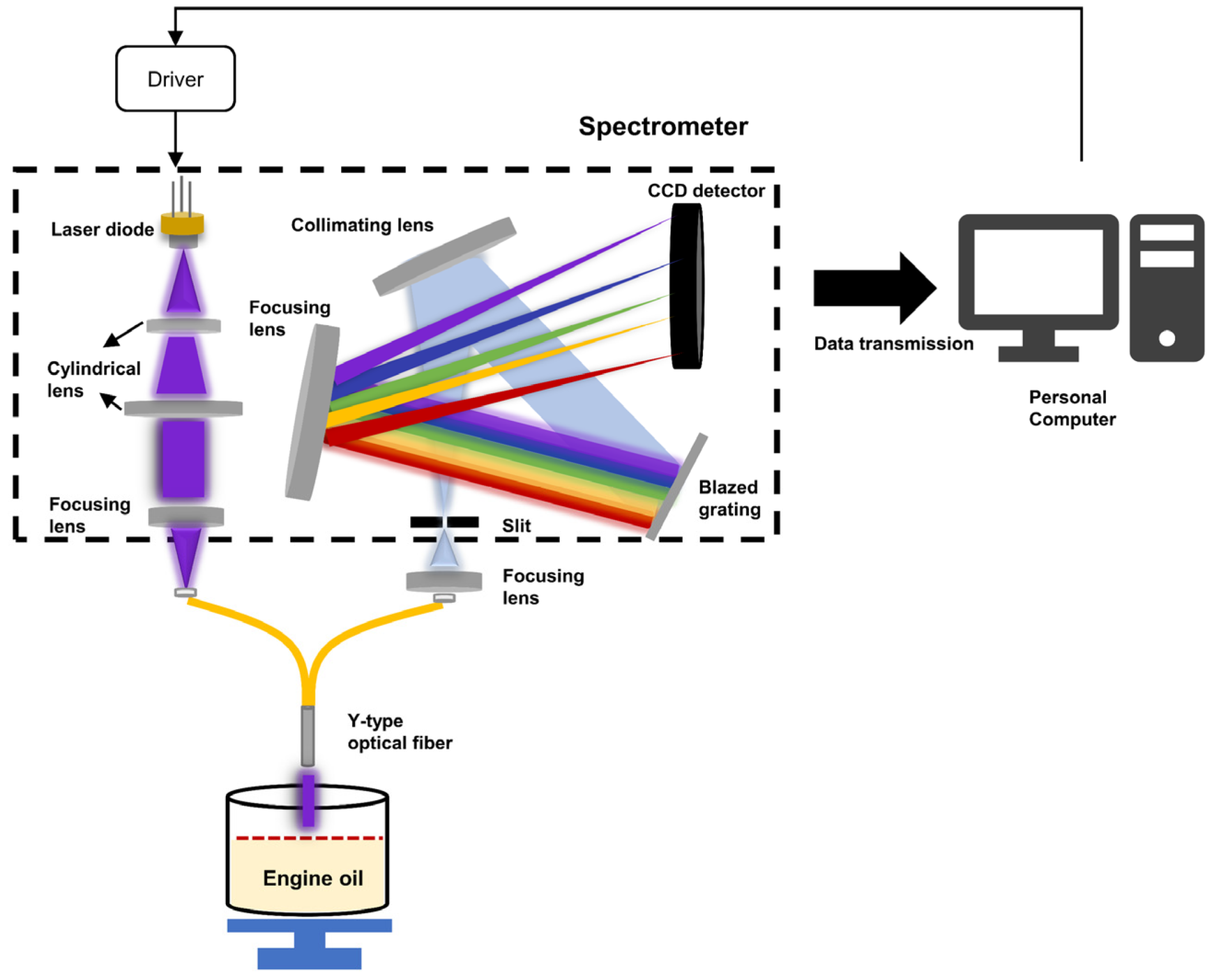
2.1. Data Acquisition

The fluorescence spectra used to train and test the machine learning model were obtained under controlled laboratory conditions. The experimental samples are categorized into seven groups, consisting of three types of oils: Shell Helix 5W-40 (manufactured by Shell plc, Beijing, China), Mobil Super 1000 X1 Diesel 15W-40 (manufactured by ExxonMobil Corporation, Shanghai, China), and Mobil Super 4T 20W-50 (manufactured by ExxonMobil Corporation, Shanghai, China), as well as several 1:1 volume mixtures of these oils: Shell Helix 5W-40 + Mobil 15W-40, Shell Helix 5W-40 + Mobil 20W-50, Mobil 15W-40 + Mobil 20W-50, and Shell Helix 5W-40 + Mobil 15W-40 + Mobil 20W-50. It should be noted that in real-world scenarios, oil mixtures often exhibit unknown and highly variable proportions, making it challenging to obtain representative data for such mixtures. Due to these limitations, we adopted a 1:1 volumetric ratio as a simplified and controlled experimental design to serve as a substitute for actual mixtures. This approach ensures that the fluorescence characteristics of the mixed components can be sufficiently captured and allow for the clear evaluation of spectral differences between pure and mixed oils. While this idealized design does not fully replicate the complexity of real-world conditions, it provides a feasible and effective method for validating the sensitivity of a fluorescence spectroscopy to compositional differences under controlled laboratory conditions.

These oils differ in their applications, resulting in variations in viscosity, appearance, and chemical composition, which are reflected in their fluorescence spectra through differences in intensity, shape, and peak positions. Each sample was prepared in a volume of 100 mL and placed in a beaker. The experimental setup consisted of three main components: a miniature spectrometer, a Y-type optical fiber, and a personal computer. A 405 nm pulsed laser with adjustable power was directed vertically onto the sample surface via a 600 μm core diameter fiber. The fiber probe was positioned 5 cm above the oil samples. Fluorescence emitted from the sample was transmitted back to the spectrometer for spectral separation and sent to the computer for further analysis. The self-made portable fluorescence spectrometer used in this study is capable of emitting a 405 nm laser with powers ranging from 1 to 100 mW. It features a blazed grating for dispersion, covering a spectral range of 400–800 nm with a resolution of approximately 0.5 nm. The spectrometer is equipped with Hamamatsu TDI-CCD image sensors (manufactured by Hamamatsu Photonics (China) Co., Ltd., Shanghai, China), renowned for their high sensitivity and low noise performance, enabling precise capture of spectral variations. The laser source is a Thorlabs 405 nm laser diode (Thorlabs Inc., Newton, NJ, USA), featuring an adjustable pulse width ranging from 500 ns to 5 µs and a maximum repetition rate of 100 kHz.

The schematic diagram of the measurement system is shown in Figure 1. The measurement system consists of a transmission system and a reception system. The transmission system includes a laser diode and a laser collimation system. The driving system controls the laser diode to activate at fixed time intervals, while a cylindrical lens corrects the divergence angle of the laser diode to ensure uniform energy distribution during beam propagation. Finally, the beam is coupled into an optical fiber through a focusing lens. The reception system comprises a dispersion unit and a signal reception unit. A crossed Czerny-Turner (CT) optical path is used to disperse the received fluorescence signal. This design offers advantages such as a compact structure and a short optical path, making it suitable for miniaturized spectrometers. For the signal reception unit, a control module synchronizes the laser and CCD, enabling the CCD camera to perform two measurements within a single laser cycle, thereby achieving background correction. Each scan takes approximately 500 milliseconds. The spectrometer’s range covers the entire visible spectrum, which aligns with the fluorescence peaks of petroleum products excited by the 405 nm laser.

Previous studies have discussed how factors like detector angle, sample distance, and stability affect fluorescence intensity [36], but the influence of laser power on spectral shape has not been fully investigated. The influence of laser power on the fluorescence spectra is a critical factor in spectral analysis. As the laser power increases, the intensity of the fluorescence signal typically increases. However, this also affects the spectral shape in several ways. Specifically, higher laser power can lead to fluorescence saturation, especially in compounds with strong fluorescence emission characteristics. For instance, polycyclic aromatic hydrocarbons (PAHs), commonly found in petroleum products, exhibit intense fluorescence peaks at specific wavelengths. When the laser power is too high, these peaks may become saturated, causing a flattening of the spectral curve and a loss of finer spectral features. This saturation effect can obscure key distinctions between similar substances, making accurate classification more challenging. In real-world detection scenarios, the relative distance between the detector and the oil spill often fluctuates due to wave action. For example, during shipborne or drone-based close-range spectral acquisition, even with constant laser power, saturation may occur when the detection fiber is too close to the oil spill, even at low laser power. Conversely, at greater distances, a strong laser power may still result in weak fluorescence signals. Under conditions of strong wave action, the fluctuations in the detection distance can lead to saturation in the measured fluorescence spectra. Spectra collected under laboratory conditions that assume standard scenarios may fail to account for these effects, leading to model failure in practical applications. Therefore, when collecting oil spectra, it is essential to consider the combined influence of detection distance and laser power on model accuracy.

Since our experiments were conducted in a static environment where the relative distance between the detector and the oil spill remained constant, we introduced simulated wave effects to examine their impact on spectral acquisition and ensure the model’s practical applicability. To this end, we set the laser power to 5 mW, 20 mW, 40 mW, and 60 mW, collecting 30 samples for each power level. Each sample was scanned for 5 s, and the final spectrum was derived from the average of 10 consecutive scans. The sample position was continuously adjusted during data collection. Since a total of 120 spectra were acquired for each substance at four distinct laser power levels, the original spectral dataset comprises 840 spectra corresponding to seven substances. Figure 2 shows the fluorescence spectra of several samples at the four different laser power levels. The figure shows that the fluorescence spectra of pure and mixed oils differ due to variations in their chemical compositions. On a microscopic level, these differences reflect disparities in molecular energy levels, resulting in variations in fluorescence intensity, characteristic peaks, spectral shapes, and spectral decay trends. Even if these differences are not readily apparent in the raw spectra, they may become more pronounced after applying first-order and second-order derivatives to the spectral data. In Figure 2a, the fluorescence peaks of the samples are primarily concentrated at around 500–550 nm, with notable differences in intensity and the peak ratios near 475 nm and 540 nm. As the laser power increases, the spectra of the samples broaden and become more similar, which can be attributed to the saturation effects. At the 5 mW laser power setting, distinct differences in the spectral shape of pure oil samples are evident, while the spectra of the mixed samples share similar shapes with varying intensities. As laser power increases, the spectra broaden, and the differences between them diminish. At 60 mW, the fluorescence spectra of all samples are nearly identical, which is likely due to the saturation of the fluorescence signal. This observation suggests that training a machine learning model exclusively on spectra with pronounced features may render it ineffective in handling the spectral variations caused by differences in laser energy and detection distance during real-world detection.

Thus, collecting fluorescence spectra at varying laser powers, as demonstrated in Figure 2, is one of the data augmentation strategies used in this study to increase the dataset’s diversity and improve the model’s robustness. These power levels were chosen to cover key spectral conditions, including clear fluorescence peaks and complete saturation of the fluorescence signal. While the power levels were discrete, they effectively represent the potential range of spectral variations that may occur under real-world conditions. This approach helps simulate real-world variations in laser power and detection distance, ensuring that the model can adapt to spectral changes arising from fluctuations in laser intensity and detection distance. The model’s ability to accurately classify oil samples under varying laser power conditions demonstrates the effectiveness of this method in enhancing classification performance.

2.2. Data Preprocessing and Augmentation

During the testing spectra may be affected by measurement errors from sources such as ambient light, instrument inaccuracies, or environmental disturbances, introducing noise or other disruptive signals into the acquired spectra [15,21]. Traditional chemometric analysis methods often rely on combinations of preprocessing techniques to filter out noise and improve the signal-to-noise ratio. In this study, we applied Savitzky–Golay (SG) filtering [37] and Standard Normal Variate (SNV) [38] methods to remove noise and correct spectral distortions caused by surface scattering. Additionally, we normalized the spectra to unify intensity distribution across all samples, which facilitated subsequent data processing and minimized the influence of intensity variations on model decisions. This is important since in real measurements, the intensity of spectra can vary due to the movement of the oil spill area.

One key aspect of data augmentation in this study is to simulate real-world variations in the spectral data, which helps the model generalize better across different operational conditions. Recognizing that sample diversity can impact model performance, we performed data augmentation on the dataset. Following Bjerrum et al. [39], we applied multiplication, noise addition, and random shift transformations to the dataset.

Multiplication was adjusted using ±0.1 times the standard deviation of the training set, with slopes uniformly adjusted between 0.95 and 1.05. This helps simulate variations in the spectral intensity, accounting for changes in sensor sensitivity or ambient light conditions. Noise addition ranged from 1% to 5% of the standard deviation of the training data. This technique introduces variability that helps the model generalize noisy data, which is common in real-world spectral measurements due to environmental interference and measurement inaccuracies. Random shifts were limited to occur within 5 nm to simulate differences in spectral calibration among instruments. This mimics potential misalignments in the instrument’s wavelength calibration during spectral acquisition, ensuring the model adapts to variations in spectral baselines. The dataset was randomly divided into training, validation, and test sets in a 3:1:1 ratio. For each training sample, this process was repeated nine times, expanding the dataset from the original 840 to 5376 samples. The resulting augmented dataset provides a more comprehensive representation of the spectral variability that the model may encounter during real-world deployment, improving its generalization capabilities.

2.3. ResNet-LSTM-Attention Network Model

In recent years, convolutional neural networks (CNNs) have demonstrated exceptional feature extraction and learning capabilities, leading to their widespread use in spectral recognition. However, CNNs excel at extracting local features from data arrays, such as images, by isolating important regions and enhancing model accuracy and efficiency. For spectral data, which is a one-dimensional sequence, its features often exhibit both local and global correlations. Therefore, it is crucial to develop a deep learning model capable of extracting these local and global relationships in a manner consistent with the physical mechanisms of spectroscopy, rather than merely applying various mathematical transformations to the spectral data. Thus, we propose a novel deep learning model based on the ResNet architecture, named the ResNet-LSTM-Attention Network (RLANet). This model integrates CNN, LSTM, and Attention modules, using ResNet’s residual connections to extract local fingerprint information from fluorescence spectra while preserving global information. LSTM is used to learn long-range dependencies in the spectral data at different wavelength intervals, and Multihead Attention establishes local and global connections, capturing more sequential relationships and improving LSTM processing efficiency. Additionally, GAP is employed to compress data dimensions while retaining global spectral features, eliminating the need for fully connected layers. Zhang et al. [40] were the first to apply the GAP layer in CNN models for spectral analysis, enhancing model interpretability through class activation methods. GAP is a unique form of average pooling that reduces data dimensionality by compressing each feature map into a single average value. Unlike max pooling, GAP preserves more spectral information while reducing model complexity and mitigating overfitting risks [41].

Figure 3 shows the model architecture. The entire model consists of three ResNet blocks, one LSTM block, and one Multihead Attention block. Spectral data are passed through two different scales of convolution in each ResNet block, summed with the original spectral data, and passed to the next layer. After three ResNet blocks, GAP compresses the features, which are then sent to the LSTM and Multihead Attention layers to extract local and global feature connections. Finally, concatenation and a linear layer transform the features before passing them through a SoftMax layer for output normalization, converting the network’s output into a probability distribution. Compared to traditional deep learning models, our proposed RLANet offers the following advantages:

(1)

Comprehensive feature extraction: ResNet captures local spectral features, LSTM handles long-term dependencies, and Multihead Attention flexibly focuses on different feature regions. This combination enables the model to extract both global and local features, surpassing CNNs and other models limited to local patterns.

(2)

Efficient parameter utilization: GAP reduces model parameters and improves training speed by replacing fully connected layers, making the model computationally efficient and suitable for resource-constrained applications.

(3)

Handling long sequences: LSTM excels in processing temporal information in spectra, capturing complex dependencies. This makes it particularly suitable for sequential data like spectra, outperforming traditional deep learning models such as CNN and MLP in processing long sequences.

(4)

Stronger generalization and robustness: The Attention mechanism enhances model robustness in noisy or diverse data by focusing on different features using multiple heads. GAP also reduces model parameters, minimizing overfitting risk and improving performance in both test and real-world environments.

2.4. Model Implementation

The selection of hyperparameters is crucial to the performance of deep learning algorithms. Traditional trial-and-error approaches, or model improvements based on image processing, are not ideal for selecting parameters for 1D spectral deep learning models. Passos et al. [42] and Mishra et al. [43] highlighted that appropriate hyperparameter selection can reduce model complexity and improve convergence speed in deep learning models for spectral analysis. Currently, the most common method for hyperparameter optimization is the Bayesian Optimization (BO) algorithm. BO is a global optimization method that uses probabilistic models and is often applied to optimize expensive-to-evaluate black-box functions. It builds a probabilistic model of the objective function, allowing it to efficiently select promising sample points and reduce unnecessary computations [44]. Dirks and Poole [45] used Bayesian methods to optimize parameters such as the number of fully connected layers, kernel numbers, and kernel widths, successfully identifying the best solution. Passos et al. [42] proposed a specific method for optimizing deep learning hyperparameters using BO. Although BO is widely used in hyperparameter tuning for deep learning, it struggles with high-dimensional data, which increases the dimensionality of the search space and can limit BO’s performance. Furthermore, its limited parallelization capability—usually sampling one point per iteration based on the acquisition function—constrains its efficiency in large-scale deep learning experiments. This makes BO less efficient when dealing with the large hyperparameter search spaces typical of deep learning models, as it cannot fully leverage modern multi-core or distributed computing architectures. These challenges can hinder the efficiency of hyperparameter optimization, particularly in large and complex deep learning models [46].

In this study, we employed a novel metaheuristic optimization method—the Kepler Optimization Algorithm (KOA)—to optimize various hyperparameters of the RLANet model. To the best of our knowledge, this is the first time KOA has been introduced to optimize deep learning models. Mohamed et al. [47] introduced KOA as a physics-based metaheuristic algorithm, inspired by Kepler’s laws of planetary motion. KOA simulates celestial movement, where each planet and its position serve as candidate solutions. Through random updates relative to the best solution (the Sun), KOA achieves global exploration and local exploitation of the solution space, eventually converging near the global optimum. This is achieved through the interaction of two primary forces:

(1)

Gravitational Attraction: Each candidate solution (planet) is attracted to the best solution (the Sun), helping it explore the solution space and find areas with potential global optima.

(2)

Orbital Motion: Similarly to how the planets orbit the Sun, the candidate solutions undergo random movements that allow for the simultaneous exploration of multiple regions of the solution space.

We used KOA to optimize a set of critical hyperparameters that directly impact the performance of RLANet. These hyperparameters include the learning rate, batch size, kernel sizes, strides, number of layers (CNN block), LSTM hidden units, number of layers (LSTM), epochs and number of attention heads. Each of these hyperparameters was treated as a “planet” in the KOA framework. The initial population of candidate solutions (planets) was randomly generated across the possible ranges for each hyperparameter. As the KOA progressed, each planet (hyperparameter combination) was updated based on the gravitational pull of the best solution (optimal hyperparameter configuration). This process allowed the KOA to explore the search space efficiently while converging towards the best combination of hyperparameters.

The steps for applying KOA to hyperparameter optimization are as follows:

(1)

Initialization: The algorithm initializes a population of candidate solutions (hyperparameter configurations). For instance, the learning rate might be initialized within the range [1 × 10⁻⁵, 1 × 10⁻²], batch size within [16, 32, 64, 128, 256, 512], and the kernel size varied between [3, 21]. These initial solutions are evaluated based on the model’s performance using a validation set.

(2)

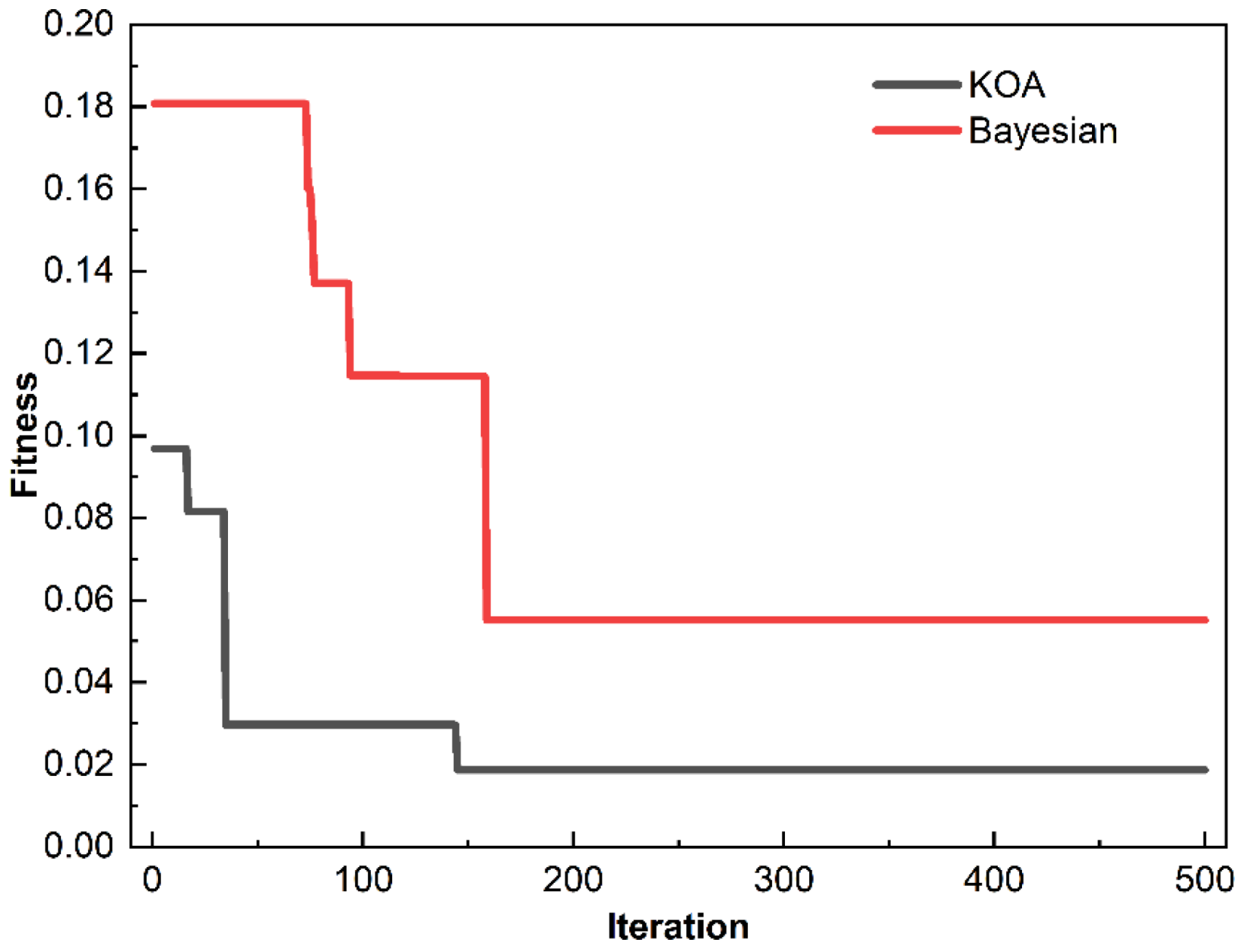
Gravitational Update: Each candidate solution (planet) is updated by being attracted to the best solution (the Sun). The quality of each candidate solution is evaluated based on the model’s performance (average loss rate of the training and validation sets) and its distance from the best solution. The gravitational force draws the candidate solutions toward regions of the solution space with the highest-quality configurations (e.g., optimal learning rates, batch sizes, etc.). This process ensures that the algorithm focuses on areas of the search space with the most promising hyperparameter configurations.

(3)

Orbital Adjustment: To explore the solution space more broadly and avoid getting trapped in local optima, the candidate solutions undergo orbital adjustments. This allows the algorithm to explore multiple regions of the solution space simultaneously. For example, the kernel size may need to vary more widely to capture features at different scales, and the batch size may need to be fine-tuned to balance computational cost with model performance. The orbital motion ensures that the solutions do not become overly focused on a small region of the search space, promoting a more thorough exploration.

(4)

Parallelization: Unlike BO’s sequential approach, KOA supports parallel computation, allowing multiple candidate solutions to be evaluated at once. This is particularly useful when dealing with a large number of hyperparameter configurations. For example, KOA can evaluate various combinations of learning rate, batch size, and kernel size simultaneously, significantly speeding up the optimization process. In deep learning tasks like RLANet, with high-dimensional hyperparameter spaces, this parallelism is especially beneficial for efficiently exploring the search space and finding optimal solutions faster.

Compared to BO, KOA offers several key advantages:

(1)

Global and Local Search: KOA combines gravitational attraction with orbital motion, allowing it to search the solution space more broadly and effectively than BO. This reduces the risk of getting stuck in local optima and enhances the algorithm’s robustness in high-dimensional spaces.

(2)

Parallelization: Unlike BO’s sequential approach, KOA supports parallel computation by evaluating multiple candidate solutions simultaneously. This makes KOA particularly well-suited for deep learning tasks, where large hyperparameter search spaces need to be explored efficiently and at scale.

(3)

Scalability: KOA’s parallelism and efficient global search make it scalable to larger models and datasets, which is a key advantage over BO when optimizing hyperparameters in complex deep learning models, like RLANet.

After optimization, the best hyperparameters were used for model training. We used cross-entropy loss function [48] to calculate the loss rate and adopted the Adam method as the optimizer. Compared to other adaptive algorithms like Stochastic Gradient Descent (SGD) [49], the Adam method dynamically adjusts the learning rate for each parameter using first-order and second-order moment estimates of the gradient [50]. After bias correction, each iteration’s learning rate is bound, leading to more stable parameters. To enhance model performance and avoid overfitting, we monitored overfitting using validation set performance. The training process was executed on an NVIDIA GTX-3090 GPU in a CUDA 11.8 and cuDNN 8.7.0 environment. The implementation code for our proposed method was written in Python 3.10.10 using PyTorch 2.0.0.

3. Results and Discussion

3.1. Neural Network Training Process

Table 1. Hyperparameter Optimization Results.

Hyperparameter	Range/Values	Optimal Solution (KOA)	Optimal Solution (BO)
Learning rate	[1 × 10−5, 1 × 10−2]	3.363 × 10−5	6.725 × 10−5
Number of Layers (CNN Block)	[2, 5]	3	3
Batch size	[16, 32, 64, 128, 256, 512]	128	512
Kernel sizes	[3, 21]	[21, 11, 11]	[21, 3, 15]
Strides	[1, 5]	[4, 3, 3]	[4, 5, 2]
LSTM hidden units	[8, 16, 32, 64, 128, 256, 512]	32	32
Number of layers (LSTM)	[1, 5]	2	2
Number of attention heads	[2, 16]	6	10
Epochs	[50, 100, 200, 300, 400, 500, 600, 700]	500	500

displays the hyperparameter optimization results for deep learning models using the KOA and BO methods. For KOA, the initial number of search planets was set to 20, with 500 iterations; BO was similarly set to 500 iterations. As shown in Table 1, the main differences in parameter optimization between the two methods are found in kernel size, stride, and batch size, while other parameters are relatively similar. KOA’s selection of kernel size and stride appears more reasonable. A larger kernel size in the first convolution layer captures important feature regions while filtering out redundant points, followed by smaller kernels to further increase the receptive field—this approach aligns with existing spectral deep learning models. In contrast, BO results in less optimal parameters, particularly in choosing a batch size that increases computational burden. KOA’s selection of batch size (128) results in a more balanced optimization, reducing computational costs without sacrificing performance. Figure 4 depicts the fitness curves for both methods over 500 iterations. The fitness value is calculated as the weighted average of the training and validation loss functions; the smaller the fitness value, the smaller the overall loss. From Figure 4, it is evident that KOA achieves a fitness value of about 0.018 after 500 iterations, which is significantly lower than the BO method’s fitness value of only 0.055 after the same number of iterations. Additionally, KOA’s initial fitness value is lower, leading to faster convergence, thanks to its broader global search capability.

The results demonstrate that the model achieves optimal fitness around 500 epochs. However, due to the inherent nonlinearity and instability in deep learning model training, excessive training can lead to overfitting. To determine the optimal number of epochs, both optimized models were trained 50 times, with epoch counts ranging from 300 to 700. The optimal epoch was selected based on the accuracy and stability of both the training and validation sets. As shown in

Table 2. KOA-RLANet and BO-RLANet Model Performance.

Method	Epochs	Accuracy (Train)	Std (Train)	Loss Rate (Train)	Accuracy (Valid)	Std (Valid)	Loss Rate (Valid)
KOA-RLANet	300	0.9985	0.0009	0.0098	0.9772	0.0059	0.083
	400	0.9987	0.0009	0.0058	0.9760	0.0082	0.0902
	500	0.9988	0.0012	0.0037	0.9793	0.0052	0.0785
	600	0.9988	0.0008	0.0026	0.9743	0.0167	0.0973
	700	0.9987	0.0009	0.0019	0.9771	0.0083	0.0837
BO-RLANet	300	0.9843	0.0076	0.0830	0.9647	0.0081	0.1522
	400	0.9884	0.0048	0.05	0.9631	0.0216	0.1558
	500	0.9899	0.0043	0.0367	0.9694	0.0101	0.1274
	600	0.9904	0.0058	0.029	0.9641	0.0327	0.1496
	700	0.9912	0.0034	0.0235	0.9690	0.0113	0.1322

, KOA-RLANet achieves stable accuracy on the training set at around 500 epochs, with a decreasing standard deviation across multiple trials. Performance on the validation set also peaks at 500 epochs but declines with further training, indicating potential overfitting. For BO-RLANet, a similar trend was observed, but its overall performance was lower than KOA-RLANet, consistent with the results shown in Figure 4. Figure 5 depicts the loss and accuracy curves for both optimization methods over different epochs. The model optimized using the KOA converged faster, with the training and validation losses falling below 0.2 by 100 epochs and stabilizing at around 500 epochs. In contrast, BO-RLANet exhibited slower convergence and suboptimal performance compared to KOA-RLANet, highlighting that the parameters optimized by KOA are more appropriate. Furthermore, the optimal solution obtained with the same number of iterations was superior when using the KOA. Therefore, the final parameter settings for the RLANet training network are based on the KOA optimization results. For clarity, subsequent references to RLANet will refer to the model optimized by KOA.

To further highlight our model’s advantages, we trained four other deep learning models commonly used in spectral and time-series analysis: CNN, LSTM, GRU, and RNN, with hyperparameters optimized via KOA. Figure 6 shows the training process for these models. Among them, CNN performed best, achieving stable results after 1000 epochs, comparable to RLANet. However, CNN’s reliance on fully connected layers introduces a significant increase in computational complexity and risk of overfitting, especially when applied to large datasets. Among the models, RNN performed the worst. Its convergence speed was slow, stabilizing only after around 3000 epochs. However, its performance on both the training and validation sets was significantly lower than that of RLANet and CNN. This is because RNN, an earlier model for sequence data, mainly relies on updating from the previous step to the next, which makes it ill-suited to handle long-sequence data such as spectra. Furthermore, RNN suffers from the vanishing gradient problem [51], which contributes to its poor performance in our task. The GRU model performed slightly better than the RNN model, achieving about 80% accuracy on the training set and around 70% on the validation set after 3000 epochs. This is because GRU introduces update gates and reset gates, allowing it to selectively retain or forget information [52]. This architecture enables GRU to capture more important information in sequential data and reduce the vanishing gradient problem seen in RNNs. However, for spectral data, the simple gating mechanism of GRU is insufficient for capturing long-term dependencies. Compared to RNN and GRU, LSTM performed better. Due to the introduction of memory cells and a more complex gating mechanism, LSTM is more stable when handling long-sequence data. After 5000 epochs, LSTM achieved more than 80% accuracy on both the training and validation sets. However, because LSTM’s gate mechanism is more complex, it has a larger number of parameters, which means the model requires more time to adjust its weights and converge, thus requiring more epochs to achieve optimal performance.

Table 3. Performance of RLANet, CNN, LSTM, GRU, and RNN models on the test set.

Method	Accuracy	Steady Iteration	Time	Parameter
RLANet	99.51%	500	1 min 12 s	0.09 M
CNN	99.40%	1000	3 min	11.35 M
LSTM	89.73%	5000	12 min 40 s	4.57 M
GRU	81.18%	3000	7 min 8 s	1.52 M
RNN	78.76%	3000	5 min 15 s	0.64 M

presents the performance of all five models on the test set, showing the number of iterations required to stabilize, the training time, and the number of parameters for each model. As shown in Table 3, our proposed RLANet model achieved 99.51% accuracy on the test set, significantly higher than the LSTM, GRU, and RNN models. Moreover, RLANet required fewer training epochs and less training time, indicating lower computational complexity. This is attributed to the use of GAP and the Attention mechanism. The Attention mechanism dynamically assigns weights to input features, effectively reducing redundant computations, while GAP replaces the traditional fully connected layer, greatly reducing the number of parameters in the model. Despite achieving similar accuracy, CNN’s larger number of parameters and complexity make it less suitable for deployment on resource-constrained devices, which are common in real-time applications. The comparison in Table 3 clearly shows that our proposed model not only guarantees high accuracy but also has fewer parameters and lower computational overhead. This suggests that RLANet has a lower computational burden and can be deployed on hardware with limited resources for real-time detection.

In addition, we acknowledge the accuracy and widespread adoption of CNN in various fields. However, RLANet is specifically designed to address the challenges of real-time prediction and resource efficiency, which are critical for on-site oil spill detection and large-scale spectral monitoring. In these real-world scenarios, RLANet offers a balanced approach between accuracy and computational efficiency, while its very small parameter count allows it to be deployed in environments with limited hardware resources. Therefore, although RLANet’s simplified architecture has comparable accuracy to CNN, it is designed specifically for deploying critical applications in environments with low computational overhead and limited hardware resources.

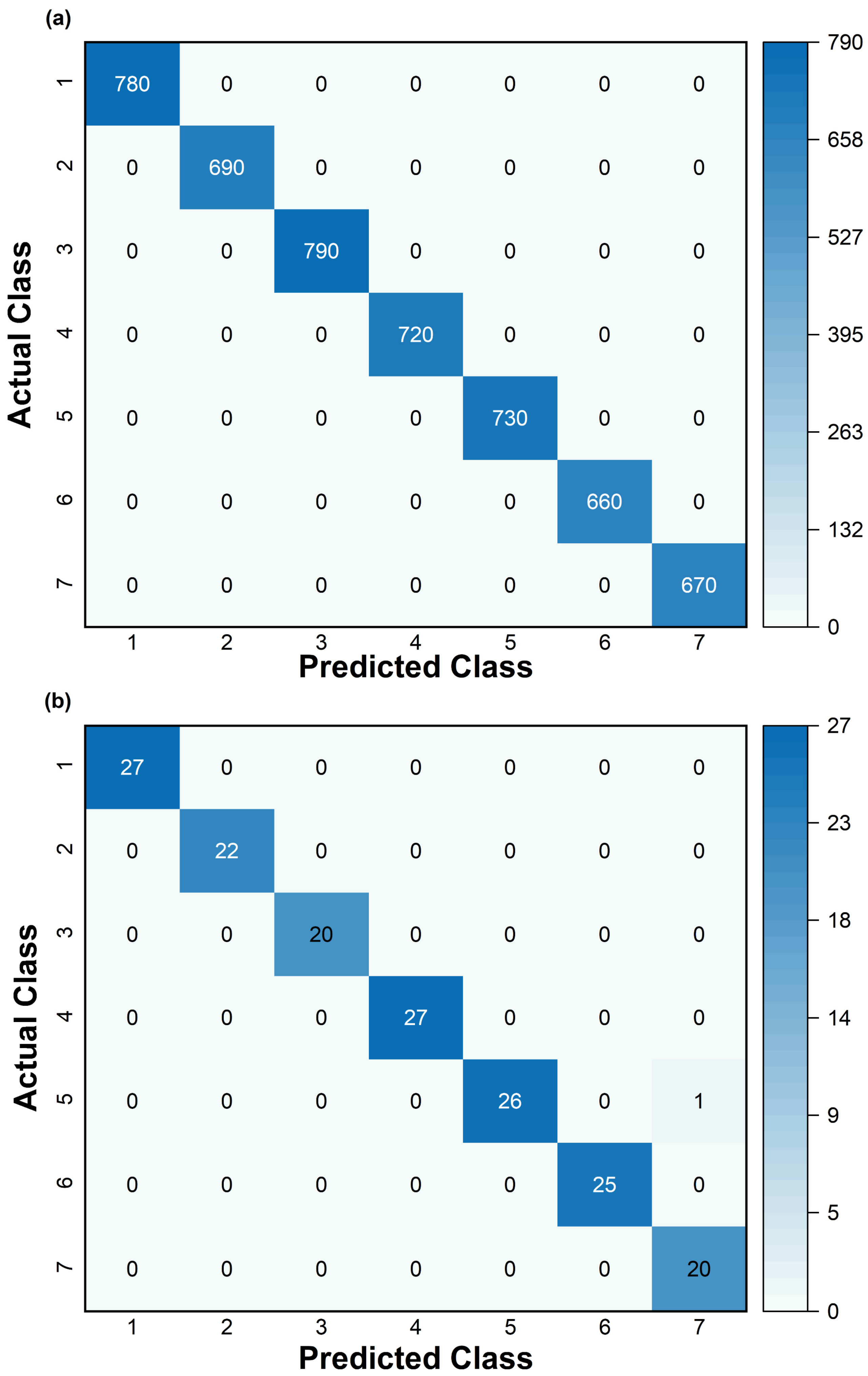
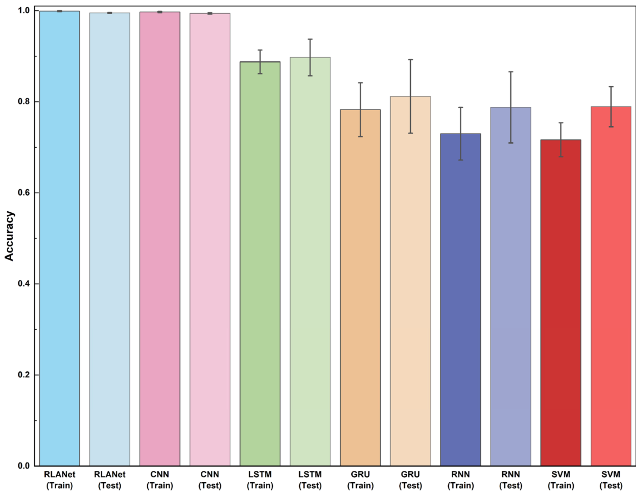
3.2. Classification Performance

After the training process, the performance of the RLANet model was evaluated using both the training and the test sets. The confusion matrix for the spectral classification of the seven substances is shown in Figure 7. Labels 1–7 represent Helix 5W-40, Mobil 15W-40, and Mobil 20W-50, Helix + Mobil 15W-40, Helix + Mobil 20W-50, Mobil 15W-40 + Mobil 20W-50, and Helix 5W-40 + Mobil 15W-40 + Mobil 20W-50. As seen from Figure 7, RLANet achieved perfect classification accuracy for the training set without any errors. For the test set, however, there was one misclassification where the model confused the spectrum of a mixture of Helix 5W-40 and Mobil 20W-50 with the spectrum of a mixture from all brands. As illustrated in Figure 2, the spectra of these two substances differ only in fluorescence intensity while maintaining similar linearity, making misclassification somewhat probable. Nonetheless, only one sample was misclassified, which is acceptable for our model. The confusion matrix indicates that RLANet exhibits excellent classification capability, accurately identifying not only the pure oil spectra but also successfully distinguishing the spectra of mixed oil samples from different brands. This implies that, relying on the diversity of the dataset and the feature learning capabilities of deep learning, the model can correctly identify mixed oil spills in real-world scenarios. Instead of misclassifying them as a single substance, the model recognizes them as mixtures of multiple oil types.

Figure 8 compares the proposed RLANet model with several common deep learning models and a standard chemometric analysis algorithm (SVM) in terms of their average accuracy over 50 repeated training sessions, without any data preprocessing. As shown in Figure 8, the RLANet model achieved nearly 100% accuracy without data preprocessing, with a minimal standard deviation in both the training and test sets, demonstrating the model’s exceptional robustness. The standard deviation of CNN accuracy is slightly larger than that of RLANet, but it remains significantly smaller than the other models. For LSTM, GRU, and RNN, their inherent algorithmic characteristics lead to poorer robustness, making them unsuitable for long-sequence spectral analysis. SVM, due to its iterative optimization process, shows a relatively consistent performance without substantial changes in accuracy when the hyperparameters remain unchanged, with greater stability compared to GRU and RNN.

In traditional spectral analysis models, data preprocessing is often an essential step. Many studies have demonstrated that different combinations of preprocessing techniques can either enhance or degrade model performance [53]. For some deep learning models, especially CNNs, research suggests that convolution operations are similar to preprocessing methods such as SG, thus eliminating the need for explicit preprocessing. To better illustrate the dependency of different models on preprocessing methods, we list the test set performance of several models under various preprocessing methods after 50 repeated training sessions in

Table 4. Accuracy and stability performance of models under different preprocessing methods.

Methods	Raw		SG		SG+SNV		SG+SNV+NORM
RLANet	Best	100%	Best	100%	Best	100%	Best	100%
	Worst	98.81%	Worst	99.40%	Worst	99.40%	Worst	99.35%
	Mean	99.51%	Mean	99.68%	Mean	99.81%	Mean	99.73%
	Std	0.0008	Std	0.0012	Std	0.0008	Std	0.0010
CNN	Best	100%	Best	99.98%	Best	99.98%	Best	99.98%
	Worst	98.81%	Worst	98.79%	Worst	99.09%	Worst	98.81%
	Mean	99.40%	Mean	99.43%	Mean	99.52%	Mean	99.55%
	Std	0.0012	Std	0.0023	Std	0.0024	Std	0.0028
LSTM	Best	97.62%	Best	98.81%	Best	99.40%	Best	88.69%
	Worst	79.76%	Worst	80.95%	Worst	96.43%	Worst	85.71%
	Mean	89.73%	Mean	90.10%	Mean	97.96%	Mean	87.42%
	Std	0.0405	Std	0.0497	Std	0.0075	Std	0.0058
GRU	Best	93.45%	Best	95.83%	Best	80.95%	Best	77.38%
	Worst	60.71%	Worst	64.88%	Worst	72.62%	Worst	73.81%
	Mean	81.18%	Mean	82.89%	Mean	77.32%	Mean	74.61%
	Std	0.0807	Std	0.0730	Std	0.0193	Std	0.0068
RNN	Best	94.05%	Best	86.90%	Best	82.14%	Best	80.95%
	Worst	61.90%	Worst	39.29%	Worst	73.81%	Worst	74.40%
	Mean	78.76%	Mean	67.32%	Mean	78.63%	Mean	77.74%
	Std	0.0781	Std	0.0929	Std	0.0218	Std	0.0141
SVM	Best	87.5%	Best	89.29%	Best	94.04%	Best	89.88%
	Worst	69.04%	Worst	69.64%	Worst	75%	Worst	68.45%
	Mean	78.93%	Mean	78.46%	Mean	85.55%	Mean	81.30%
	Std	0.044	Std	0.0431	Std	0.0483	Std	0.0439

. It is evident that for our proposed RLANet model, performance is largely unaffected by different preprocessing methods, with peak accuracy reaching 100% and average accuracy showing a certain degree of improvement. While the standard deviation shows slight fluctuations, it remains minimal, indicating strong robustness. This suggests that RLANet has a low dependency on preprocessing and exhibits excellent robustness. This robustness can be attributed to the use of the Attention mechanism and GAP in RLANet, which enable the model to effectively capture key spectral features and reduce sensitivity to preprocessing variations. For the CNN model, although the average accuracy improves after preprocessing, the peak accuracy declines, and the standard deviation increases. This indicates that CNN is more sensitive to preprocessing techniques during feature extraction, making its performance less stable under varying preprocessing conditions.

For LSTM, however, performance fluctuates significantly after preprocessing, with a noticeable drop in peak accuracy after the combination of SG + SNV + NORM. We believe this phenomenon is related to the long-term dependency on the processing capabilities of LSTM. Complex preprocessing methods might alter the temporal structure of the data, making it difficult for LSTM to capture long-term dependencies. This suggests that when using sequence-processing models like LSTM, one must carefully select the preprocessing methods to avoid excessively altering the sequential characteristics of the data. Similar fluctuations were observed in the GRU and RNN models, where performance varied considerably after the preprocessing. This indicates that LSTM, GRU, and RNN, which are designed for time-series data, are more sensitive to noise and signal fluctuations, lacking the inherent noise-filtering capabilities of CNN. These models are also highly sensitive to preprocessing combinations, as certain preprocessing steps can introduce additional noise, leading to model degradation. Thus, although spectral and time-series data both take the form of 1D sequences, it is evident from the performance results that using sequence models alone for spectral analysis is insufficient. Network modifications are often needed to enhance feature extraction and robustness. Moreover, the standard deviation of RLANet and CNN models is lower without the preprocessing, but it increases after some preprocessing steps. This could be due to excessive preprocessing introducing additional data variability, spectral information loss, and the attenuation of important features, thereby reducing model stability.

From Table 4, we can see that RLANet achieves very high accuracy on unprocessed data and does not significantly degrade after preprocessing. This demonstrates the model’s strong ability to learn from raw data, reducing the need for complex preprocessing steps and saving computational resources. Although the standard deviation increases slightly after some preprocessing steps, the model’s peak accuracy remains at 100%, indicating that RLANet is highly adaptable to different data processing methods. For the CNN model, performance degradation occurs after applying different steps of data preprocessing. Although its average accuracy improves, its stability declines when facing additional bias introduced by preprocessing. In contrast, RLANet achieves comparable performance with fewer parameters, ensuring both accuracy and robustness, making it more suitable for resource-limited environments. By utilizing GAP and the Attention mechanism, RLANet maintains a high accuracy while reducing the computational load, making it an ideal choice for applications such as industrial oil spill detection and continuous spectral analysis, where real-time results are critical. Therefore, while CNN demonstrates comparable accuracy to our proposed model, RLANet is specifically designed for scenarios where the balance between accuracy and efficiency is more critical than simply achieving maximum accuracy. This design provides a practical solution for real-world operational settings, where computational efficiency and real-time analysis are of paramount importance.

Considering that in practical detection tasks the fluorescence signals from oil spills are subject to cumulative interference from various factors, such as ambient light, wave effects, and instrument noise, it is essential to evaluate the model’s robustness. To simulate the interference experienced in real marine environments, noise was added to the test set at signal-to-noise ratio (SNR) levels of 15 dB, 20 dB, 25 dB, and 30 dB, thereby quantifying the noise resilience of the RLANet model in practical applications. Figure 9 presents a representative spectral image of a Mobil 15W-40 sample from the test set after noise at various power levels was introduced. It can be observed that at SNR of 15 dB and 20 dB, the noise significantly distorts the spectrum, nearly obliterating the fluorescence features present in the original signal. Only when the SNR reaches 30 dB do the intrinsic spectral characteristics re-emerge.

Table 5. Classification performance of RLANet model under different noise power levels.

Model	SNR (dB)	Accuracy	Precision	Recall	F1-Score
RLANet	GT	0.994	0.9932	0.9947	0.9938
	15	0.8036	0.8043	0.8058	0.8041
	20	0.8988	0.9006	0.9026	0.9004
	25	0.9583	0.9576	0.9574	0.9574
	30	0.994	0.9949	0.9947	0.9947

summarizes the classification outcomes of the RLANet model on the test set under these different noise conditions. Here, “GT” denotes the model’s performance in the absence of noise. Precision measures the accuracy of the model in predicting positive samples, while Recall indicates the proportion of actual positive samples that are correctly identified, reflecting the model’s completeness. The F1 Score, which is the harmonic mean of precision and recall, is commonly used as an overall performance metric for classification models with values ranging from 0 to 1. Higher values indicate superior performance. The results reveal that the RLANet model exhibits strong robustness to noise-induced spectral perturbations. Even under severe noise interference at an SNR of 15 dB, the model maintains an accuracy above 80% on the test set, with its classification accuracy declining by only approximately 19% compared to the baseline model. Moreover, as signal quality improves, the classification capability of RLANet rapidly recovers, achieving a performance nearly identical to the noise-free scenario at an SNR of 30 dB. These findings demonstrate that our designed RLANet model, through the effective integration of CNN, LSTM, and multihead Attention mechanisms, acquires a deeper understanding of spectral feature distributions. Consequently, the model exhibits a robust performance in the face of signal perturbations caused by various environmental factors, thereby significantly enhancing the interference resistance of LIF technology in real-world conditions and improving its overall practical applicability.

Of course, our current model has certain limitations. The model’s ability to identify mixtures relies on assigning specific labels to mixtures composed of different pure oils during spectral dataset preparation, enabling supervised learning. This means that when the model encounters spectral data from mixtures composed of oils already present in the dataset, it can accurately identify the components rather than misclassifying the mixture as a single substance. However, the model’s generalization capability depends heavily on the diversity of the dataset. If the model encounters petroleum products or mixtures not included in the dataset, it may fail to perform accurately. Moreover, additional factors such as different detectors, water quality, and temperature can significantly influence oil spill spectra, and these were not fully addressed in this study.

The dataset used in this study includes fluorescence spectra collected under controlled laboratory conditions, where 1:1 volumetric mixtures were chosen as a simplified and controlled experimental design. While this design ensures that the fluorescence characteristics of the mixed components are sufficiently captured, it does not fully replicate the complexity of real-world scenarios. In actual spill events, oil mixtures often exhibit unknown and highly variable proportions, as well as additional influencing factors such as fluctuations in sample composition or the complex chemical nature of spilled oils. These real-world variations were not represented in the dataset, which limits the study’s applicability to practical scenarios. Nonetheless, the results obtained from this controlled experiment demonstrate the sensitivity of fluorescence spectroscopy to compositional differences and provide a feasible method for validating the potential of deep learning-based spectral analysis in distinguishing pure and mixed oils.

Future work will focus on integrating unsupervised and transfer learning techniques to reduce the model’s dependency on specific datasets. This would enable the model to effectively learn the patterns of spectral variations in oil mixtures, regardless of the complexity of their compositions. Additionally, more realistic simulations of real-world conditions in laboratory environments, considering diverse influencing factors such as different detectors, water quality, and temperature, will be conducted. For example, future experiments will introduce dynamic setups to modulate the detection distance in real-time, simulating wave-induced fluctuations more accurately. We also plan to refine the experimental design by incorporating more gradations in laser power or continuously varying power levels to better mimic real-world fluorescence intensity fluctuations. Collecting additional spectral data from real-world oil spill scenarios, including mixtures with unknown and variable compositions, will further enhance the model’s applicability and robustness. These efforts will address the current limitations of the dataset and help establish a more comprehensive framework for applying fluorescence spectroscopy and machine learning to complex, real-world oil spill detection scenarios.

4. Conclusions

In this study, we propose a novel deep learning model, RLANet, tailored for spectral analysis. The model combines ResNet, LSTM, and multihead Attention mechanisms, and introduces the KOA for hyperparameter tuning in deep learning for the first time. Our experimental results show that RLANet outperforms traditional deep learning models and chemometric analysis models (CNN, LSTM, RNN, GRU, and SVM) in the spectral classification of petroleum products and their derivatives. RLANet excels in distinguishing pure substances and identifying mixtures, as demonstrated under simplified and controlled experimental conditions. While these conditions do not fully replicate the complexity of real-world scenarios, the results validate the potential of a fluorescence spectroscopy combined with deep learning for addressing more complex real-world challenges.

By eliminating the need for traditional, fully connected layers, RLANet significantly reduces the number of model parameters while maintaining its ability to extract global spectral features. This lightweight and computationally efficient design makes the model particularly suitable for real-time applications in resource-constrained environments. Additionally, the model achieves a robust performance without requiring complex preprocessing, unlike other deep learning models such as CNNs, which exhibit instability when dealing with noisy data or inappropriate preprocessing. By effectively extracting features directly from raw data, RLANet demonstrates superior adaptability and efficiency compared to traditional methods. Robustness testing results indicate that the model’s performance degrades by only 19% under a noisy environment with an SNR of 15 dB, suggesting that our proposed fusion network architecture design strategy enables the model to learn the spectral distribution at a deeper level, thereby conferring strong interference resistance in practical tests.

While this study demonstrates the effectiveness of RLANet for spectral classification, it also acknowledges the limitations of the dataset and experimental design. The fluorescence spectra were collected under controlled laboratory conditions, with 1:1 volumetric mixtures serving as a simplified experimental design. Although this approach ensures that the fluorescence characteristics of the mixed components are sufficiently captured, it does not fully account for the complexity of real-world oil mixtures, which often exhibit unknown and highly variable compositions. Future work will focus on expanding the dataset to include real-world oil spill scenarios and incorporating factors such as water quality, temperature, and detector variability to enhance model robustness. Moreover, integrating unsupervised and transfer learning techniques will further reduce the model’s dependency on specific datasets, enabling it to generalize more effectively to diverse real-world conditions. Enhanced experimental designs, such as incorporating more dynamic and continuous variations in detection conditions, will also improve the model’s applicability to practical scenarios.

In summary, RLANet performs excellently in both pure and mixed oil spectrum classifications. By adapting to complex and diverse oil mixtures, regardless of their compositions, the model demonstrates significant potential for addressing real-world challenges in spectral analysis. Its lightweight and computationally efficient design, combined with the ability to function without complex preprocessing, makes it highly suitable for large-scale real-time applications, such as industrial oil contamination detection and mixture spectrum analysis. Leveraging the KOA for hyperparameter optimization and innovative architectural choices, RLANet represents a smart and efficient solution for advancing spectral analysis in resource-constrained environments.

References

1. Lourenco, R.A.; Combi, T.; Alexandre, M.D.R.; Sasaki, S.T.; Zanardi-Lamardo, E.; Yogui, G.T. Mysterious oil spill along Brazil’s northeast and southeast seaboard (2019–2020): Trying to find answers and filling data gaps. Mar. Pollut. Bull. 2020, 156, 111219. [Google Scholar] [CrossRef] [PubMed]
2. Oliveira, L.G.; Araújo, K.C.; Barreto, M.C.; Bastos, M.E.P.A.; Lemos, S.G.; Fragoso, W.D. Applications of chemometrics in oil spill studies. Microchem. J. 2021, 166, 106216. [Google Scholar] [CrossRef]
3. Spaulding, M.L. State of the art review and future directions in oil spill modeling. Mar. Pollut. Bull. 2017, 115, 7–19. [Google Scholar] [CrossRef]
4. Laffon, B.; Pasaro, E.; Valdiglesias, V. Effects of exposure to oil spills on human health: Updated review. J. Toxicol. Environ. Health B Crit. Rev. 2016, 19, 105–128. [Google Scholar] [CrossRef] [PubMed]
5. Campelo, R.P.S.; Lima, C.D.M.; de Santana, C.S.; Jonathan da Silva, A.; Neumann-Leitao, S.; Ferreira, B.P.; Soares, M.O.; Melo Junior, M.; Melo, P. Oil spills: The invisible impact on the base of tropical marine food webs. Mar. Pollut. Bull. 2021, 167, 112281. [Google Scholar] [CrossRef] [PubMed]
6. Qayum, S.; Zhu, W.D. An overview of International and Regional laws for the prevention of Marine oil pollution and “International obligation of Pakistan”. Indian J. Geo-Mar. Sci. 2018, 47, 529–539. [Google Scholar]
7. Fingas, M.; Brown, C. Review of oil spill remote sensing. Mar. Pollut. Bull. 2014, 83, 9–23. [Google Scholar] [CrossRef]
8. Patra, D. Applications and New Developments in Fluorescence Spectroscopic Techniques for the Analysis of Polycyclic Aromatic Hydrocarbons. Appl. Spectrosc. Rev. 2003, 38, 155–185. [Google Scholar] [CrossRef]
9. Okparanma, R.N.; Mouazen, A.M. Determination of Total Petroleum Hydrocarbon (TPH) and Polycyclic Aromatic Hydrocarbon (PAH) in Soils: A Review of Spectroscopic and Nonspectroscopic Techniques. Appl. Spectrosc. Rev. 2013, 48, 458–486. [Google Scholar] [CrossRef]
10. Chua, C.C.; Brunswick, P.; Kwok, H.; Yan, J.; Cuthbertson, D.; van Aggelen, G.; Helbing, C.C.; Shang, D. Enhanced analysis of weathered crude oils by gas chromatography-flame ionization detection, gas chromatography-mass spectrometry diagnostic ratios, and multivariate statistics. J. Chromatogr. A 2020, 1634, 461689. [Google Scholar] [CrossRef]
11. Lemkau, K.L.; Peacock, E.E.; Nelson, R.K.; Ventura, G.T.; Kovecses, J.L.; Reddy, C.M. The M/V Cosco Busan spill: Source identification and short-term fate. Mar. Pollut. Bull. 2010, 60, 2123–2129. [Google Scholar] [CrossRef] [PubMed]
12. Leifer, I.; Lehr, W.J.; Simecek-Beatty, D.; Bradley, E.; Clark, R.; Dennison, P.; Hu, Y.; Matheson, S.; Jones, C.E.; Holt, B.; et al. State of the art satellite and airborne marine oil spill remote sensing: Application to the BP Deepwater Horizon oil spill. Remote Sens. Environ. 2012, 124, 185–209. [Google Scholar] [CrossRef]
13. Li, Y.; Yu, Q.; Xie, M.; Zhang, Z.; Ma, Z.; Cao, K. Identifying Oil Spill Types Based on Remotely Sensed Reflectance Spectra and Multiple Machine Learning Algorithms. IEEE J. Sel. Top. Appl. Earth Obs. Remote Sens. 2021, 14, 9071–9078. [Google Scholar] [CrossRef]
14. Fedotov, Y.V.; Belov, M.L.; Kravtsov, D.A.; Gorodnichev, V.A. Laser fluorescence method for detecting oil pipeline leaks at a wavelength of 355  nm. J. Opt. Technol. 2019, 86, 81–85. [Google Scholar] [CrossRef]
15. Xie, M.; Xu, Q.; Xie, L.; Li, Y.; Han, B. Establishment and optimization of the three-band fluorometric indices for oil species identification: Implications on the optimal excitation wavelengths and the detection band combinations. Anal. Chim. Acta 2023, 1280, 341871. [Google Scholar] [CrossRef]
16. Brown, C.E.; Fingas, M.F. Review of the development of laser fluorosensors for oil spill application. Mar. Pollut. Bull. 2003, 47, 477–484. [Google Scholar] [CrossRef]
17. Raimondi, V.; Palombi, L.; Lognoli, D.; Masini, A.; Simeone, E. Experimental tests and radiometric calculations for the feasibility of fluorescence LIDAR-based discrimination of oil spills from UAV. Int. J. Appl. Earth Obs. Geoinf. 2017, 61, 46–54. [Google Scholar] [CrossRef]
18. Hou, Y.; Li, Y.; Liu, Y.; Li, G.; Zhang, Z. Effects of polycyclic aromatic hydrocarbons on the UV-induced fluorescence spectra of crude oil films on the sea surface. Mar. Pollut. Bull. 2019, 146, 977–984. [Google Scholar] [CrossRef]
19. Sun, L.; Zhang, Y.; Ouyang, C.; Yin, S.; Ren, X.; Fu, S. A portable UAV-based laser-induced fluorescence lidar system for oil pollution and aquatic environment monitoring. Opt. Commun. 2023, 527, 128914. [Google Scholar] [CrossRef]
20. Yin, S.; Cui, Z.; Bi, Z.; Li, H.; Liu, W.; Tian, Z. Wide-Range Thickness Determination of Oil Films on Water Based on the Ratio of Laser-Induced Fluorescence to Raman. IEEE Trans. Instrum. Meas. 2022, 71, 3134320. [Google Scholar] [CrossRef]
21. Zhang, S.; Yuan, Y.; Wang, Z.; Li, J. The application of laser-induced fluorescence in oil spill detection. Environ. Sci. Pollut. Res. 2024, 31, 23462–23481. [Google Scholar] [CrossRef] [PubMed]
22. Cortes, C.; Vapnik, V. Support-Vector Networks. Mach. Learn. 1995, 20, 273–297. [Google Scholar] [CrossRef]
23. Zhao, W.-L.; Wang, H.; Ngo, C.-W. Approximate k-NN Graph Construction: A Generic Online Approach. IEEE Trans. Multimed. 2022, 24, 1909–1921. [Google Scholar] [CrossRef]
24. Speiser, J.L.; Miller, M.E.; Tooze, J.; Ip, E. A comparison of random forest variable selection methods for classification prediction modeling. Expert Syst. Appl. 2019, 134, 93–101. [Google Scholar] [CrossRef]
25. Wang, Y.; Yang, S.; Yan, X.; Yang, C.; Feng, M.; Xiao, L.; Song, X.; Zhang, M.; Shafiq, F.; Sun, H.; et al. Evaluation of data pre-processing and regression models for precise estimation of soil organic carbon using Vis–NIR spectroscopy. J. Soils Sediments 2023, 23, 634–645. [Google Scholar] [CrossRef]
26. Engel, J.; Gerretzen, J.; Szymańska, E.; Jansen, J.J.; Downey, G.; Blanchet, L.; Buydens, L.M.C. Breaking with trends in pre-processing? TrAC Trends Anal. Chem. 2013, 50, 96–106. [Google Scholar] [CrossRef]
27. Temitope Yekeen, S.; Balogun, A.-L. Advances in Remote Sensing Technology, Machine Learning and Deep Learning for Marine Oil Spill Detection, Prediction and Vulnerability Assessment. Remote Sens. 2020, 12, 3416. [Google Scholar] [CrossRef]
28. Liu, P.; Zhang, H.; Eom, K.B. Active Deep Learning for Classification of Hyperspectral Images. IEEE J. Sel. Top. Appl. Earth Obs. Remote Sens. 2017, 10, 712–724. [Google Scholar] [CrossRef]
29. Gu, J.X.; Wang, Z.H.; Kuen, J.; Ma, L.Y.; Shahroudy, A.; Shuai, B.; Liu, T.; Wang, X.X.; Wang, G.; Cai, J.F.; et al. Recent advances in convolutional neural networks. Pattern Recognit. 2018, 77, 354–377. [Google Scholar] [CrossRef]
30. Zhang, H.G.; Wang, Z.S.; Liu, D.R. A Comprehensive Review of Stability Analysis of Continuous-Time Recurrent Neural Networks. IEEE Trans. Neural Netw. Learn. Syst. 2014, 25, 1229–1262. [Google Scholar] [CrossRef]
31. Zhao, Z.; Chen, W.H.; Wu, X.M.; Chen, P.C.Y.; Liu, J.M. LSTM network: A deep learning approach for short-term traffic forecast. IET Intell. Transp. Syst. 2017, 11, 68–75. [Google Scholar] [CrossRef]
32. Shao, H.D.; Cheng, J.S.; Jiang, H.K.; Yang, Y.; Wu, Z.T. Enhanced deep gated recurrent unit and complex wavelet packet energy moment entropy for early fault prognosis of bearing. Knowl. Based Syst. 2020, 188, 105022. [Google Scholar] [CrossRef]
33. Li, Y.; Jia, Y.; Cai, X.; Xie, M.; Zhang, Z. Oil pollutant identification based on excitation-emission matrix of UV-induced fluorescence and deep convolutional neural network. Environ. Sci. Pollut. Res. Int. 2022, 29, 68152–68160. [Google Scholar] [CrossRef] [PubMed]
34. Chen, S.; Du, X.; Zhao, W.; Guo, P.; Chen, H.; Jiang, Y.; Wu, H. Olive oil classification with Laser-induced fluorescence (LIF) spectra using 1-dimensional convolutional neural network and dual convolution structure model. Spectrochim. Acta A Mol. Biomol. Spectrosc. 2022, 279, 121418. [Google Scholar] [CrossRef] [PubMed]
35. Jiang, W.; Li, J.; Yao, X.; Forsberg, E.; He, S. Fluorescence Hyperspectral Imaging of Oil Samples and Its Quantitative Applications in Component Analysis and Thickness Estimation. Sensors 2018, 18, 4415. [Google Scholar] [CrossRef]
36. Zhang, X.; Kong, D.; Cui, Y.; Zhong, M.; Kong, D.; Kong, L. An Evaluation Algorithm for Thick Oil Film on Sea Surface Based on Fluorescence Signal. IEEE Sens. J. 2023, 23, 9727–9738. [Google Scholar] [CrossRef]
37. Liu, X.N.; Qiao, S.D.; Ma, Y.F. Highly sensitive methane detection based on light-induced thermoelastic spectroscopy with a 2.33 μm diode laser and adaptive Savitzky-Golay filtering. Opt. Express 2022, 30, 1304–1313. [Google Scholar] [CrossRef]
38. Bi, Y.M.; Yuan, K.L.; Xiao, W.Q.; Wu, J.Z.; Shi, C.Y.; Xia, J.; Chu, G.H.; Zhang, G.X.; Zhou, G.J. A local pre-processing method for near-infrared spectra, combined with spectral segmentation and standard normal variate transformation. Anal. Chim. Acta 2016, 909, 30–40. [Google Scholar] [CrossRef]
39. Bjerrum, E.J.; Glahder, M.; Skov, T. Data augmentation of spectral data for convolutional neural network (CNN) based deep chemometrics. arXiv 2017, arXiv:1710.01927. [Google Scholar]
40. Zhang, X.; Xu, J.; Yang, J.; Chen, L.; Zhou, H.; Liu, X.; Li, H.; Lin, T.; Ying, Y. Understanding the learning mechanism of convolutional neural networks in spectral analysis. Anal. Chim. Acta 2020, 1119, 41–51. [Google Scholar] [CrossRef]
41. Zhang, S.; Yuan, Y.; Wang, Z.; Wei, S.; Zhang, X.; Zhang, T.; Song, X.; Zou, Y.; Wang, J.; Chen, F.; et al. A novel deep learning model for spectral analysis: Lightweight ResNet-CNN with adaptive feature compression for oil spill type identification. Spectrochim. Acta Part A Mol. Biomol. Spectrosc. 2025, 329, 125626. [Google Scholar] [CrossRef]
42. Passos, D.; Mishra, P. A tutorial on automatic hyperparameter tuning of deep spectral modelling for regression and classification tasks. Chemom. Intell. Lab. Syst. 2022, 223, 104520. [Google Scholar] [CrossRef]
43. Mishra, P.; Passos, D.; Marini, F.; Xu, J.; Amigo, J.M.; Gowen, A.A.; Jansen, J.J.; Biancolillo, A.; Roger, J.M.; Rutledge, D.N.; et al. Deep learning for near-infrared spectral data modelling: Hypes and benefits. TrAC Trends Anal. Chem. 2022, 157, 116804. [Google Scholar] [CrossRef]
44. Shahriari, B.; Swersky, K.; Wang, Z.; Adams, R.P.; Freitas, N.d. Taking the Human Out of the Loop: A Review of Bayesian Optimization. Proc. IEEE 2016, 104, 148–175. [Google Scholar] [CrossRef]
45. Dirks, M.; Poole, D. Automatic neural network hyperparameter optimization for extrapolation: Lessons learned from visible and near-infrared spectroscopy of mango fruit. Chemom. Intell. Lab. Syst. 2022, 231, 104685. [Google Scholar] [CrossRef]
46. Bischl, B.; Binder, M.; Lang, M.; Pielok, T.; Richter, J.; Coors, S.; Thomas, J.; Ullmann, T.; Becker, M.; Boulesteix, A.-L.; et al. Hyperparameter optimization: Foundations, algorithms, best practices, and open challenges. WIREs Data Min. Knowl. Discov. 2023, 13, e1484. [Google Scholar] [CrossRef]
47. Abdel-Basset, M.; Mohamed, R.; Azeem, S.A.A.; Jameel, M.; Abouhawwash, M. Kepler optimization algorithm: A new metaheuristic algorithm inspired by Kepler?s laws of planetary motion. Knowl. Based Syst. 2023, 268, 110454. [Google Scholar] [CrossRef]
48. Li, X.X.; Chang, D.L.; Tian, T.; Cao, J. Large-Margin Regularized Softmax Cross-Entropy Loss. IEEE Access 2019, 7, 19572–19578. [Google Scholar] [CrossRef]
49. Zhang, Y.; Dai, L. On the Optimal Placement of Base Station Antennas for Distributed Antenna Systems. IEEE Commun. Lett. 2020, 24, 2878–2882. [Google Scholar] [CrossRef]
50. Pekel, E. Deep Learning Approach to Technician Routing and Scheduling Problem. Adcaij-Adv. Distrib. Comput. Artif. Intell. J. 2022, 11, 191–206. [Google Scholar] [CrossRef]
51. Bengio, Y.; Simard, P.; Frasconi, P. Learning long-term dependencies with gradient descent is difficult. IEEE Trans. Neural Netw. 1994, 5, 157–166. [Google Scholar] [CrossRef] [PubMed]
52. Cho, K.; Van Merriënboer, B.; Gulcehre, C.; Bahdanau, D.; Bougares, F.; Schwenk, H.; Bengio, Y. Learning phrase representations using RNN encoder-decoder for statistical machine translation. arXiv 2014, arXiv:1406.1078. [Google Scholar]
53. Zhang, X.; Lin, T.; Xu, J.; Luo, X.; Ying, Y. DeepSpectra: An end-to-end deep learning approach for quantitative spectral analysis. Anal. Chim. Acta 2019, 1058, 48–57. [Google Scholar] [CrossRef] [PubMed]
Figure 1. The schematic diagram of the measurement system.
Processes 13 00934 g001
Figure 2. (a) Fluorescence spectra at 5 mW laser power; (b) at 20 mW; (c) at 40 mW; and (d) at 60 mW.
Processes 13 00934 g002
Figure 3. Structure diagram of the RLANet model.
Processes 13 00934 g003
Figure 4. KOA and BO fitness curves.
Processes 13 00934 g004
Figure 5. (a) Changes in loss rate and accuracy of the KOA-RLANet model during training; (b) Changes in loss rate and accuracy of the BO-RLANet model during training.
Processes 13 00934 g005
Figure 6. (a) Changes in the loss rate and accuracy of the CNN model during training; (b) changes in loss rate and accuracy of the RNN model during training; (c) changes in loss rate and accuracy of the GRU model during training; (d) changes in loss rate and accuracy of the LSTM model during training.
Processes 13 00934 g006
Figure 7. (a) Train set confusion matrix using RLANet model; (b) test set confusion matrix using the RLANet model.
Processes 13 00934 g007
Figure 8. Comparison results of the RLANet model, CNN, LSTM, GRU, RNN and SVM. The error bar represents the deviation distribution of model accuracy under 50 repetitions of training.
Processes 13 00934 g008
Figure 9. (a) Original spectrum; (b) SNR = 15 dB; (c) SNR = 20 dB; (d) SNR = 25 dB; (e) SNR = 30 dB.
Processes 13 00934 g009