1. Introduction
Driven by the evolution of power systems towards smart, sustainable, and decentralized architectures, active distribution networks (ADNs) are becoming crucial hubs for source–grid–load–storage coordination, and are facing increasingly complex scheduling and management challenges. The integration of large-scale, distributed renewable energy sources (RESs), characterized by intermittency and volatility, introduces significant operational uncertainties, including voltage deviations and increased network losses [
1,
2,
3,
4]. Therefore, optimizing energy flow, minimizing operational costs, and enhancing system stability and flexibility are critical research priorities [
5,
6,
7]. Energy routers (ERs), with their multi-energy flow access and flexible power regulation capabilities, are emerging as key enablers of intelligent evolution in ADNs. ERs provide standardized interfaces for distribution areas, supporting plug-and-play integration of AC/DC equipment such as distributed generation and electric vehicles [
8], offering significant advantages in voltage support, power flow control, and cost reduction [
9,
10,
11]. With the backdrop of the “dual carbon” strategy and the rapid development of integrated energy systems, ER technology is being deployed domestically and internationally. The International Energy Agency (IEA) and other authoritative organizations recognize the critical role of ERs in multi-energy flow coordination and regional energy autonomy. However, the investment cost of ERs necessitates careful consideration of their optimal siting and capacity planning.
Recent research has extensively explored ER configuration optimization. Reference [
12] proposed an optimized configuration strategy for multi-port energy routers, focusing on storage capacity optimization to minimize overall costs. References [
13,
14] optimized ER capacity and regional energy network planning based on routing algorithms and inter-regional power interaction, respectively, enhancing the economic efficiency and reliability of the system. Reference [
15] utilized a multi-agent coordination mechanism for the integrated planning of ER clusters and the distribution network, optimizing internal equipment capacity and adjusting the distribution network structure to improve RES integration and line utilization. Furthermore, Reference [
16] investigated the joint optimization of distributed photovoltaics and hybrid energy storage to enhance renewable energy absorption and system flexibility. Reference [
17] proposed an ER cluster optimal siting method, incorporating a voltage sensitivity-based evaluation index to improve distribution network voltage profiles, providing balanced siting references for multi-source load access. References [
18,
19,
20] considered the fluctuations and uncertainties in wind power, solar radiation, and electricity demand, proposing planning methods for distributed generation and ERs based on scenario modeling and optimization algorithms, with the objective of minimizing overall costs. Reference [
21] presented a collaborative optimization strategy for integrated energy systems and distribution networks based on ERs, employing an improved particle swarm optimization method to enhance supply reliability, reduce carbon emissions, and construct a stable, low-carbon integrated energy system.
Although existing studies have made progress in ER capacity configuration, significant challenges remain in practical engineering applications. First, most research focuses on capacity configuration while neglecting the siting problem. This can lead to ER placement that is uncoordinated with the distribution network structure, resulting in voltage deviations, increased line losses, and, consequently, reduced system operational efficiency and stability [
22,
23], as observed in the early phases of projects like the Rudong wind power grid connection project in Jiangsu, China, the Jining integrated energy pilot in Shandong, China, and the Low Carbon London project in the UK. Second, flexible load demand response (FLDR), an important mechanism for enhancing system dynamic regulation, has been widely applied for load shaping and peak shaving [
24,
25]. However, few existing studies systematically incorporate FLDR into ER siting and sizing optimization models, hindering the ability to simultaneously address resource allocation and operational regulation. Furthermore, current approaches often rely on traditional intelligent algorithms such as particle swarm optimization and genetic algorithms, or commercial solvers, which can become trapped in local optima when handling large-scale, multi-constrained, nonlinear mixed-integer problems. This results in high computational complexity, low solving efficiency, and limited engineering applicability.
To address these challenges, this study proposes an ER siting and sizing method that integrates FLDR and an improved two-layer particle swarm optimization algorithm, aiming to simultaneously optimize ER location, capacity configuration, and flexible load scheduling within the distribution network. The main contributions are as follows: (1) a joint optimization method for ER siting and capacity configuration, incorporating FLDR mechanisms to enhance system flexibility and coordination, is proposed; (2) an improved K-means clustering method is introduced to construct typical operating scenarios, with the Calinski–Harabasz index, enhancing clustering effectiveness; (3) a two-layer ER configuration-scheduling model is developed, with the upper layer minimizing investment and operating costs, and the lower layer considering network loss, voltage deviation, and peak shaving; (4) an improved two-layer particle swarm algorithm integrating multiple strategies is designed to enhance search capability and convergence performance; (5) the proposed model is validated using the IEEE 33-node system, evaluating its advantages in terms of economic efficiency, scheduling performance, and engineering applicability; and (6) a sensitivity analysis of the flexible load participation ratio is performed to systematically assess the impact of key parameter variations on siting, sizing, and operational performance, further verifying the model’s adaptability and engineering robustness under different operating conditions.
2. Modeling of Multiple Scenarios Considering Uncertainty in Generation and Load
In the planning and operation of active distribution networks, wind power, photovoltaic generation, and load are significantly influenced by factors such as weather and time, exhibiting considerable volatility and uncertainty. This results in continuously changing operational conditions, which directly impact the optimization of energy router configurations. If different operational scenarios are not considered, the dual-level planning scheme for site selection and capacity sizing may struggle to adapt to complex conditions in actual operation, thus reducing both the system’s safety and economic performance.
To ensure that the optimization of energy router configurations can accommodate the dynamic characteristics of renewable energy generation and load demand, it is necessary to establish multiple operational scenarios. A single scenario is insufficient to comprehensively capture the system’s operational characteristics, and relying solely on data from specific moments for optimization may lead to a lack of adaptability in the site selection and capacity sizing schemes during actual operations. Therefore, to accurately describe the temporal variation of renewable energy generation and load characteristics while balancing optimization accuracy and efficiency, a multi-scenario modeling approach is adopted. This method substitutes the complete set of all possible scenarios with a limited number of typical scenarios, improving computational efficiency while ensuring the representativeness of the selected scenarios.
Specifically, the operational scenarios are first constructed based on wind power, photovoltaic generation, and load data. Key statistical features are extracted to describe the changing trends under different time series, as shown in Equation (1):
In the equation, represents the average daily output of the energy source; refers to wind power, photovoltaic, and load; is the output at time ; represents the 24 h in a day; is the variance of the daily output of the source; is the peak daily output of the source; is the peak-valley difference of the source’s daily output; is the daily load rate.
Next, unlike dimensionality reduction methods such as PCA, K-means preserves the spatial distribution and physical meaning of time series data like load output without disrupting the original data structure; therefore, the K-means algorithm is chosen for typical scenario clustering. However, the K-means algorithm requires pre-setting the number of clusters, and subjective determination may lead to unstable clustering results, which affects the accuracy of energy router site selection and capacity sizing, thereby reducing the reliability and precision of the system optimization. To improve the objectivity and representativeness of the clustering analysis, the Calinski–Harabasz (CH) index is introduced to improve the K-means algorithm by automatically determining the optimal number of clusters, thereby enhancing the rationality of scenario partitioning. A higher CH index indicates better clustering. For specific steps of the K-means algorithm, refer to [
26].
The calculation formula for the CH index is given by Equation (2).
In the equation, represents the sum of squares between clusters; denotes the sum of squares within clusters; is the total number of samples; is the number of clusters; is the number of samples in the cluster; is the centroid of the cluster; is the global centroid of all samples; represents the cluster; and is a sample in the cluster.
4. Energy Router Bi-Level Planning Model Solution
For the bi-level planning model of the energy router (ER) location and capacity determination, the solution process requires parameter interaction between the upper-level planning and the lower-level operation optimization. The lower-level optimization is a multi-objective nonlinear problem, involving multiple scenarios, large-scale data, and complex constraints. Traditional methods, such as second-order cone programming, struggle with non-convex constraints and mixed-integer variables. The weighted sum method is influenced by weight setting and normalization, making it difficult to comprehensively obtain Pareto optimal solutions. Therefore, an improved bi-level particle swarm optimization algorithm is proposed to improve solution efficiency and ensure the economic and safe configuration of the energy router.
4.1. Improved Bi-Level Particle Swarm Algorithm
Particle swarm optimization (PSO) simulates the collaboration and evolutionary mechanisms of biological groups, offering strong global optimization ability and convergence efficiency [
29]. However, it still has limitations in terms of convergence accuracy and computational efficiency. Therefore, this paper adopts an improved bi-level PSO algorithm. The upper-level optimization uses a single-objective PSO, and the lower-level optimization uses a multi-objective PSO to enhance the optimization scheduling performance of the energy router in the active distribution network.
- 1.
Chaotic Initialization
Traditional PSO algorithms may lead to uneven distribution of initial particles in the solution space, which affects the optimization result. To address this, Bernoulli chaotic initialization is used to enhance the uniform distribution of initial solutions and improve solution accuracy, as shown in Equation (15):
In the equation, represents the chaotic model mapping parameter, and represents the particle position.
- 2.
Adaptive Inertia Weight
The inertia weight influences the algorithm’s performance. A larger weight enhances global search capability, while a smaller weight accelerates convergence. A dynamic inertia weight is adopted to adaptively adjust the search range, balancing global optimization and local search ability, as shown in Equation (16):
In the equation, represents the fitness value of the particle, and and represent the average and minimum fitness values of all particles, respectively.
- 3.
Dynamic Learning Factors
To prevent premature convergence of particles in the early stages and to enhance global search ability, a strategy is adopted where the group learning factor decreases monotonically and the individual learning factor increases monotonically. This approach accelerates later-stage convergence to the global optimal solution, as shown in Equation (17):
In the equation, represents the current iteration number, and represents the maximum number of iterations.
- 4.
Combination of Cauchy Mutation and Reverse Learning Strategy
To avoid particles getting trapped in local optima, a reverse learning strategy is introduced to improve solution diversity. This is combined with the Cauchy mutation strategy to expand the search range, enhancing the optimization performance of the upper-level PSO algorithm [
30]. This is expressed in Equation (18):
In the equation, and represent the lower and upper bounds of the position, respectively; is a random variable uniformly distributed in (0, 1); represents the reverse solution of the optimal solution; is the information exchange parameter; obeys the standard uniform distribution; is the generating function of random variables; is the new position for the time.
To further improve optimization performance, a dynamic selection mechanism combined with a greedy rule is used to update the target position through reverse learning and Cauchy mutation strategies. The dynamic selection mechanism is given by Equation (19):
In the equation, f(x) represents the particle’s fitness.
- 5.
Multi-Objective Decision Based on Entropy-Weighted TOPSIS
For the obtained set of Pareto front solutions, the entropy-weighted TOPSIS method is used to evaluate and select the optimal solution [
29].
To eliminate the differences in the units of objectives, data are first standardized. Then, based on the objective attributes, the ideal best and worst solutions are determined. The distances between each solution and the ideal best solution are calculated to select the best solution, as shown in Equation (20):
In the equation, represents the value of the solution after standardization; and represent the distances from the solution to the positive and negative ideal solutions, respectively; is the weight of the objective; and represent the best and worst values of the objective after standardization across all solutions.
4.2. Bi-Level Planning Model Solution Process
The bi-level particle swarm optimization (PSO) algorithm is structured as an upper-lower cooperative optimization framework. The upper level optimizes the location and capacity configuration of the energy routers, while the lower level optimizes the distribution network’s operation under typical scenarios. These two levels continuously interact throughout the optimization process, ensuring the economic and safety performance of the final solution. The specific process is shown in
Figure 2.
- 1.
Population Initialization
Upper level: Set the population size, inertia weight, learning factors, and other parameters. Initialize the particle positions and velocities, and define the fitness function with investment costs and the operational costs from the lower-level feedback as optimization objectives.
Lower level: Use Bernoulli chaotic initialization to optimize the particle distribution, ensuring uniformity in the initial solution. Set multi-objective functions and configure the parameters of the distribution network system.
- 2.
Fitness Calculation
Upper level: Calculate the current particle’s fitness value, record the individual best and global best, and pass the current location and capacity configuration parameters to the lower level.
Lower level: Based on the upper-level solution, calculate the distribution network’s operating state, including power flow calculations, node voltages, network losses, and load fluctuations. Then, compute the operational costs under different scenarios and feedback this information to the upper level.
- 3.
Update Particle Position
Update the positions and velocities of the particles based on their fitness values. Use dynamic inertia weights and learning factor strategies to balance global exploration and local convergence, enhancing the optimization stability.
- 4.
Interactive Optimization
Upper level: Use the reverse learning and Cauchy mutation strategies to update particle positions and pass the new positions to the lower level.
Lower level: Re-optimize the operating state based on the new parameters provided by the upper level, update the fitness values, and return the updated operational costs.
- 5.
Select Optimal Solution
Upper level: If the fitness value of the particle swarm stabilizes, convergence is achieved, and the optimal location and capacity configuration plan is output. If not, continue the iteration process.
Lower level: Compute the Pareto front solutions, use the entropy-weighted TOPSIS method to make decisions, select the optimal operational solution, and feedback the final operational cost to the upper-level.
- 6.
Termination Criteria
If the upper-level fitness function value no longer changes after several iterations, the optimal solution is obtained. Output the final energy router configuration and the optimal operational scheduling strategy.
5. Case Study Analysis
5.1. Case Setup
This case study is based on the IEEE 33-bus system. The improved bi-level particle swarm optimization algorithm was implemented using MATLAB scripts (R2023a; MathWorks Inc., Natick, MA, USA), with the CPLEX toolbox for optimization (CPLEX Optimization Studio, version 12.10; IBM Corporation, Armonk, NY, USA). The test system hardware environment was an Intel(R) Core(TM) i7-10750H CPU, with a clock speed of 2.60 GHz, 16.0 GB of RAM, and an operating system of Windows 10 64-bit.
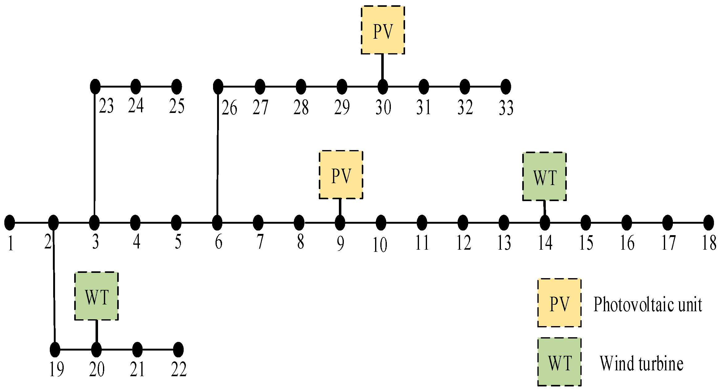
The specific structure of the IEEE 33-bus system is shown in
Figure 3. The base voltage is 12.66 kV and the base capacity is 10 MVA. The photovoltaic systems are connected to nodes 9 and 30, while the wind turbines are connected to nodes 14 and 20. The operating records of a distribution system in a real-world region are used, encompassing hourly load consumption, photovoltaic generation, and wind power output data for 365 days. Time-of-use electricity prices are set with peak periods from 09:00 to 12:00 and 19:00 to 22:00, with a price of 1.09 yuan/(kW·h). The off-peak period is from 00:00 to 08:00, with a price of 0.35 yuan/(kW·h), and the remaining hours are considered off-peak with a price of 0.68 yuan/(kW·h). The shiftable load accounts for 30% of the total load, and the curtailable load accounts for 15%.
5.2. Plan Setup
To verify the effectiveness of the method proposed in this paper, the following four scenarios are set for comparison:
Scenario 1: No demand response considered, bi-level planning of the energy router in a single scenario.
Scenario 2: Demand response considered, bi-level planning of the energy router in a single scenario.
Scenario 3: No demand response considered, bi-level planning of the energy router in multiple scenarios.
Scenario 4: Demand response considered, bi-level planning of the energy router in multiple scenarios.
5.3. Simulation Results
- 1.
Multi-Scenario Clustering
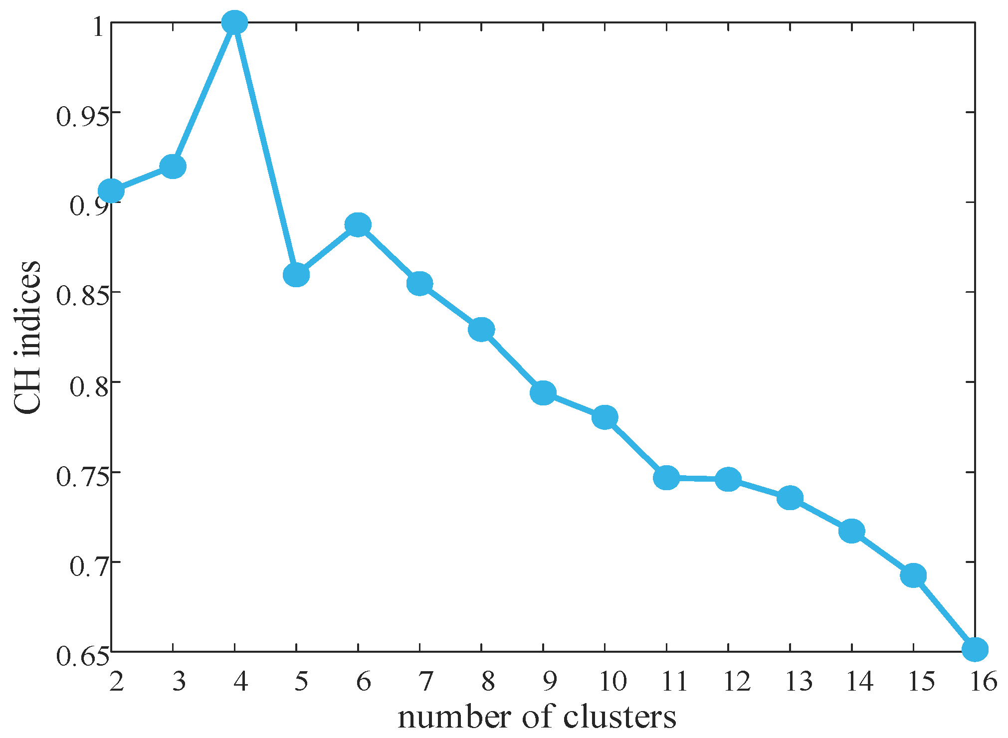
Clustering was performed on the annual output data of photovoltaic (PV) systems, wind turbines, and daily load consumption. The variation in clustering validity indicators for different numbers of clusters is shown in
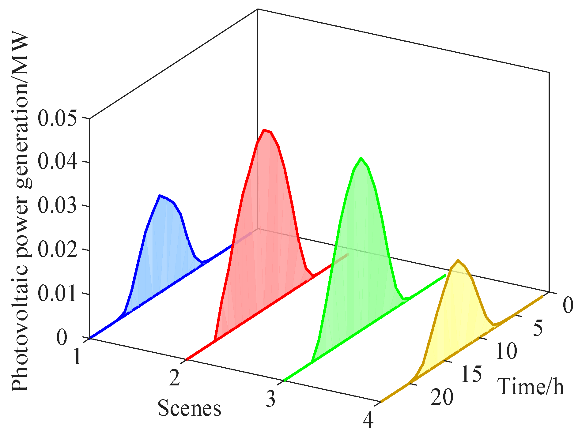
Figure 4. The clustering validity indicator reaches its maximum value when the number of clusters is 4, so the optimal number of clusters is determined to be 4. The probabilities of the four typical scenarios are shown in
Table 1, and the daily output curves of the PV systems, wind turbines, and load for these four typical scenarios are shown in
Figure 5,
Figure 6 and
Figure 7.
- 2.
Bi-Level Planning Results
For different scenarios, the results of energy router location and capacity configuration and the optimized operation of the active distribution network are presented in
Table 2 and
Table 3.
From
Table 2 and
Table 3, it can be seen that when flexible load demand response is considered, the energy storage capacity configuration is larger, indicating that the energy router needs to have sufficient capacity to handle peak demands during load regulation and ensure stable power supply. Furthermore, compared to the single-scenario optimization, the energy storage capacities of Energy Router 1 and Energy Router 2 both increase under the multi-scenario optimization, suggesting that single-scenario optimization cannot meet the diverse load demands. Therefore, in a multi-scenario setting, the energy storage capacity needs to be adjusted to achieve more effective peak shaving and valley filling.
From
Table 3, it is evident that the investment cost of Scenario 1 is lower than that of Scenario 2 and Scenario 3, while Scenario 3 has lower investment costs compared to Scenario 4. This indicates that with the introduction of demand response and multi-scenario optimization, the energy router’s capacity configuration increases, leading to higher investment costs. In terms of operational and maintenance (O&M) costs, Scenario 1 has higher costs than Scenario 2, and Scenario 3 has higher costs than Scenario 4, indicating that the introduction of demand response effectively reduces O&M costs by appropriately adjusting part of the load to avoid peak hours. Regarding security indicators, multi-scenario optimization significantly reduces voltage deviations and network losses, and effectively smooths the load curve through peak shaving and valley filling. This demonstrates that multi-scenario optimization improves the overall system performance. Despite the higher investment costs due to demand response implementation, Scenarios 2 and 4 outperform Scenarios 1 and 3 in terms of voltage deviation improvement and peak shaving and valley filling.
In summary, Scenario 4, benefiting from both demand response and multi-scenario optimization, not only enhances the capacity configuration ability of the energy router but also significantly reduces system operation costs and improves operational efficiency. Therefore, the combination of demand response and multi-scenario optimization significantly optimizes the energy router’s location and capacity decision-making, comprehensively improving the overall performance of the power system.
- 3.
Comparison of Peak Shaving and Valley Filling Effects and Voltage Deviation
To visually compare the optimized operation of the energy router in the active distribution network under different scenarios, a peak shaving and valley filling evaluation index was constructed, as shown in Equation (21):
In the formula,
is the absolute peak-valley difference;
is the peak-valley coefficient;
is the load peak-valley difference rate;
is the optimization rate of peak clipping and valley filling;
is the original absolute peak-valley difference. The peak shaving and valley filling effects for the four scenarios are shown in
Table 4.
From
Table 4, it can be seen that considering flexible load demand response improves the peak shaving and valley filling effects of the active distribution network. Specifically, Scenario 4 outperforms Scenario 3, and Scenario 2 is better than Scenario 1. In particular, the peak shaving and valley filling optimization rate in Scenario 4 is 14.3537%, significantly higher than Scenario 3’s 9.1987%. This indicates that with flexible load demand response, the energy router can respond more flexibly to power fluctuations, balancing the variability of renewable energy, thus improving the grid’s stability and economic efficiency.
Additionally, when comparing Scenario 1 and Scenario 3, although single-scenario optimization is superior in peak shaving and valley filling, multi-scenario optimization makes the energy router’s capacity configuration more adaptable to meet different operational demands under varying load conditions.
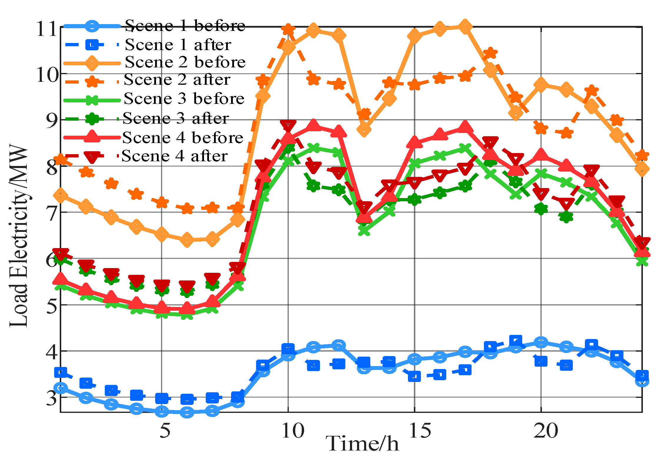
Figure 8 and
Figure 9 illustrate the load curves and voltage deviation behavior before and after multi-scenario optimization with demand response. After multi-scenario optimization and the introduction of demand response, the load curve is significantly smoother, and the peak shaving and valley filling effect is enhanced. In the original case, the load curve exhibits significant fluctuations, especially during high-load periods, leading to increased pressure on power supply. After introducing multi-scenario demand response, the energy router dynamically adjusts the output of the energy storage unit according to load variations across different scenarios, effectively reducing the peaks and filling the valleys, achieving more efficient load regulation.
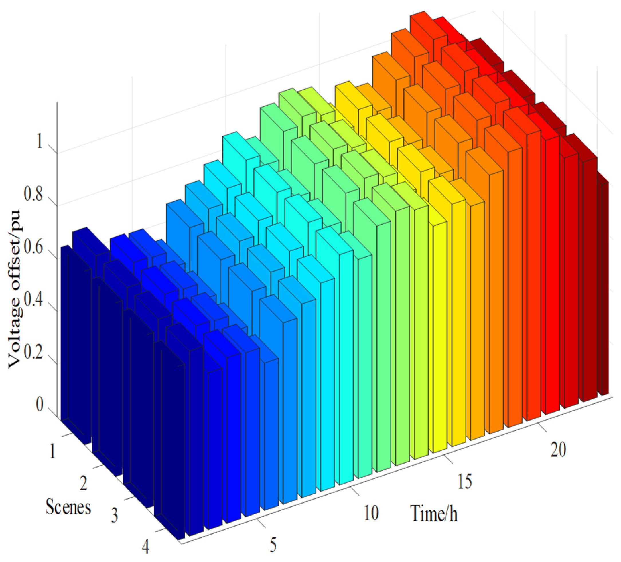
Figure 9 shows the total voltage deviation at each time point in the distribution network after multi-scenario optimization. Under multi-scenario optimization, the energy router coordinates the dispatch of energy storage and renewable energy, maintaining a small and stable voltage deviation from 1 to 12 h, ensuring voltage stability. Although voltage deviation increases between 13 and 24 h due to higher load demands and renewable energy fluctuations, the collaboration between multi-scenario optimization and demand response significantly reduces voltage fluctuations. The energy router can adjust the energy storage and renewable energy outputs in real time to prevent excessive voltage deviation, ensuring stable grid operation during high-load periods.
5.4. Sensitivity Analysis of Flexible Load Ratio
To further assess the impact of flexible load participation on the energy router configuration strategy and system operating performance, a sensitivity analysis is conducted on the participation ratio of flexible loads. Building upon Scenario 4 as a baseline, the proportions of shiftable load and curtailable load within the total load are varied to examine their effects on key indicators such as siting and sizing schemes, system comprehensive cost, voltage deviation, and power fluctuation.
In the default setting, the flexible load ratio is defined as 30% for shiftable load and 15% for curtailable load. Based on this, the following four comparative scenarios are established:
Scenario 1: Shiftable load accounts for 10% of the flexible load, and curtailable load accounts for 5%.
Scenario 2: Shiftable load accounts for 20% of the flexible load, and curtailable load accounts for 10%.
Scenario 3: Shiftable load accounts for 30% of the flexible load, and curtailable load accounts for 15%.
Scenario 4: Shiftable load accounts for 40% of the flexible load, and curtailable load accounts for 20%.
A two-layer optimization for ER siting and sizing is performed under different flexible load ratios, and the resulting configuration is shown in
Table 5. As the flexible load participation ratio increases, the ER siting and capacity configuration exhibit some degree of adjustment. With the support of a high-ratio response capability, the system’s dependence on energy storage resources decreases, causing the ER configuration capacity to show a decreasing trend. This change indicates that enhanced load regulation capabilities can, to some extent, replace the physical support of energy storage facilities, thereby effectively reducing system investment requirements and configuration costs. Simultaneously, the improvement in the flexible load level also affects the selection of the optimal access node for the ER, reflecting its feedback effect on the system’s operating state and further validating the necessity of collaborative optimization of multi-source loads in practical applications.
From the perspective of operating performance, as shown in
Table 6, the improvement of the flexible load ratio significantly improves the overall operating performance of the system. Specifically, the comprehensive cost gradually decreases from Scenario 1 to Scenario 4, with a cumulative decrease of approximately 4.4%. Although the response incentive cost increases, the investment and operation and maintenance costs decrease simultaneously, reflecting the cost advantage of load-side regulation in alleviating system operating pressure. Furthermore, the magnitude of power fluctuation decreases significantly, indicating that the system load curve tends to be smoother, and peak shaving and valley filling capabilities are significantly enhanced. The voltage deviation and network loss indicators also improve accordingly, further verifying the role of flexible loads in improving power quality and system stability.
In summary, as the flexible load participation ratio increases, the flexibility, economic efficiency, and security of system operation are all enhanced, fully illustrating the positive significance of introducing demand response mechanisms in active distribution networks for the optimized configuration of energy routers and system operation scheduling.
5.5. Comparison of Different Solution Algorithms
To evaluate the optimization performance of the improved bi-level particle swarm optimization (PSO) algorithm, this paper compares it with the traditional bi-level PSO and simulated annealing-particle swarm hybrid optimization algorithm. The population size for both upper and lower layers is set to 50, with 30 iterations for the lower layer. For each iteration of the upper layer, the lower layer performs 30 iterations. All algorithms were independently executed 30 times on the MATLAB 2023a platform, and the results are shown in
Table 7, with iteration curves depicted in
Figure 10.
The results indicate that the improved bi-level PSO algorithm reduces the number of iterations and convergence time by 44.4% and 42.1%, respectively, compared to the traditional bi-level PSO. In comparison with the simulated annealing-particle swarm hybrid optimization algorithm, the reductions are 33.3% and 15.3%, respectively. Furthermore, the improved algorithm achieves better performance in terms of the optimal objective function value, demonstrating that the multi-strategy fusion mechanism significantly enhances the optimization efficiency and solution accuracy of the bi-level PSO algorithm.


 ,
, 


