Dynamic Scheduling for Multi-Objective Flexible Job Shops with Machine Breakdown by Deep Reinforcement Learning

Abstract

Dynamic scheduling for flexible job shops under machine breakdown is a complex and challenging problem due to its valuable application in real-life productions. However, prior studies have struggled to perform well in changeable scenarios. To address this challenge, this paper introduces a dual-objective deep reinforcement learning (DRL) to solve this problem. This algorithm is based on the Double Deep Q-network (DDQN) and incorporates the attention mechanism. It decouples action relationships in the action space to reduce problem dimensionality and introduces an adaptive weighting method in agent decision-making to obtain high-quality Pareto front solutions. The algorithm is evaluated on a set of benchmark instances and compared with state-of-the-art algorithms. The experimental results show that the proposed algorithm outperforms the state-of-the-art algorithms regarding machine offset and total tardiness, demonstrating more excellent stability and higher-quality solutions. At the same time, the actual use of the algorithm is verified using cases from real enterprises, and the results are still better than those of the multi-objective meta-heuristic algorithm.

1. Introduction

The flexible job shop is a common production scheduling environment characterized by its ability to accommodate customized manufacturing requirements. The production landscapes encompassing semiconductor manufacturing processes, building materials manufacturing, and mechanical manufacturing systems can be abstractly distilled into the realm of flexible job shop scheduling problems. Recognized as a non-deterministic polynomial-hard (NP-hard) problem [1], each operation can be assigned to a different machine, and the processing time on each machine is not necessarily the same; the flexible job shop scheduling problem (FJSP) has garnered extensive utilization within modern industries. Its intricate nature and profound interconnection with the production environment have spurred comprehensive investigations into FJSP modeling and solution methodologies [2]. Compared to traditional job shop scheduling, the FJSP presents greater complexity in machine selection and operation sequencing, requiring more efficient real-time rescheduling strategies when facing dynamic disruptions [3]. Therefore, this paper investigates the dynamic flexible job shop scheduling problem (DFJSP) under machine breakdown scenarios, and a reinforcement learning algorithm for solving this complex problem is proposed.

In previous studies, solving FJSPs in ideal static environments has developed into a well-established framework, focusing on achieving global optimal resource allocation through mathematical modeling and algorithm design. Mathematical programming, heuristic algorithms, and meta-heuristic algorithms, such as improved genetic algorithms and hybrid particle swarm optimization, continue to advance in theoretical optimization and computational efficiency. However, the dynamic nature of real-world production environments, characterized by machine breakdowns, job arrivals, and job cancellations, poses significant challenges to traditional scheduling methods. For instance, Yao et al. [4] proposed a mixed integer linear programming (MILP) model based on the modified disjunctive graph, which can obtain the optimal solutions for benchmark instances. Creating an MILP model is helpful for addressing the shop scheduling problem. Shi and Xiong [5] developed an enhanced NSGA-II algorithm, and results show that the algorithm outperforms the other algorithms in solving the problem of job shop scheduling. Existing static scheduling models typically rely on deterministic production environments and fixed parameter assumptions. As a result, they are often ineffective in solving dynamic disruptions commonly encountered in real manufacturing systems. These disruptions can include unexpected machine breakdowns, urgent job insertions, and job reprocessing due to quality issues [6]. This disconnect between theory and practice significantly reduces the robustness and adaptability of traditional scheduling methods in dynamic environments. Empirical studies by Tariq et al. [7] indicate that dynamic disturbances in job shop scheduling can significantly impact the initial scheduling plan, particularly if the machine breakdown, leading to the plan’s complete failure to execute. Developing an algorithm that can respond quickly to dynamic disturbances is essential. Studies have shown that, given the increasing demand for customized products, problem sizes grow, job and machine coupling constraints become overly complex, and the optimality guarantee rate of traditional static scheduling algorithms drops sharply [8,9].

This highlights the gap between static scheduling theory and the dynamic, complex demands of industrial applications, providing a practical impetus for research in dynamic scheduling. To this end, research on dynamic flexible job shop scheduling has emerged as a frontier in intelligent manufacturing. By incorporating real-time data acquisition technologies such as digital twins and Internet of Things (IoT) sensing, scholars have developed hybrid response mechanisms based on event-driven and periodic-driven strategies, providing a foundation for data collection in dynamic scheduling studies [10].

As a core challenge in optimizing complex manufacturing systems, dynamic scheduling has long been a focal point in operations research and industrial engineering. Heuristic and metaheuristic algorithms are commonly used to address this complex problem [11]. Research in heuristic algorithms primarily focuses on dispatch rules designed for specific problem characteristics. In contrast, metaheuristic algorithms employ swarm intelligence search mechanisms to explore global optimal solutions, such as genetic algorithms (GAs), differential evolution (DE), Tabu search (TS) and particle swarm optimization (PSO). Yao et al. [12] propose a knowledge-based multi-objective evolutionary algorithm to simultaneously optimize makespan and total energy consumption, with a particular focus on the energy impact of mobile robots. Sun et al. [13] proposed a hybrid non-dominated sorting genetic algorithm with Tabu search to optimize the multiple objectives simultaneously. Xie et al. [14] proposed a hybrid genetic Tabu search algorithm to optimize distributed flexible job shop scheduling. The algorithm aims to minimize the makespan, demonstrating superior performance in the benchmark instances. Burmeister et al. [15] proposed a multi-objective memetic algorithm based on the non-dominated sorting genetic algorithm with both makespan and energy cost minimization as the objectives, evaluating the approach by conducting computational experiments using prominent benchmark instances and presenting the better solutions on the approximated Pareto front. In the research by Zhang et al. [16], a genetic programming approach is proposed for dynamic FJSPs. The algorithm integrates dispatch rule size considerations via multitask learning with knowledge sharing into scheduling algorithms, having a good balance between exploration and exploitation during the evolutionary process.

Metaheuristic algorithms always divide the dynamic scheduling problem into a series of static sub-problems and then use the optimization algorithms to solve these sub-problems separately. Although this approach can yield high-quality solutions, its computational cost makes it unsuitable for real-time dynamic scheduling. As a result, an increasing number of researchers are using deep reinforcement learning to solve complex dynamic problems. Gui et al. [17] proposed an optimization algorithm based on DRL to solve the FJSP with job insertion. Research demonstrates that this method greatly enhances scheduling performance in dynamic scheduling at the generated random data set and can effectively select the appropriate scheduling rules at the time of scheduling. Hammami et al. [18] applied a DRL-based approach to solving the real-time job shop scheduling problem faced with unexpected job arrivals. The results indicate that for small batches of incoming jobs, the problem can be solved in real time with a better solution. Zhao et al. [19] proposed a DRL-based reactive scheduling approach using proximal policy optimization with an attention policy network designed to enable real-time decision-making for random job arrivals. Experimental results demonstrate that the proposed method performs better across various production configurations and is more effective for dynamic scheduling needs in real manufacturing scenarios. Gan et al. [20] used deep reinforcement learning to solve the machine breakdown problem in the job shop. The proposed scheduling scheme is highly robust and stable, and has a shorter running time than the traditional algorithm.

Current research primarily focuses on using meta-heuristic algorithms to solve various types of job shop scheduling problems, including FJSP. The application of deep reinforcement learning to FJSP under machine breakdown remains in its early stages. Meta-heuristic algorithms are suitable for solving static scheduling problems, but these methods struggled to meet the instant response requirements of dynamic scheduling. Traditional Double Deep Q-network (DDQN) also faces challenges in learning two conflicting objectives, with previous studies often merging them into a single objective. Therefore, the main of this research is to develop an optimization algorithm based on deep reinforcement learning to efficiently and accurately select the most appropriate dispatch rules at each scheduling moment, thereby achieving a balance between timeliness, scheduling performance, and objectives. Additionally, the advantages of DRL over traditional metaheuristic algorithms in terms of solution quality and generalization have yet to be clearly demonstrated. This paper proposes a novel framework to address the interplay between these optimization objectives. The contributions of this work are summarized as follows.

• Problem Characteristics: Machine breakdown is a common occurrence in a wide range of discrete machining and manufacturing environments, such as the processing and manufacturing of aviation, aerospace, ships, and parts. In this paper, DFJSP with random machine breakdown is considered. The optimization objectives are set as the total tardiness of jobs and machine offset, which are most susceptible to machine breakdown in natural production.
• Algorithm Characteristics: An improved Double Deep Q-network for dual-objective (IDDQN-II) DFJSP is proposed based on the DDQN framework. The hierarchical algorithm IDDQN-II cleverly decomposes the optimization difficulty of the dual objectives and decouples the selection of jobs and machines, realizing more combined dispatch rules to deal with different scheduling environments.
• Experiment results: In the experiment section, the IDDQN-II is compared with widely used multi-objective meta-heuristic algorithms on the benchmark. Additionally, the case derived from actual enterprises is introduced to validate the algorithm. The IDDQN-II algorithm has achieved excellent results and has been verified for effectiveness.

The remaining sections of this paper are organized as follows. The problem details and the mathematical model of DFJSP are introduced in Section 2. A detailed presentation of our algorithm design is provided in Section 3. A prospective experimental comparison is conducted, and the results are comprehensively analyzed in Section 4. Finally, Section 5 concludes this paper.

2. Problem Description and Mathematical Model

2.1. Problem Description

The dual-objective dynamic flexible job shop rescheduling problem under machine breakdown, considering machine offset and total job tardiness, can be described as follows: The job shop consists of $M=\{M_1,M_2,\dots ,M_k\}$ machines and $J=\{J_1,J_2,\dots ,J_i\}$ of jobs to be processed. Each job $J_i$ consists of $n_i$ sequential operations, while each operation has $M_{i,j}$ machines available for processing, and all jobs have delivery time constraints. The deadline of the job $J_i$ is defined as $J_i$, and the machine offset is R. When rescheduling occurs, it is constrained by the machine offset optimization objective. This research aims to minimize the total tardiness of all jobs and machine offset while reducing the impact of dynamic events on job shop scheduling and responding promptly to disruptions caused by machine breakdown.

When machine M breaks down while processing operation $O_{i,j}$ at time t, rescheduling is required in two scenarios: (1) the breakdown machine is actively processing, or (2) the breakdown machine is idle but has pending tasks awaiting allocation. In the natural production environment, the rescheduling result leaves completed jobs unaffected, while operations on breakdown machines are immediately interrupted and require reprocessing. Meanwhile, operations being processed on functioning machines continue as planned, though subsequent scheduling may be adjusted. The following assumptions are made to facilitate the research of the DFJSP problem.

(1)

The transportation time of jobs between machines is empty.

(2)

The delivery time of jobs remains unchanged even if their assigned machines change, and after rescheduling, the processing time $P_{i,j,k}$ is independent of the machine’s current load status.

(3)

The processing time for each operation on available machines is known.

(4)

It is assumed that one machine breaks at the same time.

2.2. Mathematical Model

An MILP model is established to accurately describe the DFJSP. In this context, the dual objectives are to minimize total tardiness and machine offset. Based on the notation in Table 1, the DFJSP discussed in this paper can be mathematically formulated as follows.

Table 1. Notations description.

Notations	Description
$i,h$	The index of job
$j,g$	The index of operation
n	Total number of jobs
m	Total number of machines
$J_i$	i-th job
$n_i$	The number of operations for $J_i$
$M_k$	k-th machine
$M_{i,j}$	The available machine set $M_1,\dots M_k$ for the $O_{i,j}$
$O_{i,j}$	The j-th operation of $J_i$
$S_{i,j}$	The start processing time of operation $O_{i,j}$
$C_{i,j}$	The completion time of operation $O_{i,j}$
$C_i$	The completion time of $J_i$
$P_{i,j,k}$	The processing time of operation $O_{i,j}$ on machine $M_k$
$D_i$	The due date of $J_i$
$X_{i,j,k}$	If operation $O_{i,j}$ is processed on $M_k$, $X_{i,j,k}$ = 1; else $X_{i,j,k}$ = 0
$N_{i,j,h,g}$	If $O_{h,g}$ is the previous operation adjacent to $O_{i,j}$, $N_{i,j,h,g}$ = 1; If $O_{h,g}$ is the next operation adjacent to $O_{i,j}$, $N_{i,j,h,g}=-1$; else $N_{i,j,h,g}$ = 0
t	Scheduling time
$M_k\left(t\right)$	Machine status at time t, if the machine breakdown $M_k\left(t\right)=-1$, else $M_k\left(t\right)$ = 1

The total tardiness of jobs reflects the timeliness of order delivery, directly impacting customer satisfaction and supply chain stability. The objective aims to maximize on-time delivery across all jobs, thereby reducing inventory and management costs while minimizing additional expenses caused by delivery delays. The total tardiness objective D can be described as follows.

$$minD=\sum _{i=1}^{n}max\left(C_i-D_i,0\right)$$

(1)

Machine offset is commonly used to quantitatively assess the discrepancies between rescheduling and the original scheduling plan caused by dynamic events. Machine offset is defined as the changes for processing operations after rescheduling compared to the original schedule in this paper. Significant fluctuations in machine offset can lead to instability in machine load and processing parameters, increasing equipment wear, abnormal energy consumption, and risks to process quality. Minimizing machine offset helps mitigate these issues while preventing material preparation disruptions and reducing resource wastage. The machine offset objective R can be described as follows.

$$minR=\sum _{i=1}^n\sum _{j=1}^{n_i}\mathbb{I}(k_{i,j}^t\ne k_{i,j}^0)$$

(2)

Since each operation can be processed on multiple candidate machines, the initial machine assignment for operation $O_{i,j}$ is defined as $k_0^{i,j}$. If the operation is reassigned to a different machine $k_t^{i,j}$ during rescheduling at time t, a machine offset counter is triggered. The indicator function $\mathbb{I}\left(\right)$, a specialized function for conditional evaluation, is typically defined as Equation (3).

$$\mathbb{I}\left(condition\right)=\left\{\begin{array}{cc}1,\hfill & Conditionsatisfied\hfill \\ 0,\hfill & Conditionunsatisfied\hfill \end{array}\right.$$

(3)

Among them, $C_i$ is the last operation completion time of $J_i$.

$$C_i=C_{i,n_i},\forall i\in \{1,2,\cdots ,n\}$$

(4)

And the completion time of operation $O_{i,j}$ can be calculated as

$$\begin{array}{c}\hfill C_{i,j}=S_{i,j}+\sum _{k=1}^m{P}_{i,j,k}\times X_{i,j,k},\forall i\in \{1,2,\cdots ,n\},j\in \{1,2,\cdots ,n_i\}\end{array}$$

(5)

Each operation can only be executed on one machine at the same time can be described as

$$\begin{array}{c}\hfill \sum _{k\in M_{i,j}}{X}_{i,j,k}=1,\forall i\in \{1,2,\cdots ,n\},j\in \{1,2,\cdots ,n_i\}\end{array}$$

(6)

The process sequence constraint can be described as

$$\begin{array}{c}\hfill S_{i,j}-C_{i,j-1}>0,\forall i\in \{1,2,\cdots ,n\},j\in \{1,2,\cdots ,n_i\}\end{array}$$

(7)

The operation can only be processed on normal machines. This can be described as

$$\begin{array}{cc}\hfill & X_{i,j,k}{M}_k\left(t\right)\ge 0,\forall i\in \{1,2,\cdots ,n\},j\in \{1,2,\cdots ,n_i\},k\in \{1,2,\cdots ,m\},0\le t\le max\left(C_i\right)\hfill \end{array}$$

(8)

Each machine processes only one operation at a time sequentially.

$$\begin{array}{cc}\hfill & (S_{h,g}-C_{i,j})X_{i,j,k}{X}_{h,g,k}(N_{i,j,h,g}+1)+(S_{i,j}-C_{h,g})X_{i,j,k}{X}_{h,g,k}(1-N_{i,j,h,g})\ge 0,\hfill \\ \hfill & \forall i,h\in \{1,2,\cdots ,n\},j,g\in \{1,2,\cdots ,n_i\},k\in \{1,2,\cdots ,m\}\hfill \end{array}$$

(9)

The breakdown time t for machine follows a Weibull distribution [21]. Considering the impact of aging on machines, the probability of machine breakdown is directly associated with time. For this paper, specific values are chosen for the shape parameter k and the scale parameter $\lambda$ set at 5 and 1, respectively, aligning with the distinctive characteristics of the DFJSP.

$$M{S}_k\left(t\right)=\left\{\begin{array}{cc}{\displaystyle \frac{k}{\lambda }}{\left({\displaystyle \frac{t}{\lambda }}\right)}^{k-1}{e}^{-{\left({\displaystyle \frac{t}{\lambda }}\right)}^k},\hfill & t\ge 0;\hfill \\ 0,\hfill & t<0.\hfill \end{array}\right.$$

(10)

Optimizing total tardiness alone may lead to frequent machine load fluctuations and deteriorating conditions, while overly restricting machine offset may result in infeasible schedules that fail to satisfy delivery requirements. This research considers a dual-objective optimization problem for DFJSP based on deep reinforcement learning to address this.

3. Algorithm Design

Deep reinforcement learning faces significant challenges when optimizing multiple interrelated or conflicting objectives simultaneously. Effectively capturing the dynamic balance between these objectives in the reward function is difficult, as the importance of each objective can vary nonlinearly based on the environmental state or specific task requirements. Traditionally, deep reinforcement learning algorithms have relied on reward feedback mechanisms [22]. However, in multi-objective scenarios, rewards, goal coupling, and non-stationarity conflicts can cause issues such as forgetting objectives and deviations in convergence during agent training [23]. Additionally, the combination of high-dimensional state spaces and multi-objective decision spaces further increases the complexity of policy exploration. Moreover, dynamically balancing the priorities of different objectives during the learning process to prevent neglect or excessive optimization remains a critical challenge. To effectively solve the dual-objective optimization problem in flexible job shop rescheduling, this paper builds on the core framework of DDQN and proposes a hierarchical DRL approach.

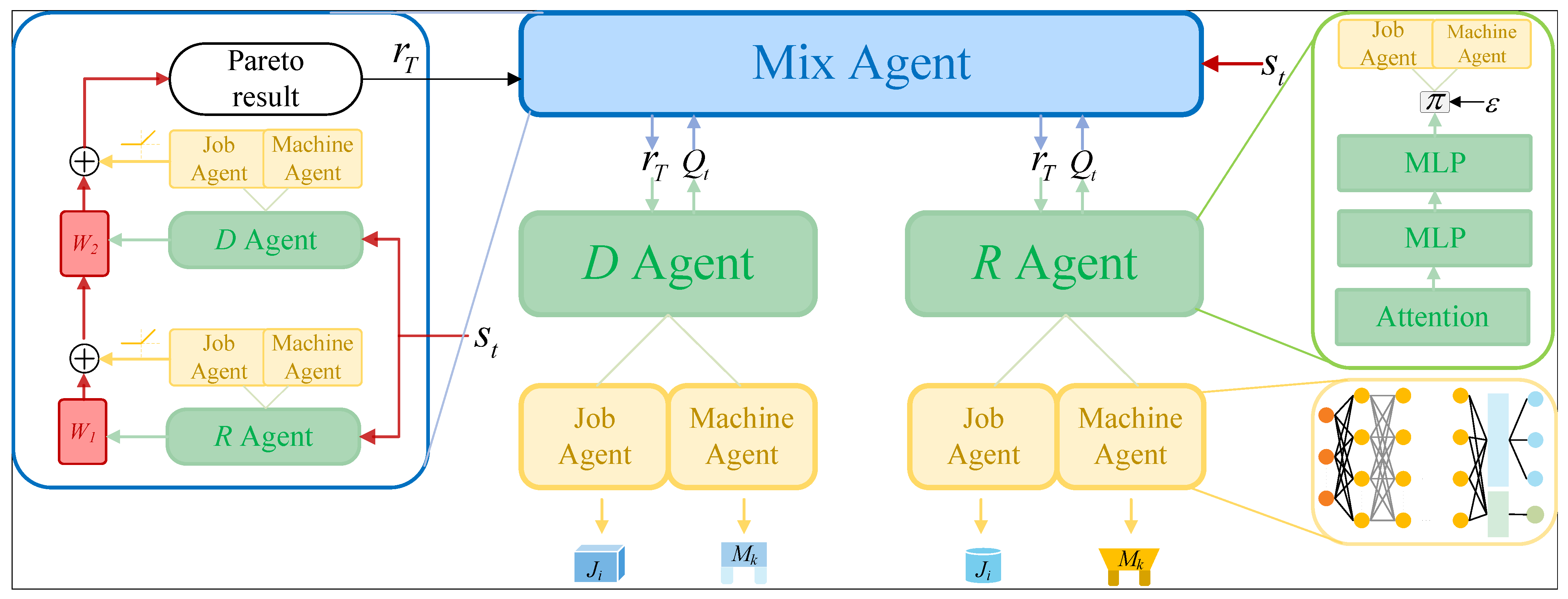
In dynamic scenario optimization based on deep reinforcement learning, conventional DQN often suffers from policy oscillations due to value estimation bias [24], and their single-objective optimization struggles to satisfy the multiple demands of complex natural industrial environments. This paper presents a hierarchical framework of an Improved Double Deep Q-network (IDDQN-II) that integrates dual-objective optimization to tackle these challenges. The proposed algorithm reduces overall job tardiness and machine offset by creating a decoupled value evaluation agent and a structured decision-making process. The framework of IDDQN-II is depicted in Figure 1. The core of the algorithm is centrally located in the figure, and a hierarchical framework assigns various algorithm layers to different functions. Simultaneously, each layer’s working agent mode is displayed in the same-colored boxes. Each layer must work together to output a complete solution, but they are independent at runtime. The layer combines each lower layer to achieve its own function, and each lower layer feeds back to the upper layer in competition.

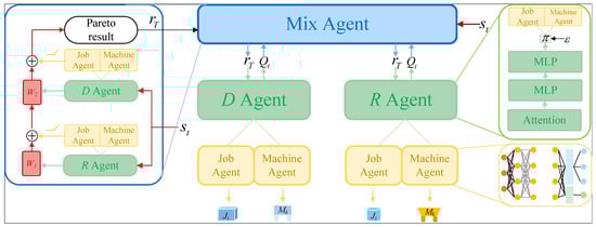
Figure 1. The framework of IDDQN-II.

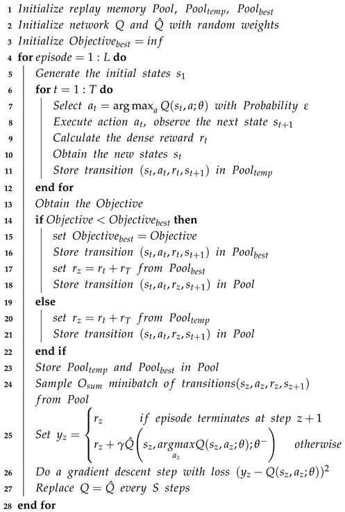
In this framework, two agents are independently trained to optimize total job tardiness and minimize machine offset, following the process outlined in Algorithm 1. This independent training approach effectively decouples the optimization objectives, improving solution quality. Unlike some DRL methods that rely on weighted-sum approaches, which often limit the exploration of the solution space in multi-objective optimization, this method ensures a more comprehensive search. The output of the agent consists of two sub-agents that categorize different agents into groups for job and machine selection. By separating these two processes in the action space, the dispatch rules for job and machine selection can be decoupled. This approach offers more flexible combinations of dispatch rules and allows for a more comprehensive exploration of the solution space. While the training phase focuses on disentangling complex optimization relationships, an adaptive weighting strategy is employed at the top-level mixed agent during the result to generate high-quality Pareto-optimal solutions.

Algorithm 1: The training process detail of Agent

3.1. State Features

In deep reinforcement learning, state features are crucial inputs that enable the agent to understand its environment and make informed decisions. Designing effective state features is essential for addressing complex scheduling problems, as these features must accurately represent dynamic factors such as machine workload, process progression, and competition for resources. A good state representation should provide a complete environmental description, adapt in real time, be sensitive to multi-objective interactions, and be suitable with the DRL framework. This paper proposes a hierarchical IDDQN-II framework, where agents at different layers address distinct objectives. Each agent requires tailored state inputs to represent past scheduling events and environmental changes, enabling optimal decision-making based on the current state. Before delving into the state feature, this research needs to define the following parameters: $T{M}_k\left(t\right)$ is the completion time of the last process on machine $M_k$ at time t, and $T_c$ is the average completion time of all machines. $O{J}_i\left(t\right)$ is the number of operations of $J_i$ has completed at time t. $R_k\left(t\right)$ is the completion rate of the job of $J_i$ at time t.

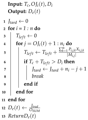
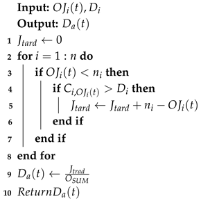
The input state of the agent, optimized for minimizing the total tardiness D, includes the number of jobs n, the number of machines m, the average processing wait rate of job operations $TR{J}_i\left(t\right)={\displaystyle \frac{{\sum }_{i=1}^n{\sum }_{j=1}^{O{J}_i\left(t\right)}{\sum }_{\dot{k}}{P}_{i,j,k}}{{\sum }_{i=1}^{n}max\left(C_i\right)}}$, the average job completion rate $F{J}_i\left(t\right)={\displaystyle \frac{1}{n}}{\sum }_{i=1}^n{\displaystyle \frac{O{J}_i\left(t\right)}{n_i}}$ and its standard deviation, the average machine utilization rate $R_{ave}\left(t\right)={\displaystyle \frac{{\sum }_{k=1}^m{R}_k\left(t\right)}{m}}$ and its standard deviation, the average machine flexibility rate $M_{k}P\left(t\right)={\displaystyle \frac{{\sum }_{k=1}^m{\sum }_{i=1}^n{\sum }_{j=O{J}_i\left(t\right)}^n{O}_{i,j}{X}_{i,j,k}}{{({\sum }_{i=1}^n{n}_i-{\sum }_{i=1}^{n}O{J}_i\left(t\right))}^{\ast }m}}$ and its standard deviation, the estimated job tardiness rate $D_e\left(t\right)$ as shown in Algorithm 2, and the actual job tardiness $D_a\left(t\right)$, as shown in Algorithm 3.

Algorithm 2: $D_e\left(t\right)$

Algorithm 3: $D_a\left(t\right)$

The input state for the agent optimizing machine deviation includes the number of jobs n, the number of machines m, the average waiting rate of job operations $TR{J}_i\left(t\right)$, the average completion rate of jobs $F{J}_i\left(t\right)$ and its standard deviation, the average machine utilization $R_{ave}\left(t\right)$ and its standard deviation, the average machine flexibility $M_{k}P\left(t\right)$ and its standard deviation, the machine offset rate $M_{k}D\left(t\right)$, and the Gini coefficient of shop machine workload $G_k\left(t\right)$. The Gini coefficient [25], originally a widely used metric in economics, quantifies the degree of inequality in a given parameter or system. It ranges from 0 to 1, where 0 indicates perfect equality, and 1 represents extreme inequality. In this study, the Gini coefficient is introduced as a measure of machine load balance. It is defined as twice the area between the Lorenz curve and the line of absolute equality(diagonal). Assuming there are m machines in the workshop, the current machine load ratio set is defined as $U=\{U_1,U_2,\cdots ,U_m\}$. The horizontal axis represents the cumulative proportion of machines (ranging from 0% to 100%), while the vertical axis denotes the cumulative load proportion (ranging from 0% to 100%). $G_k\left(t\right)$ is computed using Equation (11).

$$G_k\left(t\right)={\displaystyle \frac{{\sum }_{x=1}^m{\sum }_{z=1}^m|U_x-U_z|}{2m^2{R}_{ave}\left(t\right)}}$$

(11)

The machine deviation rate $M_{k}D\left(t\right)$ can be calculated by Equation (12), where $O_{init}$ represents the number of operations processed before machine breakdown.

$$M_{k}D\left(t\right)={\displaystyle \frac{{\sum }_{j=1}^{O_{sum}}\mathbb{I}(k_j^t\ne k_j^0)}{O_{sum}-O_{init}}}$$

(12)

The input state of the job–agent consists of job-related features: the average waiting rate of job operations $T{R}_{Ji}\left(t\right)$, the average completion rate $F_{Ji}\left(t\right)$ and its standard deviation. Additionally, it incorporates optimization objectives from higher-level agents, including the estimated tardiness rate $D_e\left(t\right)$, actual tardiness $D_a\left(t\right)$, or machine offset rate $M_{k}D\left(t\right)$, as well as the Gini coefficient of shop machine workload $G_k\left(t\right)$. The input state of the machine–agent, which is responsible for machine selection, focuses solely on state features related to machines. These include the average machine utilization $R_{ave}\left(t\right)$ and its standard deviation, the average machine flexibility $M_{k}P\left(t\right)$ and its standard deviation, as well as the optimization objectives considered by the higher-level agent, such as the estimated tardiness rate $D_e\left(t\right)$, actual tardiness $D_a\left(t\right)$, or machine deviation rate $M_{k}D\left(t\right)$, and the shop floor load Gini coefficient $G_k\left(t\right)$. The hierarchical design has clearly expanded the state dimensions. The attention mechanism [26] is explicitly incorporated into this paper’s neural network architecture design to address this. The self-attention mechanism captures the dynamic temporal dependencies and resource competition patterns between operations, providing the deep reinforcement learning model with crucial environmental awareness. This module employs multi-head parallel computation to extract potential correlations from multi-dimensional state features, such as the number of jobs n, the number of machines m, the average waiting rate for job operations $TR{J}_i\left(t\right)$, the average completion rate $F{J}_i\left(t\right)$ and its standard deviation, the average machine utilization rate $R_{ave}\left(t\right)$ and its standard deviation, the average machine flexibility rate $M_{k}P\left(t\right)$ and its standard deviation, the machine offset rate $M_{k}D\left(t\right)$, and the job shop load Gini coefficient $G_k\left(t\right)$. It utilizes residual connections and layer normalization to maintain gradient stability, enabling the agent to adaptive focus on key scheduling time. This allows precise coordination of machine allocation and operation sequencing strategies under dynamic disturbances, such as machine breakdown, effectively supporting the dual-objective collaborative optimization of minimizing machine offsets and total tardiness. The inherent global information interaction significantly enhances the agent’s ability to analyze complex production coupling relationships, providing a foundation for adaptive weight adjustment and dynamic decision-making through high-dimensional feature representation.

3.2. Action Space

The action space of the agent is designed to enable the selection of dispatch rules for job and machine allocation. The job–agent selects the optimal job scheduling rule from a set of candidate rules, while the machine–agent selects the best machine allocation rule. In previous research on FJSPs, the flexibility of machines has often been overlooked, yet it remains a key factor that constrains scheduling quality. Decouple the dispatch rules for job and machine selection and provide a more flexible combination of dispatch rules that allows the agent to explore the solution space more thoroughly. Different rules should be applied based on the various production statuses. Consequently, the dispatch rules are used as an action space for the agent’s output. The selection of machines and jobs is based on concepts from previous research and the characteristics of the problem, and previous experiments have confirmed the effectiveness of these dispatch rules [27,28,29]. The job–agent has seven actions, which are as follows:

(1)

Select the job with the most remaining operations at the current time.

(2)

Select the job with the lowest processing rate at the current time.

(3)

Select the job with the shortest time to tardiness at the current time.

(4)

Select the job with the largest estimated tardiness at the current time.

(5)

Select the job with the longest remaining processing time at the current time.

(6)

Select the job with the shortest remaining processing time at the current time.

(7)

Select the job that can be processed the earliest at the current time.

The machine agent has three actions, which are as follows:

(1)

Select the machine with the lowest load rate at the current time.

(2)

Select the machine with the worst processing capability at the current time.

(3)

Select the machine that can start processing the earliest at the current time.

After decoupling the selection of jobs and machines, the upper-level agent independently chooses to prioritize jobs or machines. This allows for a more significant number of combined dispatch rules through permutation and combination. More importantly, the action space is smaller for the sub-agent, which means the range the sub-agent needs to explore is reduced, thereby lowering the training difficulty. The neural network structures of the two sub-agents are shown in Figure 2. The neural network structures used in this paper consist of five fully connected layers, which are composed of one input layer, one output layer and three hidden layers. The number of nodes in the input and output layers corresponds to the number of state features and available actions. In this paper, the “ReLU” activation function is utilized for the input and hidden layers, while the “Purelin” activation function is used for the output layer.

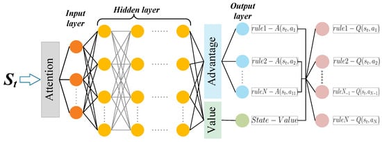
Figure 2. The structures of agent.

3.3. Reward Function

In this paper, the reward is composed of two parts: the dense reward $r_t$ and the sparse reward $r_T$. Dense reward help the agent recognize the job shop environment at different time steps, while sparse reward enables the agent to learn the contribution of each action to the scheduling result and optimization objective. After the top-level agent obtains the scheduling solution, it converts this into $r_T$ and transmits it to the lower-level agents. The optimization objective for the agent responsible for minimizing the total tardiness of the jobs, and its sub-agents, is defined as $r_T$ for the experience stored in the memory pool: $r_T=(D_{Best}-D)/O_{sum}$, and for other experiences in the best memory pool: $r_T=(D-D_{Best})/O_{sum}$. For the agent responsible for the machine offset, and its sub-agents, the optimization objective is defined as $r_T$ for the experience in the memory pool: $r_T=(R_{Best}-R)/O_{sum}$, and for other experiences in the best memory pool: $r_T=(R-R_{Best})/O_{sum}$.

The optimization objective for the agent with machine offsets, where the lower-level job–agent is responsible for job selection, can be calculated using the dense reward $r_t$ as described in Algorithm 4.

Algorithm 4: Dense reward $r_t$

$Deflection\leftarrow \left({\displaystyle \frac{M_{k}D\left(t\right)}{M_{k}D(t+1)}}\right)M_{k}D\left(t\right)+\left({\displaystyle \frac{G_k\left(t\right)}{G_k(t+1)}}\right)G_k\left(t\right)$ $Affect\leftarrow \left({\displaystyle \frac{TR{J}_i(t+1)}{TR{J}_i\left(t\right)}}\right)TR{J}_i\left(t\right)+\left({\displaystyle \frac{F{J}_i(t+1)}{F{J}_i\left(t\right)}}\right)F{J}_i\left(t\right)$ $r_t\leftarrow Affect-Deflection$ $Return{r}_t$

Similarly, the dense reward $r_t$ for the machine–agent responsible for machine selection in the optimization target for machine offset can be calculated using Algorithm 5. The upper-level agent’s $r_t$ is the cumulative reward obtained by the two lower-level sub-agents. For the optimization target aiming to minimize total job tardiness, the reward $r_t$ for the lower-level sub-agents is calculated similarly, with the only modification being the change in parameters in $Deflection$ to $D_e\left(t\right)$ and $D_a\left(t\right)$.   

Algorithm 5: Dense reward $r_t$

$Deflection\leftarrow \left({\displaystyle \frac{M_{k}D\left(t\right)}{M_{k}D(t+1)}}\right)M_{k}D\left(t\right)+\left({\displaystyle \frac{G_k\left(t\right)}{G_k(t+1)}}\right)G_k\left(t\right)$ $Affect\leftarrow \left({\displaystyle \frac{R_{ave}(t+1)}{R_{ave}\left(t\right)}}\right)R_{ave}\left(t\right)+\left({\displaystyle \frac{M_{k}P(t+1)}{M_k\left(t\right)}}\right)M_k\left(t\right)$ $r_t\leftarrow Affect-Deflection$ $Return{r}_t$

3.4. The Generation Pareto Results

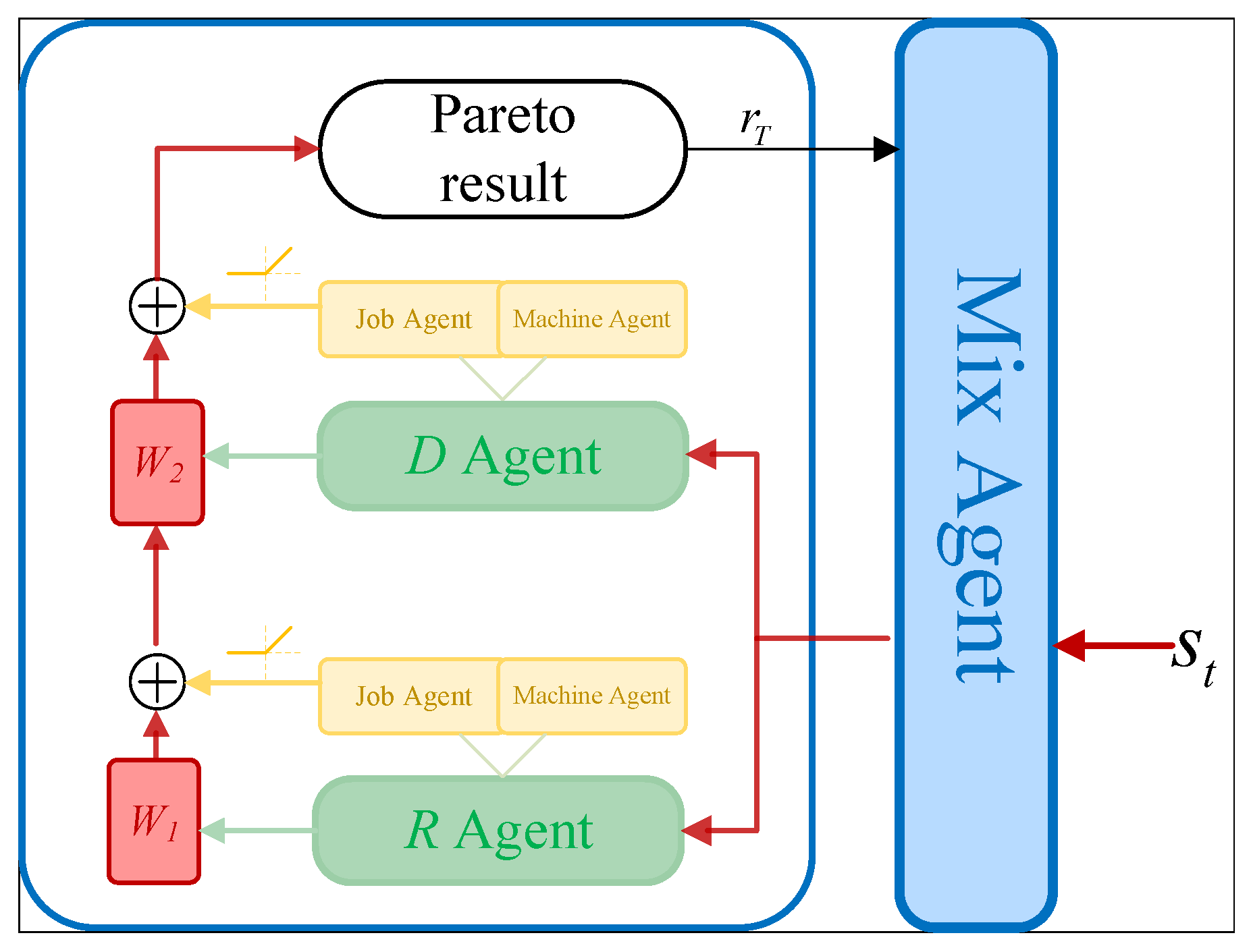
The dual-objective optimization algorithm based on hierarchical IDDQN-II proposed in this paper decouples the two optimization objectives during training. However, the two objectives must be reconnected during the testing processes to obtain the Pareto results. The adaptive weight method is a strategy for dynamically adjusting the weight coefficients of each objective function in multi-objective optimization problems. It aims to autonomously balance the competing relationships among different objectives based on the real-time solution set distribution or environmental conditions, thereby avoiding the bias in the optimization direction caused by fixed weights during training. The adaptive weight method is applied to the top-level agent in the hierarchical IDDQN-II framework to generate Pareto results. Moreover, makes it vary uniformly between the outputs of the two optimization objective agents, enabling the agent to explore the Pareto frontier more effectively. The output structure is shown in Figure 3.

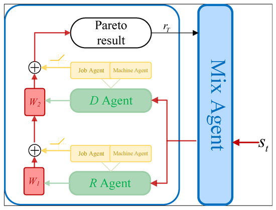
Figure 3. The output of Pareto results.

Each agent corresponds to a weight parameter, $W_1$ and $W_2$, where $W_1+W_2=1$. The action selection strategy in this paper is given by Equation (13).

$$a_t=\left\{\begin{array}{c}D\mathrm{Agent}\left(s_t\right),\mathrm{with}{W}_1\hfill \\ R\mathrm{Agent}\left(s_t\right),\mathrm{with}{W}_2\hfill \end{array}\right.$$

(13)

4. Computational Experiments and Results

This section conducts numerical simulations to validate the proposed algorithm’s effectiveness. IDDQN-II is coded in Python 3.9 with CUDA 11.3 and PyTorch (1.13.0). The running environment is on 12th Gen Intel® Core™i5-12500H @ 2.50 GHz, 40.00 GB RAM, RTX3060, Win11 64.

4.1. Experiment Preparation

The proposed IDDQN-II is trained in a simulated flexible job shop environment, the simulation data are generated based on the number of jobs $n\in \{5,10,15,20,30,50,100\}$, the number of machines $m\in \{5,10,15,20,30\}$. The proposed algorithm is evaluated on the standard benchmark. Some hyperparameters during training are shown in Table 2. These parameters are obtained by hyperparameter optimization using grid search. For example, some several sensitive hyperparameters, the learning rate is set to {0.1, 0.01, 0.001, 0.0001}, the number of iterations is {500, 1000, 1500, 2000, 2500, 3000}, and the discount factor is {0.95, 0.9, 0.85, 0.8, 0.75, 0.7}. After permuting and combining, the parameters that performed best are identified. Moreover, finer divisions within the interval should be made to confirm that no better parameters exist. The setting of coefficients in the greedy strategy $\theta$ enables the agent to effectively balance exploration and exploitation within a restricted number of iterations.

Table 2. The parameters of IDDQN-II.

Parameter	Value
Learning rate	0.01
Number of training iterations	$2\ast {10}^3$
The capacity of experience pool	$10\ast O_{sum}$
Sample batch size	$O_{sum}$
Coefficients in greedy strategy $\theta$	0.99 to 0.001
Update steps	$O_{sum}$
Discount factor $\gamma$	0.9
Prioritize experience replay alpha	0.6
Prioritize experience replay beta0	0.4
$W_1$	0.01 to 1

Table 3 outlines the instances utilized in the experiments. All benchmarks are static, assuming that all jobs are ready at the time of initialization. To ensure that tardiness is reflected in the evaluation of algorithmic performance and to prevent excessive flexibility in delivery times, the tardiness for each job is set at 80% of its average processing time, i.e., $D_i={\sum }_{j=0}^{n_i}{\displaystyle \frac{{\sum }_{k=1}^m{P}_{i,j,k}{X}_{i,j,k}}{|M_{i,j}|}}\ast 80\%$. It is noteworthy that tardiness is typically not as urgent as defined in this paper in the natural world’s production environment.

Table 3. Benchmark of testing and training.

Benchmark	Source
abz5, abz6, abz7, abz8, abz9	Adams et al. [30]
la30, la31, la32, la33, la34, la35	S [31]
mt06, mt10, mt20	H [32]
Mk01, Mk05, Mk10	Brandimarte [33]

4.2. Pareto Front Comparison Results and Analysis

This section compares the proposed DRL algorithm IDDQN-II with three commonly used multi-objective algorithms on the same test set to validate its effectiveness. Three widely used indicators Hypervolume (HV) [34], Spread (S) [35], and Inverted Generational Distance (IGD) [36] are adopted to comprehensively assess performance from multiple perspectives. HV can comprehensively assess an algorithm’s overall performance regarding convergence and distribution. IGD effectively measures convergence accuracy by calculating the distance between the solution set and the true Pareto frontier. Meanwhile, Spread specifically evaluates the uniformity of the solution set’s distribution. These three indicators represent essential dimensions in multi-objective optimization evaluation, and they are complementary and widely recognized in the field. Pareto results, often derived from Pareto efficiency or optimality, refer to outcomes in economic, decision-making, or multi-objective optimization scenarios where it is impossible to improve one criterion or individual’s situation without worsening another. These results are fundamental in evaluating resource allocation and strategic decisions across disciplines such as economics, game theory, and engineering. A solution is Pareto optimal if no other feasible solution can make at least one party better off without making someone else worse off. In practical applications—such as trade-offs between cost and performance in engineering design or policy evaluations—Pareto results are used to identify sets of non-dominated solutions, helping decision-makers visualize efficient frontiers and make informed, balanced choices among competing objectives.

A comparative experimental study is conducted using the multi-objective genetic algorithm (MOGA) [37], multi-objective particle swarm optimization (MOPSO) [38], and multi-objective differential evolution (MODE) [39]. The parameter settings for the three types of multi-objective optimization algorithms are determined using an orthogonal experimental approach. A medium-sized case study is selected, and each algorithm is executed 10 times. The optimal parameters are identified based on the best average performance observed. The parameter settings for MOGA $(populationsize,P_c,P_m)$ are (100, 0.85, 0.3), for MOPSO $(populationsize,w,c_1,c_2)$ are (150, 0.7, 0.5, 0.2), and for MODE $(populationsize,F,C_r)$ are (250, 0.5, 0.25). Since different algorithms require varying amounts of time for the same number of iterations, and DRL typically solves problems within seconds after training; this study uses CPU runtime(s) as the testing execution limit. The runtime for each algorithm is restricted to the product of the number of jobs and machines in the dataset. The final test results are summarized in Table 4, which highlights the best-performing outcomes in bold. The symbols “+”,“− ” and “=” indicate the significance of the analysis: “+” shows that IDDQN-II performs better, “−” indicates that the corresponding algorithm outperforms IDDQN-II on this test set, and “=” signifies that the performance of both algorithms is comparable.

Table 4. The comparison results of HV indicator.

Data	MOPSO		MOGA		MODE		IDDQN-II
abz5	$3.62\ast {10}^{-01}$	+	$7.31\ast {10}^{-01}$	+	$7.15\ast {10}^{-01}$	+	$\mathbf{8.71}\mathbf{\ast }{\mathbf{10}}^{\mathbf{-}\mathbf{01}}$
abz6	$3.30\ast {10}^{-01}$	+	$3.31\ast {10}^{-01}$	+	$3.02\ast {10}^{-01}$	+	$\mathbf{5.78}\mathbf{\ast }{\mathbf{10}}^{\mathbf{-}\mathbf{01}}$
abz7	$1.99\ast {10}^{-01}$	+	$7.33\ast {10}^{-01}$	−	$\mathbf{7.46}\mathbf{\ast }{\mathbf{10}}^{\mathbf{-}\mathbf{01}}$	−	$4.41\ast {10}^{-01}$
abz8	$1.26\ast {10}^{-01}$	+	$7.84\ast {10}^{-01}$	−	$\mathbf{8.04}\mathbf{\ast }{\mathbf{10}}^{\mathbf{-}\mathbf{01}}$	−	$6.58\ast {10}^{-01}$
abz9	$3.69\ast {10}^{-01}$	+	$2.40\ast {10}^{-01}$	+	$3.68\ast {10}^{-01}$	+	$\mathbf{5.92}\mathbf{\ast }{\mathbf{10}}^{\mathbf{-}\mathbf{01}}$
la30	$1.81\ast {10}^{-01}$	+	$4.98\ast {10}^{-01}$	−	$\mathbf{6.29}\mathbf{\ast }{\mathbf{10}}^{\mathbf{-}\mathbf{01}}$	−	$2.70\ast {10}^{-01}$
la31	$2.69\ast {10}^{-01}$	+	$1.49\ast {10}^{-01}$	+	$2.75\ast {10}^{-01}$	+	$\mathbf{3.21}\mathbf{\ast }{\mathbf{10}}^{\mathbf{-}\mathbf{01}}$
la32	$5.40\ast {10}^{-01}$	+	$3.78\ast {10}^{-01}$	+	$8.08\ast {10}^{-01}$	+	$\mathbf{9.09}\mathbf{\ast }{\mathbf{10}}^{\mathbf{-}\mathbf{01}}$
la33	$3.00\ast {10}^{-01}$	+	$3.07\ast {10}^{-01}$	+	$4.01\ast {10}^{-01}$	+	$\mathbf{4.64}\mathbf{\ast }{\mathbf{10}}^{\mathbf{-}\mathbf{01}}$
la34	$2.71\ast {10}^{-01}$	+	$2.93\ast {10}^{-01}$	+	$5.83\ast {10}^{-01}$	+	$\mathbf{9.37}\mathbf{\ast }{\mathbf{10}}^{\mathbf{-}\mathbf{01}}$
la35	$4.88\ast {10}^{-01}$	+	$2.22\ast {10}^{-01}$	+	$3.14\ast {10}^{-01}$	+	$\mathbf{5.09}\mathbf{\ast }{\mathbf{10}}^{\mathbf{-}\mathbf{01}}$
mt06	$\mathbf{8.98}\mathbf{\ast }{\mathbf{10}}^{\mathbf{-}\mathbf{01}}$	−	$6.83\ast {10}^{-01}$	−	$6.99\ast {10}^{-01}$	−	$4.42\ast {10}^{-01}$
mt10	$4.19\ast {10}^{-01}$	+	$4.47\ast {10}^{-01}$	+	$\mathbf{8.70}\mathbf{\ast }{\mathbf{10}}^{\mathbf{-}\mathbf{01}}$	−	$5.12\ast {10}^{-01}$
mt20	$4.29\ast {10}^{-01}$	+	$2.92\ast {10}^{-01}$	+	$\mathbf{6.96}\mathbf{\ast }{\mathbf{10}}^{\mathbf{-}\mathbf{01}}$	−	$5.32\ast {10}^{-01}$
Mk01	$5.95\ast {10}^{-01}$	−	$\mathbf{7.51}\mathbf{\ast }{\mathbf{10}}^{\mathbf{-}\mathbf{01}}$	−	$2.00\ast {10}^{-01}$	−	$1.61\ast {10}^{-01}$
Mk05	$5.96\ast {10}^{-01}$	+	$6.07\ast {10}^{-01}$	+	$7.79\ast {10}^{-01}$	+	$\mathbf{9.27}\mathbf{\ast }{\mathbf{10}}^{\mathbf{-}\mathbf{01}}$
Mk10	$4.72\ast {10}^{-01}$	+	$2.47\ast {10}^{-01}$	+	$2.94\ast {10}^{-01}$	+	$\mathbf{7.35}\mathbf{\ast }{\mathbf{10}}^{\mathbf{-}\mathbf{01}}$
+/−/=	15/2/0		12/5/0		10/7/0

Regarding the HV indicator, the proposed algorithm outperforms the baseline methods on at least 60% of the datasets. It demonstrates its advantage in global convergence and solution set diversity for multi-objective optimization. The improvement in HV can be attributed to two key mechanisms. First, the synergy between the attention mechanism and hierarchical action decoupling enables the algorithm to effectively explore the extended regions of the solution space, even under complex process constraints, thereby enhancing solution set coverage. The adaptive weight adjustment strategy helps address the common issue of local Pareto results aggregation in some DRL algorithms using fixed weights. This approach ensures a balanced trade-off between solution diversity, which involves maintaining a range of options across multiple objectives, and convergence, meaning how closely these solutions approach the true Pareto front.

The IGD indicator demonstrates that the proposed algorithm outperforms the compared algorithm on most benchmark datasets. It indicates that its dual-objective optimization results are closer to the true Pareto front, with improved convergence and more uniform distribution. The better results in IGD are primarily attributed to decoupling the two optimization objectives during training, allowing them to be learned independently. This is unlike some DRL-based approaches that assign fixed weights to optimization objectives, which will constrain the agent’s exploration of the solution space due to conflicting objectives and achieve a worse close with the true Pareto front (Table 5 and Table 6).

Table 5. The comparison results of IGD indicator.

Data	MOPSO		MOGA		MODE		IDDQN-II
abz5	$7.69\ast {10}^{-01}$	+	$3.38\ast {10}^{-01}$	−	$\mathbf{2.13}\mathbf{\ast }{\mathbf{10}}^{\mathbf{-}\mathbf{01}}$	−	$5.53\ast {10}^{-01}$
abz6	$7.61\ast {10}^{-01}$	+	$5.27\ast {10}^{-01}$	+	$5.68\ast {10}^{-01}$	+	$\mathbf{1.20}\mathbf{\ast }{\mathbf{10}}^{\mathbf{-}\mathbf{01}}$
abz7	$8.50\ast {10}^{-01}$	+	$\mathbf{1.20}\mathbf{\ast }{\mathbf{10}}^{\mathbf{-}\mathbf{01}}$	−	$7.92\ast {10}^{-01}$	+	$4.38\ast {10}^{-01}$
abz8	$8.89\ast {10}^{-01}$	+	$2.28\ast {10}^{-01}$	+	$4.08\ast {10}^{-01}$	+	$\mathbf{1.70}\mathbf{\ast }{\mathbf{10}}^{\mathbf{-}\mathbf{01}}$
abz9	$8.72\ast {10}^{-01}$	+	$7.82\ast {10}^{-01}$	+	$4.22\ast {10}^{-01}$	+	$\mathbf{1.00}\mathbf{\ast }{\mathbf{10}}^{\mathbf{-}\mathbf{02}}$
la30	$1.10\ast {10}^{+00}$	+	$4.48\ast {10}^{-01}$	+	$4.69\ast {10}^{-01}$	+	$\mathbf{1.30}\mathbf{\ast }{\mathbf{10}}^{\mathbf{-}\mathbf{01}}$
la31	$8.92\ast {10}^{-01}$	+	$4.43\ast {10}^{-01}$	+	$4.50\ast {10}^{-01}$	+	$\mathbf{3.44}\mathbf{\ast }{\mathbf{10}}^{\mathbf{-}\mathbf{01}}$
la32	$8.24\ast {10}^{-01}$	+	$5.20\ast {10}^{-01}$	+	$2.86\ast {10}^{-01}$	+	$\mathbf{2.09}\mathbf{\ast }{\mathbf{10}}^{\mathbf{-}\mathbf{01}}$
la33	$8.12\ast {10}^{-01}$	+	$4.33\ast {10}^{-01}$	+	$3.72\ast {10}^{-01}$	+	$\mathbf{1.12}\mathbf{\ast }{\mathbf{10}}^{\mathbf{-}\mathbf{01}}$
la34	$7.72\ast {10}^{-01}$	+	$5.00\ast {10}^{-01}$	+	$3.35\ast {10}^{-01}$	+	$\mathbf{2.08}\mathbf{\ast }{\mathbf{10}}^{\mathbf{-}\mathbf{01}}$
la35	$5.50\ast {10}^{-01}$	+	$5.20\ast {10}^{-01}$	+	$4.77\ast {10}^{-01}$	+	$\mathbf{7.50}\mathbf{\ast }{\mathbf{10}}^{\mathbf{-}\mathbf{02}}$
mt06	$\mathbf{1.95}\mathbf{\ast }{\mathbf{10}}^{\mathbf{-}\mathbf{01}}$	−	$3.01\ast {10}^{-01}$	−	$2.98\ast {10}^{-01}$	−	$3.36\ast {10}^{-01}$
mt10	$3.86\ast {10}^{-01}$	+	$4.00\ast {10}^{-01}$	+	$\mathbf{2.07}\mathbf{\ast }{\mathbf{10}}^{\mathbf{-}\mathbf{01}}$	−	$2.64\ast {10}^{-01}$
mt20	$9.69\ast {10}^{-01}$	+	$3.64\ast {10}^{-01}$	+	$2.49\ast {10}^{-01}$	+	$\mathbf{1.69}\mathbf{\ast }{\mathbf{10}}^{\mathbf{-}\mathbf{01}}$
Mk01	$3.11\ast {10}^{-01}$	−	$\mathbf{1.01}\mathbf{\ast }{\mathbf{10}}^{\mathbf{-}\mathbf{01}}$	−	$7.48\ast {10}^{-01}$	−	$8.78\ast {10}^{-01}$
Mk05	$8.39\ast {10}^{-01}$	+	$\mathbf{2.42}\mathbf{\ast }{\mathbf{10}}^{\mathbf{-}\mathbf{01}}$	−	$4.43\ast {10}^{-01}$	+	$3.67\ast {10}^{-01}$
Mk10	$6.48\ast {10}^{-01}$	+	$6.22\ast {10}^{-01}$	+	$6.11\ast {10}^{-01}$	+	$\mathbf{2.18}\mathbf{\ast }{\mathbf{10}}^{\mathbf{-}\mathbf{01}}$
+/−/=	15/2/0		12/5/0		13/4/0

Table 6. The comparison results of Spread indicator.

Data	MOPSO		MOGA		MODE		IDDQN-II
abz5	$8.83\ast {10}^{-02}$	+	$\mathbf{4.31}\mathbf{\ast }{\mathbf{10}}^{\mathbf{-}\mathbf{01}}$	−	$1.45\ast {10}^{-01}$	+	$3.77\ast {10}^{-01}$
abz6	$6.03\ast {10}^{-02}$	+	$3.80\ast {10}^{-01}$	+	$2.53\ast {10}^{-01}$	+	$\mathbf{4.46}\mathbf{\ast }{\mathbf{10}}^{\mathbf{-}\mathbf{01}}$
abz7	$3.23\ast {10}^{-01}$	+	$3.73\ast {10}^{-01}$	+	$1.48\ast {10}^{-01}$	+	$\mathbf{4.77}\mathbf{\ast }{\mathbf{10}}^{\mathbf{-}\mathbf{01}}$
abz8	$3.04\ast {10}^{-01}$	+	$2.36\ast {10}^{-01}$	+	$2.04\ast {10}^{-01}$	+	$\mathbf{3.80}\mathbf{\ast }{\mathbf{10}}^{\mathbf{-}\mathbf{01}}$
abz9	$1.33\ast {10}^{-01}$	+	$1.20\ast {10}^{-01}$	+	$2.57\ast {10}^{-01}$	+	$\mathbf{4.74}\mathbf{\ast }{\mathbf{10}}^{\mathbf{-}\mathbf{01}}$
la30	$8.69\ast {10}^{-02}$	+	$2.45\ast {10}^{-01}$	+	$1.61\ast {10}^{-01}$	+	$\mathbf{6.23}\mathbf{\ast }{\mathbf{10}}^{\mathbf{-}\mathbf{01}}$
la31	$8.62\ast {10}^{-02}$	+	$3.21\ast {10}^{-01}$	+	$2.75\ast {10}^{-01}$	+	$\mathbf{5.84}\mathbf{\ast }{\mathbf{10}}^{\mathbf{-}\mathbf{01}}$
la32	$1.24\ast {10}^{-01}$	+	$1.54\ast {10}^{-01}$	+	$\mathbf{3.22}\mathbf{\ast }{\mathbf{10}}^{\mathbf{-}\mathbf{01}}$	−	$2.67\ast {10}^{-01}$
la33	$9.32\ast {10}^{-02}$	+	$1.86\ast {10}^{-01}$	+	$1.72\ast {10}^{-01}$	+	$\mathbf{5.09}\mathbf{\ast }{\mathbf{10}}^{\mathbf{-}\mathbf{01}}$
la34	$2.17\ast {10}^{-01}$	+	$1.10\ast {10}^{-01}$	+	$1.54\ast {10}^{-01}$	+	$\mathbf{2.28}\mathbf{\ast }{\mathbf{10}}^{\mathbf{-}\mathbf{01}}$
la35	$1.67\ast {10}^{-01}$	+	$2.46\ast {10}^{-01}$	+	$1.85\ast {10}^{-01}$	+	$\mathbf{4.73}\mathbf{\ast }{\mathbf{10}}^{\mathbf{-}\mathbf{01}}$
mt06	$2.57\ast {10}^{-01}$	+	$\mathbf{3.23}\mathbf{\ast }{\mathbf{10}}^{\mathbf{-}\mathbf{01}}$	−	$1.88\ast {10}^{-01}$	+	$3.06\ast {10}^{-01}$
mt10	$2.65\ast {10}^{-01}$	+	$1.45\ast {10}^{-01}$	+	$1.39\ast {10}^{-01}$	+	$\mathbf{3.36}\mathbf{\ast }{\mathbf{10}}^{\mathbf{-}\mathbf{01}}$
mt20	$9.91\ast {10}^{-02}$	+	$1.79\ast {10}^{-01}$	+	$1.64\ast {10}^{-01}$	+	$\mathbf{4.60}\mathbf{\ast }{\mathbf{10}}^{\mathbf{-}\mathbf{01}}$
Mk01	$2.21\ast {10}^{-01}$	−	$1.82\ast {10}^{-01}$	−	$\mathbf{2.24}\mathbf{\ast }{\mathbf{10}}^{\mathbf{-}\mathbf{01}}$	−	$1.70\ast {10}^{-01}$
Mk05	$1.38\ast {10}^{-01}$	+	$1.69\ast {10}^{-01}$	+	$2.38\ast {10}^{-01}$	+	$\mathbf{3.85}\mathbf{\ast }{\mathbf{10}}^{\mathbf{-}\mathbf{01}}$
Mk10	$1.08\ast {10}^{-01}$	+	$2.52\ast {10}^{-01}$	−	$\mathbf{3.04}\mathbf{\ast }{\mathbf{10}}^{\mathbf{-}\mathbf{01}}$	−	$2.35\ast {10}^{-01}$
+/−/=	16/1/0		13/4/0		14/3/0

The proposed IDDQN-II outperforms others in terms of the S indicator, indicating superior solution uniformity and the ability to adapt more effectively to diverse scheduling scenarios.

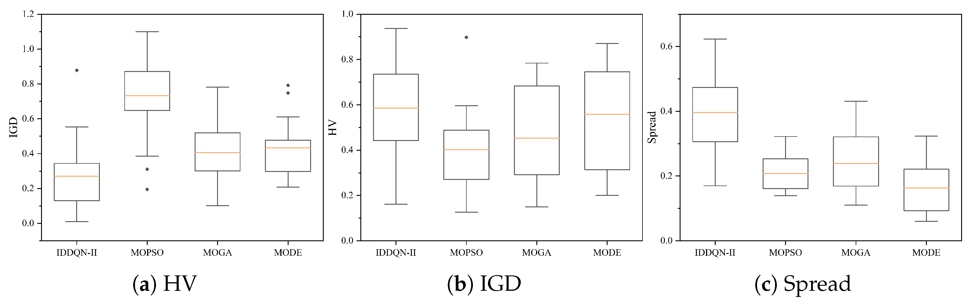
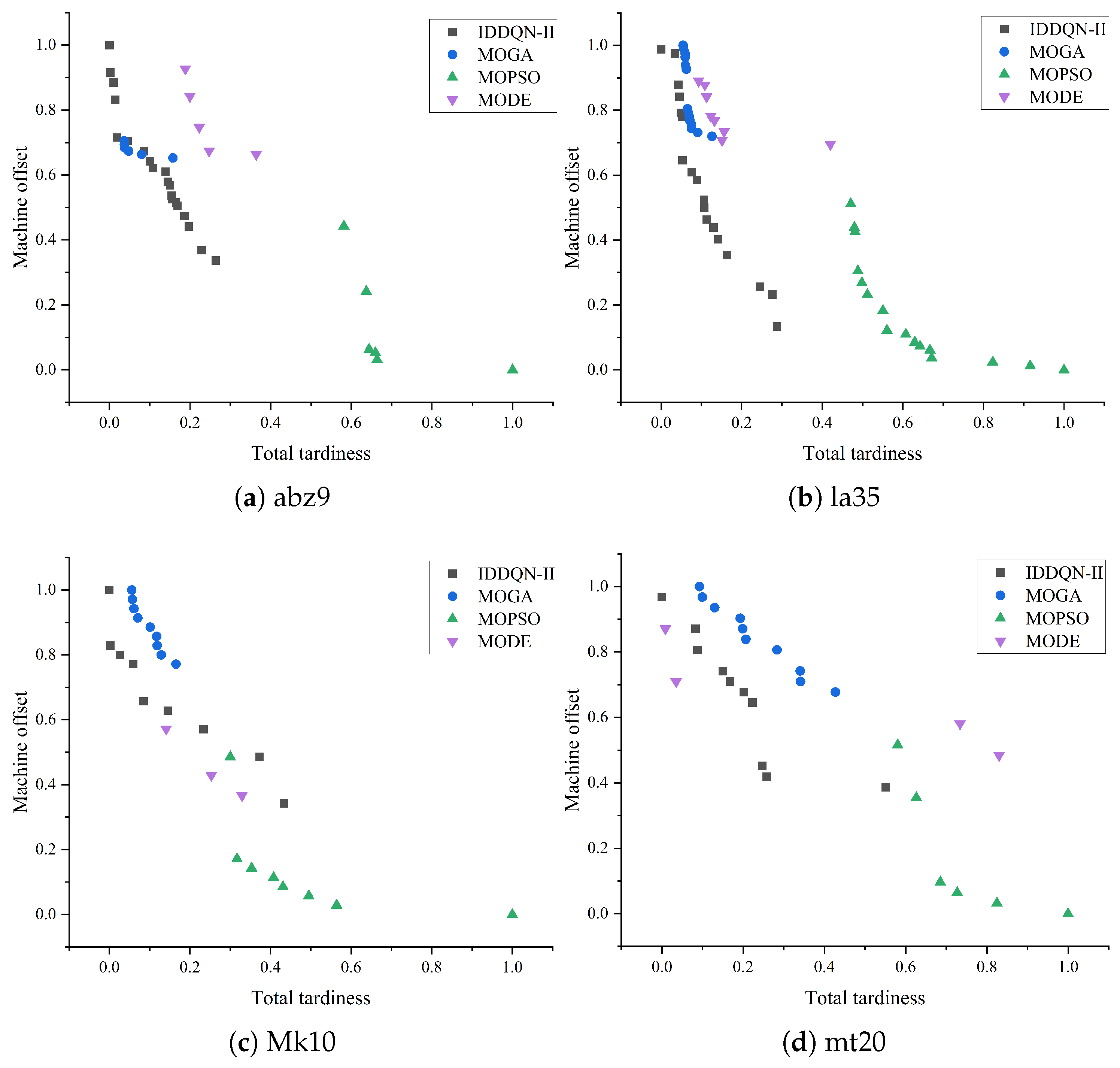
The box plot in Figure 4 shows that IDDQN-II excels across all three indicators, which is unusual in previous research because agents, the core of deep reinforcement learning, frequently find it difficult to learn complex multi-objective relationships. The scatter plot Figure 5 shows that IDDQN-II exhibits greater stability in different datasets from the benchmark and explores a broader set of Pareto results. The scatter plot indicates that IDDQN-II obtains more Pareto results within limited run times, which are better distributed and nearer to the lower-left corner.

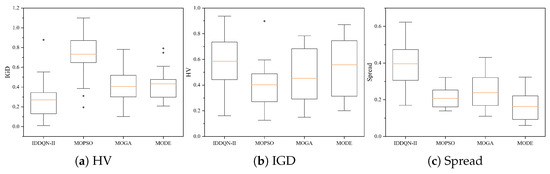
Figure 4. Box plot of benchmark.

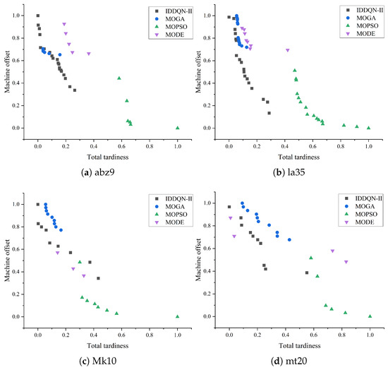
Figure 5. Scatter plot of representative datasets from the benchmark.

The results indicate that in addressing the dual-objective rescheduling problem of flexible job shops under dynamic machine breakdown, the adaptive weight adjustment method effectively balances the agent’s action output for different optimization objectives, leading to high-quality Pareto results. Decoupling job and machine selection in the algorithm expands the solution space while reducing problem complexity. Additionally, embedding an attention mechanism enhances the agent’s ability to process large-scale state features efficiently.

4.3. Validation Using Real Case from Enterprises

To further validate the effectiveness of the proposed algorithm, this paper conducted a case study using real-world data from a manufacturing enterprise. The case study involved a FJSP with dynamic machine breakdowns. The enterprise produces a variety of products with different processing requirements, and the scheduling process is subject to frequent machine breakdowns.

4.3.1. Case Study Description

The manufacturing industry for building materials and equipment plays a vital role in the Chinese economy [40]. The building materials industry represents 7% of total energy consumption, while its economic impact accounts for 9% of the overall economic weight [41]. It focuses on producing heavy machinery, including tube mills, rotary kilns, and vertical mills. These machines are widely used in cement, metallurgy, and related sectors for processes such as raw material crushing, grinding, and thermal processing. This study selects the manufacturing industry for building materials and equipment as a case for flexible job shop scheduling due to its strong alignment with the research focus. The industry is characterized by large-scale, modular, and highly customized production equipment, with component manufacturing involving a complex process chain, including fundamental shaping (“scribing–turning–boring”), precision machining (“milling–drilling–rolling”), and heat treatment. A single product may require over 20 sequential operations, forming a nested multiprocess system. Additionally, production in this industry inherently exhibits equipment heterogeneity, with process routes integrating diverse manufacturing methods such as casting, welding, and machining, necessitating intricate coordination between CNC machine tools and specialized welding equipment.

The current process of the manufacturing industry for building materials and equipment includes several key aspects: the military enterprise, the push for accelerated promotion, the digitalization of manufacturing systems, and the strategic approach to structural strategy. This approach enables the development of an advanced manufacturing model that integrates standardized bidding, centralized procurement, and intelligent scheduling. The innovative production process architecture is illustrated in Figure 6. The marketing department of the enterprise obtains production orders through market bidding and creates a project plan for task decomposition. Initially, the technical department carries out the necessary preparations based on the order requirements. This includes creating product design drawings, specifications, and parameters, as well as producing detailed lists of materials and generating accurate purchase lists. Then, the storage and transportation department manages the existing material inventory according to the purchase list and communicates the purchasing requirements to the purchasing department. The purchasing department then executes the process of inquiring about market prices and compares options based on the purchasing requirements and the material lists, while also considering potential material substitutions. Following this, the production department translates the detailed production requirements into a scheduling plan to guide the workshop’s production. They establish a reasonable production plan using efficient optimization algorithms, which is then sent to the workshop. Additionally, the production department can generate a rescheduling plan in real time in response to dynamic events in the job shop, minimizing losses caused by unexpected changes.

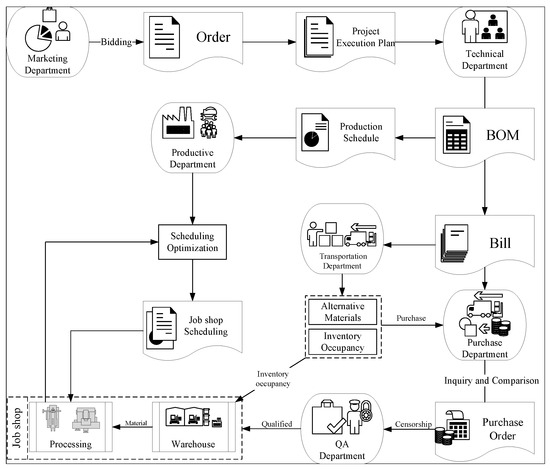
Figure 6. The process of the manufacturing industry for building materials and equipment.

This research thoroughly surveys a leading domestic construction materials equipment manufacturer as a case study, selecting 13 representative product categories and 65 key jobs to construct the dynamic scheduling environment. Appendix A provides detailed information on machining equipment and job process. A comparative analysis is conducted between the proposed IDDQN-II and classical multi-objectives optimization algorithm to evaluate their effectiveness and solution performance in flexible job shop rescheduling for natural production. The findings offer a practical technical solution to address the multi-objective scheduling challenges specific to the construction materials equipment industry, particularly for non-standard parts.

4.3.2. Experimental Validation Results

Due to the large volume of materials in the production process and the difficulty of transportation, rescheduling leads to an offset between the processing machines and the initial scheduling plan, resulting in additional resource overhead. Meanwhile, some operations require preparing materials and transporting them to processing machines, where they await processing. This section compares the IDDQN-II and three commonly used optimization algorithms in the scheduling environment constructed to minimize total job tardiness and minimize machine offset. The algorithm parameters are set as in Section 4.2. Each of the four algorithms is run 20 times, and the results obtained from these are presented in Table 7.

Table 7. The results of the natural case.

Indicators	Algorithms
	IDDQN-II	MOGA	MOPSO	MODE
HV	$\mathbf{9.00}\mathbf{\ast }{\mathbf{10}}^{\mathbf{-}\mathbf{01}}$	$2.90\ast {10}^{-01}$	$7.86\ast {10}^{-01}$	$3.02\ast {10}^{-01}$
IGD	$2.08\ast {10}^{-01}$	$5.51\ast {10}^{-01}$	$\mathbf{1.79}\mathbf{\ast }{\mathbf{10}}^{\mathbf{-}\mathbf{01}}$	$4.55\ast {10}^{-01}$
Spread	$\mathbf{1.53}\mathbf{\ast }{\mathbf{10}}^{\mathbf{-}\mathbf{01}}$	$1.11\ast {10}^{-01}$	$1.32\ast {10}^{-01}$	$1.25\ast {10}^{-01}$

Table 7 shows that the best HV obtained by IDDQN-II finds a higher quality of non-dominated solution set in the solution space, indicating that the algorithm’s optimization ability performs equally well in the natural case. Although slightly inferior to MOPSO in the IGD indicator, the difference between them is minimal, and the proposed algorithm excels in the Spread indicators.

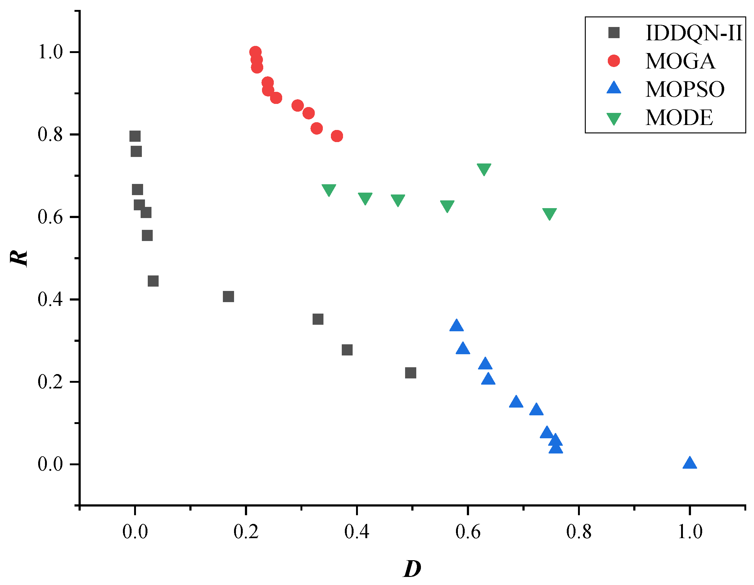
To provide a more straightforward illustration of the Pareto front solutions from each algorithm, Figure 7 presents a scatter plot of the Pareto solutions. The x-axis represents the normalized total job tardiness, while the y-axis represents the normalized machine offset. The figure shows that the Pareto results obtained by IDDQN-II are closer to the lower left corner, indicating that the algorithm achieves a higher solution quality when addressing dual-objective optimization. Additionally, the shape of the Pareto results produced by the algorithm resembles a smooth curve without significant fluctuations. This demonstrates that the proposed algorithm effectively balances the two optimization goals: minimizing the total delay of jobs and reducing machine offset. The algorithm provides only a set of feasible Pareto results. In a practical production environment, schedulers can select the most suitable scheduling plan based on multi-attribute decision-making methods or specific needs.

Figure 7. The Pareto scatter plot of natural case.

5. Conclusions and Future Work

This study addresses the complex and highly relevant issue of rescheduling in flexible job shop environments, particularly under dynamic conditions with machine breakdowns. To tackle the dual-objective optimization challenge—minimizing makespan and improving machine offset—this paper proposed an improved deep reinforcement learning algorithm, IDDQN-II. The unique multi-level structure enables agents to learn different optimization objectives and enhances learning efficiency by combining sparse rewards. Additionally, it facilitates more complex dispatch rule combinations while reducing the action space that each agent must explore.

The experimental results demonstrate that IDDQN-II significantly outperforms three commonly used metaheuristic algorithms regarding solution quality and adaptability to disruptions. This highlights the practical advantages of leveraging deep reinforcement learning techniques in highly dynamic and uncertain production settings. Our approach enhances production efficiency and provides a flexible framework that can adapt to changes in real time, making it suitable for industrial implementation. The model effectively captures practical constraints and scheduling requirements by testing real-world data from a manufacturing enterprise in the building materials and equipment industry.

However, several limitations should be acknowledged. First, while the model considers machine breakdowns a key dynamic factor, other unpredictable events such as urgent order insertions, workforce constraints, or supply chain disruptions were not included in the current framework. Additionally, the model’s performance has only been validated on data from a single industry sector, which may limit the generalizability of the results across different production environments.

Future research will enhance the model’s robustness and applicability by incorporating more diverse dynamic factors and additional optimization objectives, such as energy consumption, cost, and human factors. Furthermore, extending the algorithm to accommodate multi-factory collaboration or real-time rescheduling under Industry 5.0 scenarios could further improve its practical impact. Combining our approach with digital twin technologies or edge computing for real-time decision-making also represents a promising direction for industrial applications.

References

- Li, R.; Gong, W.; Wang, L.; Lu, C.; Dong, C. Co-Evolution with Deep Reinforcement Learning for Energy-Aware Distributed Heterogeneous Flexible Job Shop Scheduling. IEEE Trans. Syst. Man Cybern. Syst. 2024, 54, 201–211. [Google Scholar] [CrossRef]
- Dauzère-Pérès, S.; Ding, J.; Shen, L.; Tamssaouet, K. The Flexible Job Shop Scheduling Problem: A Review. Eur. J. Oper. Res. 2023, 314, S037722172300382X. [Google Scholar] [CrossRef]
- Jiang, B.; Ma, Y.; Chen, L.; Huang, B.; Huang, Y.; Guan, L. A Review on Intelligent Scheduling and Optimization for Flexible Job Shop. Int. J. Control. Autom. Syst. 2023, 21, 3127–3150. [Google Scholar] [CrossRef]
- Yao, Y.J.; Liu, Q.H.; Li, X.Y.; Gao, L. A Novel MILP Model for Job Shop Scheduling Problem with Mobile Robots. Robot. Comput.-Integr. Manuf. 2023, 81, 102506. [Google Scholar] [CrossRef]
- Shi, S.; Xiong, H. Solving the Multi-Objective Job Shop Scheduling Problems with Overtime Consideration by an Enhanced NSGA-II. Comput. Ind. Eng. 2024, 190, 110001. [Google Scholar] [CrossRef]
- Ding, J.; Chen, M.; Wang, T.; Zhou, J.; Fu, X.; Li, K. A Survey of AI-enabled Dynamic Manufacturing Scheduling: From Directed Heuristics to Autonomous Learning. ACM Comput. Surv. 2023, 55, 307:1–307:36. [Google Scholar] [CrossRef]
- Tariq, A.; Khan, S.A.; But, W.H.; Javaid, A.; Shehryar, T. An IoT-enabled Real-Time Dynamic Scheduler for Flexible Job Shop Scheduling (FJSS) in an Industry 4.0-Based Manufacturing Execution System (MES 4.0). IEEE Access 2024, 12, 49653–49666. [Google Scholar] [CrossRef]
- Liu, A.; Luh, P.B.; Sun, K.; Bragin, M.A.; Yan, B. Integrating Machine Learning and Mathematical Optimization for Job Shop Scheduling. IEEE Trans. Autom. Sci. Eng. 2024, 21, 4829–4850. [Google Scholar] [CrossRef]
- Huang, G.; Hu, M.; Yang, X.; Lin, P.; Wang, Y. Addressing Constraint Coupling and Autonomous Decision-Making Challenges: An Analysis of Large-Scale UAV Trajectory-Planning Techniques. Drones 2024, 8, 530. [Google Scholar] [CrossRef]
- Wang, J.; Liu, Y.; Ren, S.; Wang, C.; Ma, S. Edge Computing-Based Real-Time Scheduling for Digital Twin Flexible Job Shop with Variable Time Window. Robot. Comput.-Integr. Manuf. 2023, 79, 102435. [Google Scholar] [CrossRef]
- Destouet, C.; Tlahig, H.; Bettayeb, B.; Mazari, B. Flexible Job Shop Scheduling Problem under Industry 5.0: A Survey on Human Reintegration, Environmental Consideration and Resilience Improvement. J. Manuf. Syst. 2023, 67, 155–173. [Google Scholar] [CrossRef]
- Yao, Y.; Wang, Q.; Wang, C.; Li, X.; Gao, L.; Xia, K. Knowledge-Based Multi-Objective Evolutionary Algorithm for Energy-Efficient Flexible Job Shop Scheduling with Mobile Robot Transportation. Adv. Eng. Inform. 2024, 62, 102647. [Google Scholar] [CrossRef]
- Sun, J.; Zhang, Z.; Zhang, G.; Huang, Z. Multi-Objective Evolutionary Algorithm Based Flexible Assembly Job-Shop Rescheduling with Component Sharing for Order Insertion. Comput. Oper. Res. 2024, 169, 106744. [Google Scholar] [CrossRef]
- Xie, J.; Li, X.; Gao, L.; Gui, L. A Hybrid Genetic Tabu Search Algorithm for Distributed Flexible Job Shop Scheduling Problems. J. Manuf. Syst. 2023, 71, 82–94. [Google Scholar] [CrossRef]
- Burmeister, S.C.; Guericke, D.; Schryen, G. A Memetic NSGA-II for the Multi-Objective Flexible Job Shop Scheduling Problem with Real-Time Energy Tariffs. Flex. Serv. Manuf. J. 2024, 36, 1530–1570. [Google Scholar] [CrossRef]
- Zhang, F.; Shi, G.; Mei, Y.; Zhang, M. Multiobjective Dynamic Flexible Job Shop Scheduling with Biased Objectives via Multitask Genetic Programming. IEEE Trans. Artif. Intell. 2025, 6, 169–183. [Google Scholar] [CrossRef]
- Gui, Y.; Tang, D.; Zhu, H.; Zhang, Y.; Zhang, Z. Dynamic Scheduling for Flexible Job Shop Using a Deep Reinforcement Learning Approach. Comput. Ind. Eng. 2023, 180, 109255. [Google Scholar] [CrossRef]
- Hammami, N.E.H.; Lardeux, B.; Hadj-Alouane, A.B.; Jridi, M. Design and Calibration of a DRL Algorithm for Solving the Job Shop Scheduling Problem under Unexpected Job Arrivals. Flex. Serv. Manuf. J. 2024. [Google Scholar] [CrossRef]
- Zhao, L.; Fan, J.; Zhang, C.; Shen, W.; Zhuang, J. A DRL-based Reactive Scheduling Policy for Flexible Job Shops with Random Job Arrivals. IEEE Trans. Autom. Sci. Eng. 2024, 21, 2912–2923. [Google Scholar] [CrossRef]
- Gan, X.; Zuo, Y.; Yang, G.; Zhang, A.; Tao, F. Dynamic Scheduling for Dual-Objective Job Shop with Machine Breakdown by Reinforcement Learning. Proc. Inst. Mech. Eng. Part B J. Eng. Manuf. 2024, 238, 3–17. [Google Scholar] [CrossRef]
- Das, K. A Comparative Study of Exponential Distribution vs. Weibull Distribution in Machine Reliability Analysis in a CMS Design. Comput. Ind. Eng. 2008, 54, 12–33. [Google Scholar] [CrossRef]
- Chen, J.; Zhao, Y.; Wang, M.; Yang, K.; Ge, Y.; Wang, K.; Lin, H.; Pan, P.; Hu, H.; He, Z.; et al. Multi-Timescale Reward-Based DRL Energy Management for Regenerative Braking Energy Storage System. IEEE Trans. Transp. Electrif. 2025. early access. [Google Scholar] [CrossRef]
- Nguyen, T.T.; Nguyen, N.D.; Vamplew, P.; Nahavandi, S.; Dazeley, R.; Lim, C.P. A Multi-Objective Deep Reinforcement Learning Framework. Eng. Appl. Artif. Intell. 2020, 96, 103915. [Google Scholar] [CrossRef]
- Lu, S.; Wang, Y.; Kong, M.; Wang, W.; Tan, W.; Song, Y. A Double Deep Q-Network Framework for a Flexible Job Shop Scheduling Problem with Dynamic Job Arrivals and Urgent Job Insertions. Eng. Appl. Artif. Intell. 2024, 133, 108487. [Google Scholar] [CrossRef]
- Dorfman, R. A Formula for the Gini Coefficient. Rev. Econ. Stat. 1979, 61, 146–149. [Google Scholar] [CrossRef]
- Vaswani, A.; Shazeer, N.; Parmar, N.; Uszkoreit, J.; Jones, L.; Gomez, A.N.; Kaiser, L.; Polosukhin, I. Attention Is All You Need. arXiv 2023, arXiv:1706.03762. [Google Scholar] [CrossRef]
- Doh, H.H.; Yu, J.M.; Kim, J.S.; Lee, D.H.; Nam, S.H. A Priority Scheduling Approach for Flexible Job Shops with Multiple Process Plans. Int. J. Prod. Res. 2013, 51, 3748–3764. [Google Scholar] [CrossRef]
- Jeong, K.C.; Kim, Y.D. A Real-Time Scheduling Mechanism for a Flexible Manufacturing System: Using Simulation and Dispatching Rules. Int. J. Prod. Res. 1998, 36, 2609–2626. [Google Scholar] [CrossRef]
- Priore, P.; Ponte, B.; Puente, J.; Gómez, A. Learning-Based Scheduling of Flexible Manufacturing Systems Using Ensemble Methods. Comput. Ind. Eng. 2018, 126, 282–291. [Google Scholar] [CrossRef]
- Adams, J.; Balas, E.; Zawack, D. The Shifting Bottleneck Procedure for Job Shop Scheduling. Manag. Sci. 1988, 34, 391–401. [Google Scholar] [CrossRef]
- Lawrence, S. Resouce Constrained Project Scheduling: An Experimental Investigation of Heuristic Scheduling Techniques (Supplement); Graduate School of Industrial Administration, Carnegie-Mellon University: Pittsburgh, PA, USA, 1984. [Google Scholar]
- Fisher, H.; Thompson, G.L. Probabilistic Learning Combinations of Local Job-Shop Scheduling Rules. In Industrial Scheduling; Muth, J.F., Thompson, G.L., Eds.; Prentice-Hall: Englewood Cliffs, NJ, USA, 1963; pp. 225–251. [Google Scholar]
- Brandimarte, P. Routing and Scheduling in a Flexible Job Shop by Tabu Search. Ann. Oper. Res. 1993, 41, 157–183. [Google Scholar] [CrossRef]
- Shang, K.; Ishibuchi, H.; He, L.; Pang, L.M. A Survey on the Hypervolume Indicator in Evolutionary Multiobjective Optimization. IEEE Trans. Evol. Comput. 2021, 25, 1–20. [Google Scholar] [CrossRef]
- He, L.; Chiong, R.; Li, W.; Dhakal, S.; Cao, Y.; Zhang, Y. Multiobjective Optimization of Energy-Efficient JOB-shop Scheduling with Dynamic Reference Point-Based Fuzzy Relative Entropy. IEEE Trans. Ind. Inform. 2022, 18, 600–610. [Google Scholar] [CrossRef]
- Sun, Y.; Yen, G.G.; Yi, Z. IGD Indicator-Based Evolutionary Algorithm for Many-Objective Optimization Problems. IEEE Trans. Evol. Comput. 2019, 23, 173–187. [Google Scholar] [CrossRef]
- Yin, L.; Li, X.; Gao, L.; Lu, C.; Zhang, Z. A Novel Mathematical Model and Multi-Objective Method for the Low-Carbon Flexible Job Shop Scheduling Problem. Sustain. Comput. Inform. Syst. 2017, 13, 15–30. [Google Scholar] [CrossRef]
- Esmaeilion, F.; Ahmadi, A.; Dashti, R. Exergy-Economic-Environment Optimization of the Waste-to-Energy Power Plant Using Multi-Objective Particle-Swarm Optimization (MOPSO). Sci. Iran. 2021, 28, 2733–2750. [Google Scholar] [CrossRef]
- Xiao, B.; Zhao, Z.; Wu, Y.; Zhu, X.; Peng, S.; Su, H. An Improved MOEA/D for Multi-Objective Flexible Job Shop Scheduling by Considering Efficiency and Cost. Comput. Oper. Res. 2024, 167, 106674. [Google Scholar] [CrossRef]
- Sun, Y.; Wang, J.; Wang, X. Fault Diagnosis of Mechanical Equipment in High Energy Consumption Industries in China: A Review. Mech. Syst. Signal Process. 2023, 186, 109833. [Google Scholar] [CrossRef]
- Ramakrishna Balaji, C.; de Azevedo, A.R.G.; Madurwar, M. Sustainable Perspective of Ancillary Construction Materials in Infrastructure Industry: An Overview. J. Clean. Prod. 2022, 365, 132864. [Google Scholar] [CrossRef]
Disclaimer/Publisher’s Note: The statements, opinions and data contained in all publications are solely those of the individual author(s) and contributor(s) and not of MDPI and/or the editor(s). MDPI and/or the editor(s) disclaim responsibility for any injury to people or property resulting from any ideas, methods, instructions or products referred to in the content. |
© 2025 by the authors. Licensee MDPI, Basel, Switzerland. This article is an open access article distributed under the terms and conditions of the Creative Commons Attribution (CC BY) license (https://creativecommons.org/licenses/by/4.0/).