Abstract
Active frequency response (AFR) plays a crucial role in addressing the challenge of insufficient frequency regulation caused by the spatiotemporal distribution of power grid frequency. However, power fluctuations in renewable energy sources impact the frequency regulation performance of renewable energy units participating in AFR, and there is a lack of systematic assessment of their frequency regulation capabilities. This paper proposes a process-optimized AFR method for renewable energy based on distributed model predictive control (DMPC) using tube and robust control barrier functions (RCBF). The method integrates tube MPC for renewable energy units in fault regions and constrains control parameters in normal regions using RCBF, forming an enhanced DMPC-based coordination process for interconnected systems. This optimization ensures that both conventional and renewable energy units can effectively perform AFR under fluctuating renewable energy conditions. Furthermore, within the AFR online decision-making process, the optimal deloading rate for renewable energy is determined to maintain sufficient power reserves and frequency regulation capabilities. Finally, simulations of an interconnected system with a high proportion of renewable energy validate the effectiveness of this process-driven approach in enhancing the AFR capabilities of renewable energy sources.
1. Introduction
With the expansion of the power grid scale and the complication of its structure, the frequency in the interconnected power grid shows obvious spatio-temporal differences [1]. A large number of renewable energy sources are connected to the power grid. As this occurs, the uneven distribution of inertia increases. This increase in uneven inertia distribution leads to another consequence. Specifically, after a fault, the spatio-temporal distribution of the system frequency becomes more prominent: the farther away from the fault node, the slower the frequency change [2]. This poses new requirements for renewable energy sources to participate in frequency regulation [3].
The existing frequency regulation of renewable energy generally relies on the decentralized time-difference frequency control method based on local measurements and preset parameters [4,5,6,7]. The traditional approach is decentralized control. However, it has two main issues: primary frequency regulation lags due to frequency’s spatio-temporal differences, and frequency regulation resources are not fully utilized. Moreover, its response speed and control accuracy cannot meet the requirements.
AFR can leverage real-time data from the wide-area measurement system. It can then mobilize frequency regulation resources from other regions. By centrally controlling and coordinating various frequency control measures, AFR maximally intercepts frequency drops. This ensures the safe and stable operation of the system [8]. Compared with the differential frequency feedback control, under the spatio-temporal distribution of frequency, the system can provide more and faster frequency regulation resources in response to a power shortage. Ref. [9] shows that, in the scenario of AC interconnection, the MPC algorithm is adopted to implement AFR. Furthermore, ref. [10] indicates that AFR is also applicable in the scenario of DC back-to-back connection. Ref. [11] has improved the control objective of AFR, and under the condition of meeting economic efficiency, it ensures that the lowest frequency point in the severely disturbed area does not drop below the threshold. These studies on AFR are only for traditional frequency regulation resources, and the frequency regulation effect of renewable energy has not been deeply analyzed.
Automatic generation control is a control mode of AFR. By actively adjusting the output of generators in real time, it maintains the stability of the power system frequency and the balance between power supply and demand, which also includes the control of renewable energy units. Ref. [12] coordinates the frequency response of conventional units based on wind speed changes to improve the load frequency control of the interconnected system. Ref. [13] takes into account the heterogeneity among different units in the automatic generation technology and assigns different frequency regulation tasks to frequency regulation units with different speeds according to the regional control deviation. In order to reduce the uncertain disturbances of wind power, Ref. [14] adopts an improved distributed model predictive method for the automatic generation control of the interconnected system. However, automatic generation control is generally used for load frequency control, and its control time scale is relatively long, which does not meet the requirement of fast control in case of a fault. Renewable energy can participate in AFR through fast frequency response. Ref. [15] proposes an adaptive frequency support strategy for doubly-fed induction generators, optimizing the utilization of rotor kinetic energy and enhancing the frequency response performance under the system demand. Ref. [16] analyzes the system inertia demand and proposes a fast frequency response technology with the coordination of wind power and energy storage. Although the methods proposed in the above references can endow renewable energy with fast frequency response capability under the system’s AFR demand, they can only release power within a very short time and cannot sustain throughout the entire AFR process. A large number of references also utilize the theory of virtual synchronous machine control to enable renewable energy to have a frequency regulation capability similar to that of conventional units and participate in AFR [17,18]. However, the power fluctuations of renewable energy will affect the control effect and may even exacerbate the degree of frequency fluctuations in case of a fault.
In summary, there are two aspects that need to be improved in the methods of renewable energy participating in AFR. Renewable energy needs to suppress power fluctuations when participating in AFR. Currently, there is a lack of suitable AFR control methods. Conducting AFR requires an evaluation of the frequency regulation capability of renewable energy units. Existing research lacks a method to determine the power reserve of renewable energy according to the AFR demand.
Developing a new type of active frequency response method that can make full use of the rapid and flexible power regulation capability of renewable energy sources and adapt to the differences in the temporal and spatial distribution of frequency is crucial for enhancing the frequency stability of power systems dominated by renewable energy sources. To this end, this paper has carried out the following work:
- (1)
- Some regions feature interconnected systems with a high proportion of renewable energy sources. To enable renewable energy units to actively respond and control, we establish the power output equations for wind and photovoltaic power. These equations are added to the frequency response model of the interconnected system. As a result, an active frequency response control model is formed for such regional interconnected systems.
- (2)
- A renewable energy active frequency response optimization method based on DMPC with tube and RCBF is proposed. Tube MPC is applied to renewable energy units within the fault regions of renewable energy sources. Meanwhile, in normal regions, the control parameters of renewable energy sources are constrained by the RCBF. Combining these two steps forms an improved DMPC method. This ensures that both conventional units and renewable energy units in the system can conduct active frequency response when there are power fluctuations in renewable energy sources.
- (3)
- The control framework for power reserve when renewable energy sources participate in active frequency response is established. The optimal power curtailment rate of renewable energy sources is determined to ensure that renewable energy sources have sufficient power reserve and frequency regulation capability. The frequency safety levels are classified to formulate a practical AFR implementation strategy.
- (4)
- An interconnected simulation system for a region with a high proportion of renewable energy sources is established to verify the AFR method of renewable energy sources proposed in this paper. After determining the control scheme for renewable energy sources to participate in AFR under system failures, renewable energy sources can have AFR capability by using the control method proposed in this paper.
2. Analysis of Renewable Energy Participation in AFR
2.1. AFR of the Interconnected System with a High Proportion of Renewable Energy
In the interconnected system of regions with renewable energy sources, the electrical distances of wind farms and photovoltaic power stations have a significant impact on the frequency deviation distribution at the fault node. Some regions have a high proportion of renewable energy units. If a fault occurs in such regions, problems may arise. Wind farms and nearby photovoltaic power stations are strongly electrically coupled. They have low inertia and weak frequency support capacity. As a result, after a fault occurs, relatively large frequency deviations may be induced. Suppose a fault occurs in regions far from these areas. The transmission of the fault impact is then slower. In this case, the frequency deviation mainly depends on nearby synchronous generators and loads. As a result, the deviation is relatively small. There are two elements that can reflect the spatio-temporal distribution characteristics of the interconnected system’s frequency response. One is the node frequency deviation index within the same time. The other is the arrival time of the maximum frequency deviation. As shown in Figure 1, after the fault occurs, three types of frequency deviations are formed in the three regions within the same time, and the arrival times of the maximum frequency differences are different.
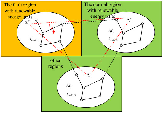
Figure 1.
Regional frequency spatiotemporal distribution.
AFR involves reasonably increasing feed-forward control based on the severity of a fault event. Units far from the disturbance node can act according to the parameters at the disturbance node. Taking the interconnected system in Figure 1 as an example, Δfi and tnadir,i represent the maximum frequency deviation and the time when the maximum frequency deviation occurs in each region, respectively. Each region participates in frequency regulation according to the frequency deviation command of Δf1 in the fault region, aiming to enable all units in the system to quickly and fully participate in frequency control. This approach is suitable for interconnected systems with obvious spatio-temporal distribution differences in frequency. A wide-area measurement system collects real-time data of key quantities. These include frequency, voltage, and power output. The data are centrally transmitted to the central control system. This enables real-time monitoring of the entire network status. It also allows for rapid adjustment of the network. When renewable energy sources participate, the operating information, such as unit information, power output, and control parameters, also needs to be collected. Through centralized communication methods, renewable energy units can exchange information with the system, enabling them to participate in active frequency response.
2.2. AFR Model of the Interconnected System in a Region with Renewable Energy Units
Taking the interconnected system in a region with renewable energy units as the research object, a frequency response model for it is constructed. The meanings of various parameters are shown in Appendix A, Table A1. In a region with renewable energy units, the power dynamic equation of the energy storage is shown in Equation (1).
The mechanical energy of the rotor of the wind turbine unit is transmitted to the gearbox through the low-speed shaft. After being speed-regulated by the gearbox, it is transmitted to the generator part through the high-speed shaft and converted into electrical energy. Wind turbines often employ a combined control strategy of torque and pitch angle. During normal operation, when the wind speed is within the range from low to the rated wind speed, to improve the utilization rate of wind energy, the system mainly relies on torque control. In combination with the maximum power tracking strategy, it precisely regulates the torque, enabling the wind turbine to track the wind speed and capture energy efficiently. Once the wind speed exceeds the rated value, the excessively high wind speed poses a threat to the safety and stability of the wind turbine. At this time, pitch angle control becomes crucial. By adjusting the pitch angle, the wind-facing angle of the blades is changed, thus limiting the energy absorption, controlling the power output, reducing the load on components, and ensuring the safe operation of the wind turbine under adverse wind conditions. Let the pitch angle Δβ and the torque ΔTg of the wind turbine generator be the control variables u2,i and u3,i. The dynamic equation of the wind power output is shown in Equation (2).
In the photovoltaic system, the direct current output by the photovoltaic array is boosted by a DC/DC converter and then serves as the DC power supply for the inverter. In the equivalent circuit, the photovoltaic array is connected to the inductor Ldc,i and the capacitor Cpv,i. By controlling the voltage duty cycle Δαi, the photovoltaic output voltage Udc,i can be adjusted, thereby controlling the output power. Taking the voltage duty cycle Δαi as the control variable u4,i, the power dynamic equation of the photovoltaic system is shown in Equation (3).
The specific control equations for thermal power units and hydroelectric power units, as well as the AFR control method, are presented in ref. [8], so they are not repeated here. The dynamic equation of the AC tie-line power is shown in Equation (4).
The frequency control equation of a region with renewable energy units is shown in Equation (5).
Among them, di represents the fluctuating power of renewable energy, and ΔPL,i represents the disturbance power caused by events. By performing the Laplace transform on the above power equations, the transfer function block diagram of the regional frequency response model for the high-proportion renewable energy system in Figure 2 can be obtained.
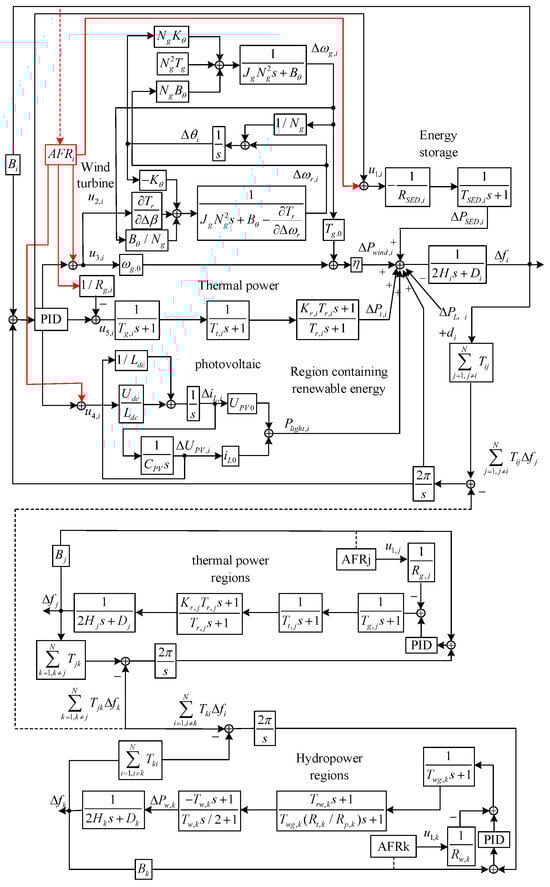
Figure 2.
AFR model of regional interconnection system with renewable energy.
To transform the regional model with renewable energy sources described in Figure 2 into a state-space model in the time domain, the state equation of region i with renewable energy sources is obtained as shown in Equation (6).
where xi is the state variable, ui is the control variable, and wi is the disturbance variable, and their elements are shown in Equations (7)–(9). Ai, Bi, Fi, and Ci are the state matrix, control matrix, disturbance matrix, and output matrix corresponding to the variables of a region i with renewable energy sources. The elements of Ci change with the variation in the AFR control objective, and the elements of Ai, Bi, and Fi correspond to Equations (1)–(5).
2.3. Ideas for Renewable Energy Participation in AFR
During normal system operation, renewable energy units operate with deloading and adjust their power output up and down to enable frequency response capabilities [19,20]. Wide-area communication is used to obtain the basic parameter information and real-time control parameters of each renewable energy unit, and then their power output and output range are determined to identify the available frequency regulation capacity. When participating in feed-forward control, the units adjust the output by regulating the parameter ui to respond to AFR commands.
As shown in Equation (5), to ensure regional stability, Δfi needs to be within a certain range. During the AFR process, the units receive signals to adjust ui and control the power output, providing full-force power support to the faulty area, which causes frequency fluctuations. If di is too large at this time, the remaining adjustment capacity of the units is insufficient to fully address the power fluctuations. In addition, for renewable energy sources to participate in AFR, sufficient power reserves need to be maintained according to system requirements. In response to the above two issues, the idea for renewable energy to participate in AFR are presented as shown in Figure 3.
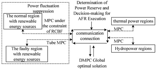
Figure 3.
The idea of renewable energy participating in AFR.
In traditional interconnected systems, the AFR is controlled using DMPC [8], that is, each sub-region solves its own MPC objective, and then a global optimization is carried out. Regions with renewable energy sources face power fluctuations. To handle this, we consider the control requirements of AFR. We use Tube and RCBF constraints to improve the DMPC. This forms a control method suitable for both conventional and renewable energy units. Moreover, an optimal power reserve link for renewable energy is added to the AFR decision-making process so that renewable energy sources can reserve sufficient power to implement the proposed control method.
3. AFR Control Method for Regions with Renewable Energy Based on Tube and RCBF Constraints
3.1. Tube MPC
The control principle of Tube MPC is shown in Figure 4. Tube MPC consists of two cascaded MPCs. The inner MPC control defines the reference trajectory using the traditional predictive control method with strict constraints. The outer MPC guides the state of the uncertain system towards the reference trajectory to form the actual trajectory. Therefore, over the entire optimization time domain, the actual trajectory of the system is always constrained within a “tube”.
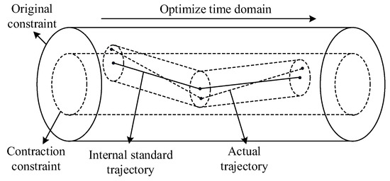
Figure 4.
Tube MPC control principle.
Then, ignoring the uncertain disturbances of the renewable energy, the inner-layer model of region i with renewable energy sources is described as:
The state variables and control variables are the same as those in the outer-layer model, but the disturbance variable and the disturbance matrix are modified as follows:
The objective of the inner-layer controller for region i with renewable energy sources is to achieve optimization while ignoring uncertain disturbances. Therefore, the objective function and the constraint conditions can be expressed as:
where Np is the prediction time domain, and Nc is the control time domain. , , , , γi, and γj are the weight matrices and weight coefficients of the inner MPC controller. At each sampling instant k, the inner-layer optimization problem is solved. and are the shrunk control variable constraint set and state variable constraint set, respectively.
To solve the above optimization problem, after obtaining the optimal solution (i,opt,i,opt), it should be transmitted to the outer-layer auxiliary MPC controller. During the process of tracking this optimal solution, the impact caused by the power fluctuations of renewable energy must be minimized. At this time, the objective function and constraint conditions of the outer-layer controller can be expressed as:
where Qi and Ri are the weight matrices of the outer MPC controller, Xi is the state variable constraint set, and Ui is the control variable constraint set.
Adopting the tube MPC algorithm for regions with renewable energy sources can reduce the instability of the power output of renewable energy sources, improve the control effect of AFR, and prevent the occurrence of frequencies exceeding the limit due to power fluctuations during the control process.
3.2. Constraints on the Control Parameters of Renewable Energy Sources Based on the RCBF
When solving the MPC for a region with renewable energy sources, the RCBF is used to constrain the control parameters of renewable energy sources to cope with power fluctuations. RCBF is a concept in control theory. It introduces safety constraints to prevent a system with uncertain disturbances from approaching dangerous areas or exceeding safety limits during its operation. According to Definition 3 in Ref. [21], let a continuously differentiable function be the RCBF. If there exists an extended class-K function αΘ that satisfies the Lipschitz continuity condition, is strictly increasing, and has an initial value of 0 (αΘ can be a proportional function), then the control system satisfies:
Then, the control system can satisfy the constraints under uncertain disturbances.
Suppose that the power disturbance range of a region i containing renewable energy sources is −di,max ≤ di ≤ di,max, and the maximum frequency safety deviation is Δfi,max, that is, −Δfi,max ≤ Δfi ≤ Δfi,max. Thus, the frequency safety constraints are formed as follows.
Given the power output equation and the frequency safety constraints, when hA(x) is taken as the RCBF and discrete processing is carried out, the system represented by Equation (6) should satisfy:
0 ≤ rA ≤ 1. The power output constraint equation of the renewable energy unit is:
If the changes in the power output of thermal power units with low capacity are not taken into account, then the constraint equations for the power increments of energy storage, wind power, and photovoltaic power can be obtained:
Among them, E, W, and L represent the capacity proportions of energy storage, wind power, and photovoltaic power. The same method can be used to construct the auxiliary RCBFs for Equations (20)–(22):
hAE(x), hAW(x) and hAL(x) should satisfy Equation (17). The same method can be used to obtain the control constraint of the energy storage that satisfies the positive frequency deviation:
Similarly, in the case of negative frequency deviation, it can be concluded that:
Similarly, the constraints on the control parameters u2,i, u3,I, and u4,i of the wind turbines and photovoltaic systems can be obtained. For details, refer to Equations (A1)–(A9) in Appendix B.
Thus, it can be seen that in each step of the MPC execution, the upper and lower limits of the control parameters that satisfy the RCBF will be formed. During the execution process, the restrictions on the control parameters of renewable energy sources can meet the frequency safety constraints and reduce the impact of power fluctuations.
3.3. The Improved DMPC Considering Power Fluctuations
Tube MPC is a very effective control method to deal with uncertain disturbances. However, it requires solving the objective function twice, which is not conducive to rapid solution. MPC with RCBF control parameter constraints can ensure frequency safety under power fluctuations, but it restricts power output and is not conducive to maximizing the provision of frequency-regulation resources. To meet the actual AFR requirements, a renewable energy AFR control method based on tube and RCBF constraints is formed.
When a fault occurs in a region with renewable energy sources, the units are required to provide as much power as possible. Therefore, tube MPC is adopted for the renewable energy units in a region with renewable energy sources to cope with power fluctuations. Regions with renewable energy sources can provide power support to other fault-affected regions. To speed up the solution of the overall algorithm, we take action. For renewable energy units in these regions, we adopt MPC under RCBF conditions. This helps deal with power fluctuations.
By combining tube and RCBF constraints, an improved DMPC method is formed. The steps are as follows:
- (1)
- Each sub-region assigns an initial solution u0 and an initial state x0 and transmits them to other regions.
- (2)
- Information from other regions and the predicted control sequence are received.
- (3)
- Each region solves the above-mentioned principle to obtain the control variable uk and the state variable xk at the current moment.
- (4)
- Each region transmits the predicted control sequence starting from the current moment and the state variable xk to other regions.
- (5)
- Control is implemented according to the currently solved control variable uk, followed by a return to Step 2.
We can use tube and RCBF constraints to suppress power fluctuations. Then, we can implement DMPC in combination with other conventional unit regions. This approach has multiple benefits. It reduces the solution time and meets the actual AFR requirements. Also, it lessens the impact of renewable energy power fluctuations.
4. AFR Decision Making Considering the Power Reserve of Renewable Energy Sources
In a system containing renewable energy sources, it is necessary to determine the optimal deloading rate of renewable energy units to ensure that the system has sufficient power reserves and guarantee the feasibility of renewable energy participation in the AFR. Aiming at the problem of determining the optimal deloading rate of renewable energy sources, this paper constructs an improved AFR control framework based on the principle of “online budgeting and real-time matching”, and the specific process is shown in Figure 5.
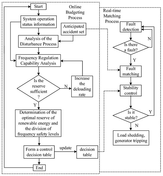
Figure 5.
Control decision for determining the optimal load reduction rate of renewable energy.
Online budgeting sets the control period for rolling optimization as 2 to 5 min. Under the established operation mode, only the set of anticipated accidents is analyzed for specific working conditions, and the decision-making table is updated. Given that the rolling period is relatively short, at the minute level, it can be assumed that the operating status of each control element remains unchanged.
First, we must obtain the actual output power of the units, the actual deloading rate of renewable energy sources, etc., and conduct online monitoring of the system operation parameters. In order to ensure the benefits of renewable energy farms and the economic efficiency of the system, conventional units are generally given priority for frequency regulation. Therefore, the adjustable reserve of conventional units in the system and the units that can participate in the regulation first must be calculated.
Under the anticipated accident scenario, it is assumed that the frequency response reserve of each conventional generator unit in the system is sufficient, and the quasi-steady-state frequency is quickly estimated. There is an approximate proportional relationship between the quasi-steady-state frequency Δfss and the maximum frequency deviation Δfmax [22]. In this paper, this conclusion is used to determine the frequency safety level and further derive the specific control strategy.
After quickly estimating Δfss offline under the anticipated accident scenario, an analysis of the system’s frequency regulation capability must be conducted. The power shortage and the power output increment of conventional units are:
where NT represents the number of conventional generator units; Rj is the frequency droop coefficient of the unit; ΔPup,j is the frequency response reserve of the unit; Pmax,j is the maximum output power of the unit; and Pj is the actual output power of the unit. If Δfss/Rj > ΔPup,j occurs, it indicates that the actual power shortage is greater than the power reserve of the conventional units, and renewable energy units need to adjust their output to make up for the power shortage. Thus, the power reserve of renewable energy required by the system is determined to adjust the deloading rate. If the reserve is insufficient, then the deloading rate needs to be increased to boost the power reserve of renewable energy. The frequency safety levels are classified according to the maximum frequency deviation Δfmax to decide whether renewable energy units will participate in the AFR.
The zoning of Δfmax is shown in Figure 6. fLD is the critical frequency of the dead zone, fLA is the critical frequency for auxiliary regulation, and fLE is the critical frequency of the emergency regulation zone. When Δfmax < fLA, the system is regarded as being in a normal operation state, and each unit can deal with it by using feedback control. When Δfmax > fLA, the system is regarded as being in a fault state. In order to prevent the maximum frequency deviation from exceeding the threshold, conventional units and renewable energy units implement AFR, and additional support from energy storage is required when the fault is severe. By combining with the aggregated analysis in the offline scenario, the specific control strategy of AFR is obtained, and the practical application of the AFR control method for renewable energy is realized.
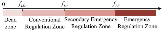
Figure 6.
Frequency safety level classification.
5. Calculation Examples
To verify the effectiveness and feasibility of the proposed AFR control method for renewable energy in a region with a high proportion of renewable energy, modeling and simulation are carried out on a three-area interconnected system. The advantages of renewable energy participating in AFR control using the control method proposed in this paper are analyzed and compared.
In MATLAB 2020a/simulink, a three-region interconnected power system as shown in Figure 2 is built to conduct a simulation study on the participation of renewable energy units in AFR. In the simulation system, the installed capacity ratio of the thermal-power area, the hydropower area, and the renewable energy area is 3:2:2. In the renewable energy area, the proportion of renewable energy is 80%, and the ratio of wind power, photovoltaic power, and energy storage is 6:3:1. The control equations for thermal power and hydropower can be found in Ref. [8], and the specific parameters of the system are shown in Table A2, Table A3 and Table A4 of Appendix A.
5.1. Determination of Renewable Energy Power Reserve
There are 10 adjustable conventional units in the thermal power area. If one of the units trips due to a fault, a power shortage of 950 MW will occur. The system follows the N-1 principle after an accident, that is, the system remains stable after tripping. After calculation, the maximum frequency deviation exceeds the set critical frequency for auxiliary regulation of 0.3 Hz, reaching 0.351 Hz. Therefore, it is necessary to use the renewable energy area for power support. If the hydropower area is not considered, the results of power shortage distribution and the required power reserve of renewable energy are shown in Figure 7.
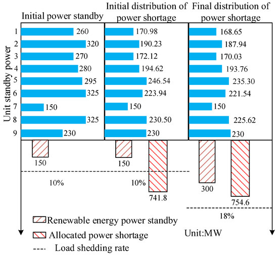
Figure 7.
Power allocation between thermal power units and renewable energy units.
After the fault, the power shortage of the system is distributed according to the unit regulation power of each generator unit. At this time, the renewable energy area operates with a deloading rate of 10%, and the power reserve is 150 MW. When the distribution starts, there is still a power shortage of 208.2 MW in the system. Moreover, Unit 7 and Unit 9 are already at full load and have lost their frequency response capability. Therefore, power support from renewable energy units is required, and the deloading rate is adjusted to 18%, with a power reserve of 300 MW. Then, theoretically, the renewable energy has sufficient power standby and can execute the AFR.
In the simulation of this paper, the capacity of the energy storage is only 50 MW, which obviously cannot meet the requirements for power reserve. In actual situations, after a system with a high proportion of renewable energy is disturbed, the power shortage required by the system is often relatively large, while the capacity of the energy storage is quite limited. Therefore, it is very necessary to reasonably control the renewable energy to provide a power reserve.
5.2. Verification of Tube MPC Algorithm
All the renewable energy units in the renewable energy area are affected by factors such as changes in wind speed and illumination, and they exhibit power fluctuations as shown in Figure 8.
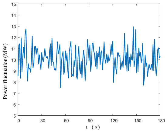
Figure 8.
The time-varying of di.
This subsection verifies the effectiveness of the tube MPC algorithm in suppressing power fluctuations. The area containing renewable energy is the area where disturbances occur; if a step disturbance occurs at 10 s, the resulting power shortage ΔPL,i is 1000 MW. The tube MPC algorithm in the area with new renewable energy participates in the optimization solution of the overall system. The prediction horizon of the DMPC algorithm in all sub-areas is set to 10, the control horizon is set to 3, and the sampling time is 0.1 s. The error weighting matrix and the control weighting matrix in the calculation objective function are diagonal matrices with 100 and 10 as diagonal elements, respectively, and the weight coefficients are γi = 0.7 and γj = 0.1.
The DMPC algorithm is compared with the DMPC algorithm proposed in this paper with the addition of the tube. The selection of the prediction horizon and the control horizon for the two algorithms is kept consistent. The frequency changes in each area are shown in Figure 9. When there is a power shortage, the frequency deviation with the addition of the tube is significantly reduced; that is, the power fluctuations of renewable energy have less impact on the system under control with the addition of the tube. This is because the tube MPC forms a frequency trajectory based on the power demand of the AFR, enabling the external controller to control the output of renewable energy units. Taking the standard trajectory as a reference, it forms a frequency trajectory that resists power fluctuations. With the addition of tube control, the conventional units and renewable energy units within the system can be better coordinated to meet the AFR requirements under power fluctuations.
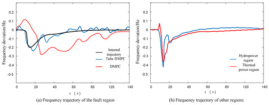
Figure 9.
Comparison of frequency response performance between DMPC with tube addition and DMPC.
The control signals of the renewable energy area in the power system under the two algorithms are shown in Figure 10. Compared with the DMPC algorithm with the addition of the tube, the changes and fluctuations in the control parameters of the conventional DMPC are significant. The reason is that the DMPC strategy needs to achieve two control objectives simultaneously: the delivery of AFR frequency regulation resources and the resistance to the power fluctuations of new energy. Therefore, during the optimization process, there is a trade-off in the optimization effects of the two control objectives.
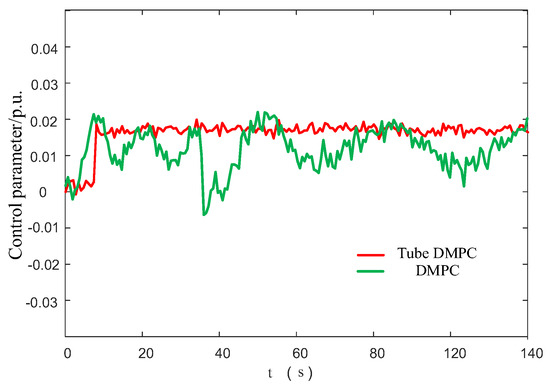
Figure 10.
Control signals for renewable energy regions.
We aim to further verify the superiority of the method proposed in this paper. To do so, we compare two aspects. First, we compare the control performance indicators. Second, we compare the average calculation time at each sampling moment. We compare these for the control algorithm proposed in this paper and the one adopting tube MPC in all areas. The results are shown in Table 1.

Table 1.
Comparison of algorithm performance.
Among them, the root mean square error of the frequency deviation is used as the performance indicator:
Stop represents the simulation step size. From the data in the table, it can be concluded that the algorithm proposed in this paper is slightly inferior to the control algorithm with Tube MPC adopted in all areas in terms of the effect of preventing frequency drops. However, it can ensure that the threshold is not breached, and the calculation time is significantly shortened. This is because in the method proposed in this paper, only the new energy units in the renewable energy fault area implement tube MPC control, and the units in other areas adopt MPC control. The tube DMPC needs to solve the optimization problem twice, which takes a long time. Therefore, the method proposed in this paper can meet the requirements of real-time optimization.
5.3. Verification of the Limiting Effect of RCBF Control Parameters
This subsection verifies the impact of the parameter limits of renewable energy units in the RCBF on the results of the MPC algorithm when the renewable energy region is regarded as a normal region. A severe fault occurs in the thermal power region, leading to the disconnection of large-capacity units, and power shortage ΔPL,i remains at 1000 MW. All sub-regions also adopt the DMPC (distributed model predictive control) algorithm. During the execution of the algorithm, the results of the RCBF constraints are calculated by obtaining the changes in the power output of renewable energy sources and are restricted by the control parameters.
As can be seen from Figure 11, after a disturbance occurs in the thermal power region, the units in the renewable energy region provide power support, but the frequency within the region also begins to drop. Judging from the comparison results, the frequency control effect under the constraint of RCBF is better. The most significant difference between the cases with and without the RCBF constraint lies in the maximum frequency deviation of the region and the time when it is reached. Under the constraint of the RCBF control parameters, the maximum frequency deviation of the frequency is significantly reduced, and the time of its occurrence is also extended. This is because the renewable energy units force the system to meet specific frequency constraint conditions during the control process in response to the AFR frequency regulation requirements. This can ensure that the system state will not violate the pre-set safety boundaries under any circumstances. Even in the presence of uncertainties, it can adjust the control input to keep the system within the safe area. Therefore, the limitation of the parameters of the renewable energy units retains the prevention against the maximum power fluctuations. When there is no RCBF constraint, the power fluctuations intensify the impact of system disturbances, increasing the maximum frequency deviation, the maximum frequency deviation has a faster arrival time, and posing a greater risk to the safety of the system frequency.
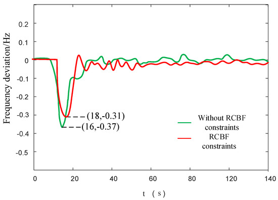
Figure 11.
Frequency change in the renewable energy region.
As can be seen from Figure 12, under AFR control, each renewable energy unit promptly increases its power output to prevent the frequency drop in its local region. Moreover, under the limitation of the new RCBF energy control parameters, the new energy units can limit the impact of power fluctuations when participating in AFR and can provide power to the maximum extent. Among them, the energy storage reaches the power upper limit and maintains the maximum output.
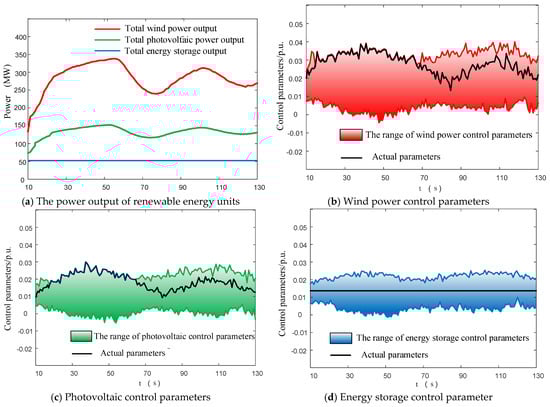
Figure 12.
Renewable energy output and control parameters.
6. Conclusions
This paper proposes a control method for the AFR of renewable energy units based on tube MPC and RCBF constraints and takes into account the power reserve of renewable energy. The correctness and effectiveness of the proposed method are analyzed and verified through a three-area interconnected power system model. The simulation analysis shows that:
- (1)
- When a fault occurs in a region with renewable energy, aiming at the adverse impact of power fluctuations on the control when renewable energy participates in AFR control, a control algorithm of tube MPC is proposed. This algorithm enables renewable energy units in the fault region of renewable energy to cope with the uncertain fluctuations of renewable energy. At the same time, the DMPC algorithm is applied to the units in other areas. The simulation shows that this method can achieve real-time optimization of the overall system and improve the control accuracy. Faults may occur in regions of conventional units. When this happens, renewable energy units in renewable energy regions can take action. They reduce the impact of uncertain renewable energy fluctuations. They do this while meeting the constraints of RCBF control parameters. This endows these units with AFR capability. As a result, it ensures the frequency stability of the local region and provides frequency regulation resources.
- (2)
- We add the optimal deloading operation mode of renewable energy units to the link of online generation of AFR control decisions. This ensures renewable energy has sufficient power reserves when it participates in AFR. As a result, renewable energy can smoothly participate in AFR.
Author Contributions
Conceptualization, X.D.; methodology, C.C.; investigation, C.C.; resources, C.C.; data curation, C.C.; writing—original draft preparation, X.D.; writing—review and editing, C.C.; visualization, X.D.; supervision, X.D. All authors have read and agreed to the published version of the manuscript.
Funding
This research was funded by Science and Technology Project Funding from China Southern Power Grid Corporation (CGYKJXM20220115).
Data Availability Statement
Data are contained within the article. The data presented in this study are available in the cited references.
Conflicts of Interest
The authors declare no conflicts of interest.
Abbreviations
The following abbreviations are used in this manuscript:
| MDPI | Multidisciplinary Digital Publishing Institute |
| DOAJ | Directory of open access journals |
| TLA | Three-letter acronym |
| LD | Linear dichroism |
Appendix A
Table A1.
Variables and physical meanings.
Table A1.
Variables and physical meanings.
| Variable | Physical Meaning | Variable | Physical Meaning |
|---|---|---|---|
| TSED,i | Energy storage delay response coefficient | PSED,i | Energy storage power |
| RSED,i | Energy storage sag coefficient | u1,i | Energy storage control parameters |
| Tr,i | Wind turbine torque | Ng,i | Gearbox transmission ratio |
| Jr,i | Low-speed shaft moment of inertia | Jg,i | High-speed shaft moment of inertia |
| ωr,i | Wind turbine rotor speed | ωg,i | Wind turbine speed |
| Kθ,i | Stiffness | θi | Transmission shaft torsion angle |
| Bθ,i | Damping coefficient | Tg,i | Wind turbine torque |
| βi | Pitch angle | Pwind,i | Wind turbine output power |
| Ldc,i | Photovoltaic inductor | iL,i | Photovoltaic output current |
| UPV,i | Photovoltaic array output voltage | CPV,i | Photovoltaic capacitor |
| Udc,i | Photovoltaic output voltage | Plight,i | Photovoltaic output power |
| Rg,i | Adjustment coefficient of thermal power unit in region i | Tg,i | Time constant of turbine governor in region i |
| Tr,i | Reheat time constant of steam turbine in region i | Kr,i | Coefficient of reheat turbine in region i |
| Pt,i | Output power of thermal power units in region i | Δfi | Frequency deviation in region i |
| Hi | Equivalent inertia time constant of region i | Di | Equivalent load damping coefficient of region i |
| Bi | Frequency deviation coefficient of region i | Tij | Power synchronization coefficient for regions i and j |
| Δfj | Frequency deviation of region j | Hj | Equivalent inertia time constant of region j |
| Dj | Equivalent load damping coefficient of region j | Rg,j | Region J thermal power unit adjustment coefficient |
| Tg,j | Time constant of turbine governor in region j | Tr,j | Reheating time constant of steam turbine in region j |
| Kr,j | Coefficient of reheating turbine in region j | Pt,j | Output power of thermal power units in region j |
| Bj | Frequency deviation coefficient of region j | Tjk | Power synchronization coefficient for regions j and k |
| Δfk | Frequency deviation of region k | Hk | Equivalent inertia time constant of region k |
| Dk | Equivalent load damping coefficient of region k | Rw,k | Adjustment coefficient of water turbine |
| Twg,k | Time constant of turbine governor | Trw,k | Reset time constant of turbine governor |
| Tw,k | Turbine time constant | Rp,k | Temporary decrease rate of turbine governor |
| Rt,k | Permanent descent rate of turbine governor | Pw,k | Output power of hydroelectric units |
| Bk | Frequency deviation coefficient of region k |
Table A2.
Parameters of renewable energy region.
Table A2.
Parameters of renewable energy region.
| Variable | Parameter | Variable | Parameter |
|---|---|---|---|
| H | 6 | D | 1 |
| RSED | 1 | TSED | 0.1 |
| Ng | 100:1 | ωr | 12 |
| ωg | 1200 | Tg | 43,000 |
| Jr | 0.5 | Jg | 0.5 |
| Kθ | 2 | Bθ | 0.25 |
| Ldc | 0.001 | CPV | 0.004 |
| Rg | 1 | Tg | 0.1 |
| Tr | 0.3 | Kr | 12 |
| Tij | 0.5 | B | 20 |
Table A3.
Parameters of thermal power region.
Table A3.
Parameters of thermal power region.
| Variable | Parameter | Variable | Parameter |
|---|---|---|---|
| H | 18 | D | 3 |
| Rg | 0.042 | Tg | 0.1 |
| Tr | 0.3 | Kr | 12 |
| B | 40 | Tjk | 0.5 |
Table A4.
Parameters of hydropower region.
Table A4.
Parameters of hydropower region.
| Variable | Parameter | Variable | Parameter |
|---|---|---|---|
| H | 6 | D | 1 |
| Rw | 0.125 | Twg | 0.1 |
| Trw | 5 | Tw | 5 |
| Rp | 0.05 | Rt | 1 |
| B | 30 |
Appendix B
Constraints on the control parameters of wind turbine units:
Constraints on the control parameters of photovoltaic systems:
References
- Han, Z.; Ju, P.; Qin, C.; Sun, D.; Sun, H.; Zheng, Y. Review and prospect of research on frequency security of renewable power system. Electr. Power Autom. Equip. 2023, 43, 112–124. [Google Scholar]
- Han, L.; Xu, G.; Wang, C.; Bi, T. Correlation Analysis and Distribution Characterization of Frequency Regulation Resources and Frequency Spatiotemporal Dynamics in Renewable Energy Power Systems. Proc. CSEE 2024, 1, 0258–8013. [Google Scholar]
- Li, M.; Chang, Y.; Mao, Y.; Liu, E.; Wang, X.; Zhang, X.; Geng, H. Review and Prospect of Stability Control Techniques for Grid-following Grid-forming Converters in High-penetration Renewable Energy Generation. High Volt. Eng. 2024, 50, 4773–4788. [Google Scholar]
- Yan, K.; Li, G.; Zhang, R.; Xu, Y.; Jiang, T.; Li, X. Frequency Control and Optimal Operation of Low-Inertia Power Systems with HVDC and Renewable Energy: A Review. IEEE Trans. Power Syst. 2024, 39, 279–4295. [Google Scholar] [CrossRef]
- Zhang, Z.; Kou, P.; Zhang, Y.; Liang, D. Coordinated Predictive Control of Offshore DC Collection Grid and Wind Turbines for Frequency Response: A Scheme without secondary Frequency Drop. IEEE Trans. Sustain. Energy 2023, 14, 1488–1503. [Google Scholar] [CrossRef]
- Harandi, M.; Bina, M.; Golkar, M.; Harandi, M.; Toulabi, M. Inertial Frequency Response of Wind Turbines Using Adaptive Full Feedback Linearization Control: Stability and Robustness Analysis. IEEE Trans. Sustain. Energy 2024, 15, 2777–2788. [Google Scholar] [CrossRef]
- Yan, C.; Yao, W.; Wen, J. Impact of Active Frequency Support Control of Photovoltaic on PLL-Based Photovoltaic of Wind-Photovoltaic-Thermal Coupling System. IEEE Trans. Power Syst. 2023, 38, 4788–4799. [Google Scholar] [CrossRef]
- Li, W.; Jin, C.; Wen, K.; Shen, J.; Liu, J. Active Frequency Response Control Under High-power Loss. Autom. Electr. Power Syst. 2018, 42, 22–30. [Google Scholar]
- Jin, C.; Li, W.; Shen, J.; Li, P.; Liu, L.; Wen, K. Active frequency response based on model predictive control for bulk power system. IEEE Trans. Power Syst. 2019, 34, 3002–3013. [Google Scholar] [CrossRef]
- Wu, X.; Li, Z.; Li, W.; Jin, C. An Active Frequency Response Control Strategy for Back-to-back DC Interconnection System. High Volt. Eng. 2022, 48, 1003–6520. [Google Scholar]
- Wu, X.; Li, W.; LI, Z.; Zhen, H.; Zeng, H.; Li, Z. Optimal Control Strategy of Active Frequency Response Against Large Disturbance Considering Electrochemical Energy Storage. Autom. Electr. Power Syst. 2023, 47, 118–127. [Google Scholar]
- Yang, D.; Zhu, J.; Jiang, C.; Hao, Z.; Zhao, G. Highly-proportional Wind Power System Multi-Source Collaborate Load Frequency Control Strategy Based on Distributed Model Prediction. Power Syst. Technol. 2024, 48, 2804–2814. [Google Scholar]
- Li, Z.; Bai, N.; Cheng, Z.; Wang, Y.; Sui, Q. Distributed Collaborative AGC Method for Heterogeneous Frequency Regulation Units in New Power Systems. Power Syst. Technol. 2024, 48, 2327–2335. [Google Scholar]
- Liu, X.; Wang, C.; Kong, X.; Zhang, Y.; Wang, W.; Lee, K.Y. Tube-Based Distributed MPC for Load Frequency Control of Power System with High Wind Power Penetration. IEEE Trans. Power Syst. 2024, 39, 3118–3129. [Google Scholar] [CrossRef]
- Qian, M.; Zhang, J.; Qin, W.; Yang, D.; Wang, X. System frequency response characteristic considering DFIG frequency regulation and fast frequency response strategy. Power Syst. Prot. Control 2025, 53, 58–67. [Google Scholar]
- Zhang, X.; Zhu, Y.; Fu, Y. Wind-storage Cooperative Fast Frequency Response Technology Based on System Inertia Demand. Proc. CSEE 2023, 43, 5415–5429. [Google Scholar]
- Liu, J.; Liu, X.; Liu, J.; Li, X.; Wang, J. Adaptive-Droop-Coefficient VSG Control for Cost Efficient Grid Frequency Support. IEEE Trans. Power Syst. 2024, 39, 6768–6771. [Google Scholar] [CrossRef]
- Qin, B.; Xu, Y.; Yuan, C.; Jia, J. A Unified Method of Frequency Oscillation Characteristic Analysis for Multi-VSG Grid-Connected System. IEEE Trans. Power Deliv. 2022, 37, 279–289. [Google Scholar] [CrossRef]
- Ge, X.; Han, Y.; Fu, Y.; Qian, J.; Zhu, H. Whole Prosess Frequency Correction Method of Wind Power High Proportion System Based on Differential Deloading Strategy. Power Syst. Technol. 2024, 48, 4958–4968. [Google Scholar]
- Zhong, L.; Xiong, J.; Zhang, X.; Yang, Z. A risk-reduction emergency control method of a power system based on photovoltaic power reserve. Power Syst. Prot. Control 2021, 49, 157–167. [Google Scholar]
- Josseph, B.; Dimitra, P. Robust Control Barrier Functions under high relative degree and input constraints for satellite trajectories. Automatica 2023, 155, 111109. [Google Scholar]
- Shen, J.; Li, W.; Liu, L.; Jin, C.; Wen, K.; Wang, X. Frequency Response Model and Its Closed-Form Solution of Two-Machine Equivalent Power System. IEEE Trans. Power Syst. 2021, 36, 2162–2173. [Google Scholar] [CrossRef]
Disclaimer/Publisher’s Note: The statements, opinions and data contained in all publications are solely those of the individual author(s) and contributor(s) and not of MDPI and/or the editor(s). MDPI and/or the editor(s) disclaim responsibility for any injury to people or property resulting from any ideas, methods, instructions or products referred to in the content. |
© 2025 by the authors. Licensee MDPI, Basel, Switzerland. This article is an open access article distributed under the terms and conditions of the Creative Commons Attribution (CC BY) license (https://creativecommons.org/licenses/by/4.0/).