Evaluation of the Impact of Multi-Scale Flow Mechanisms and Natural Fractures on the Pressure Transient Response in Fractured Tight Gas Reservoirs

Abstract

The coupling mechanism between the multi-scale flow mechanisms and the pressure dynamic response of complex fracture networks in fractured tight sandstone gas reservoirs remains unclear. In this study, a mathematical model was developed by incorporating the non-Darcy flow (non-DF) behavior in both matrix and fracture systems within the framework of the embedded discrete fracture model (EDFM). The governing equations were solved numerically through finite volume discretization. By employing numerical well-testing techniques, the dynamic impacts of low-velocity non-DF (matrix domain) and high-velocity non-DF (fracture domain) on the pressure transient response were systematically evaluated. Furthermore, the characteristic patterns of transient pressure responses under different natural fracture development modes were revealed. This study demonstrates that the pressure and pressure derivative (PD) log–log curves of fractured tight sandstone gas wells exhibit a wide opening shape, indicative of complex fracture morphologies. The presence of a threshold pressure gradient in the matrix system results in an upward convex shape in the PD profile, whereas the high-velocity non-DF in the fracture network causes a downward concave characteristic in the derivative curve. The spatial distribution of the natural fracture network significantly influences the response characteristics during the mid-term radial flow stage. As the fracture density decreases, the system gradually transitions toward a dual-porosity medium. This research contributes to the theoretical foundation required for the accurate interpretation of dynamic well tests and the optimization of effective development schemes in gas reservoirs with extremely low permeability.

1. Introduction

As conventional oil and gas resources become increasingly depleted, fractured tight sandstone gas reservoirs have emerged as a key focus area for global unconventional natural gas development [1,2]. These reservoirs are typically characterized by nano-scale pore-throat structures and complex natural fracture networks, exhibiting strong multi-scale nonlinear flow effects during development [3]. The presence of fine pore throats and natural fractures in these reservoirs results in flow mechanisms that significantly differ from those of conventional gas reservoirs [4], making it difficult to accurately describe their flow behavior and development characteristics using conventional methods.

Well-test analysis is a critical method for revealing reservoir characteristics and understanding gas reservoir production dynamics. It also serves as the foundation for formulating development plans and adjusting technical strategies for gas reservoirs [5]. In the analysis of well testing for fractured reservoirs, the Warren–Root model has gained predominant acceptance within the industry. This model characterizes the fluid exchange between fracture networks and rock matrices using two key parameters: ω (the elastic storativity ratio) and λ (the interporosity flow coefficient) [6]. However, the Warren–Root model is only suitable for carbonate reservoirs with relatively homogeneous natural fracture development. In contrast, fractured tight sandstone gas reservoirs often exhibit discrete and irregular medium-to-large-scale natural fractures, with significant variations in fracture length, aperture, and spacing [7,8]. Traditional dual-porosity, dual-permeability models struggle to accurately characterize the complex spatial configuration between natural and hydraulic fractures, particularly the influence of natural fracture spatial distribution patterns on pressure wave propagation, which requires further investigation [9,10]. In recent years, several researchers constructed an unconventional fracture model (UFM) to simulate the real-time growth of complex hydraulic–natural fracture networks [11], considering fluid flow, interactions between hydraulic and natural fractures, and reservoir petrophysics. Several scholars also proposed an EDFM, which uses unstructured grids to represent discrete fracture geometries and demonstrates unique advantages over other discrete fracture models in simulating complex fracture networks [12]. The EDFM has the ability to flexibly capture complex irregular crack geometries and is suitable for multi-scale distributed crack systems. It also enables efficient calculations and has a modular design, making it easy to expand and apply in engineering.

Furthermore, previous studies often simplify the flow in fracture systems as Darcy flow (DF) and focus on fracture network characterization under DF conditions. The coupling mechanism between low-velocity non-DF in the matrix and high-velocity non-DF in fractures has not been systematically examined, leading to the neglect of the impact of nonlinear flow on gas movement in reservoirs and resulting in significant deviations in well-testing dynamic analysis [13]. Nie [14] developed a radial dual-zone composite non-DF model based on the Izbash equation, confirming that non-DF significantly affects the pressure transient behavior of fractured reservoirs. Zhu [15] established a theoretical model considering the threshold pressure gradient, providing more accurate production predictions. Fu [16] proposed a multi-stage fractured horizontal well-productivity model with multi-scale flow mechanisms, which more accurately characterizes the flow behavior of fractured horizontal wells in tight sandstones. Geng [17] demonstrated that the pressure transient analysis model considering nonlinear flow mechanisms yields more accurate log–log pressure and PD curve fitting results. Extensive research has shown that nonlinear flow mechanisms in tight gas reservoirs have a significant impact on gas well-dynamic analysis. However, previous pressure transient analysis models for fractured tight sandstone gas reservoirs rarely consider the nonlinear flow mechanisms in both the matrix and fractures as well as the complex fracture distribution patterns.

In this study, an EDFM numerical model coupled with multi-scale non-DF mechanisms is proposed. In this model, the matrix system is described using a modified Darcy equation to account for the nonlinear flow influenced by the threshold pressure gradient, while the fracture system incorporates the Forchheimer equation to characterize high-velocity turbulent flow effects. By establishing a typical numerical model for fractured tight gas reservoirs and employing numerical well-testing techniques, the sensitivity of different flow mechanisms to the PD curve morphology is systematically analyzed. Additionally, the regulatory effects of the natural fracture density, connectivity, and spatial configuration on the transient response characteristics are investigated. This research breaks through the limitations of the “DF assumption” in traditional well-test analysis, providing a new theoretical model for the dynamic inversion of complex fractured gas reservoirs. Compared with the EDFM numerical model, this model significantly improves the simulation accuracy of the pressure transient response by comprehensively considering the multi-scale non-Darcy flow mechanism in the matrix and fractures. At the same time, the finite volume method and TPFA discretization scheme are used to greatly improve the computational efficiency while ensuring numerical stability. In addition, the modular design and general algorithm provide the model with good usability and portability, and it can be easily integrated into various engineering software platforms.

2. Methodology

2.1. Governing Equation

The mass conservation equation for fluid flow in the matrix is expressed as follows [12]:

$${\displaystyle \frac{\partial \left({\varphi }^m{\rho }_{\alpha }{S}_{\alpha }^m\right)}{\partial t}}+\nabla \cdot \left({\rho }_{\alpha }{\overrightarrow{u}}_{\alpha }^m\right)={\rho }_{\alpha }\left[q_{\alpha }^m-{\displaystyle \sum _{i=1}^{N_f}{q}_{\alpha }^{m,fi}}\right]$$

(1)

where m is the matrix; S is the saturation, decimal; t is the time, s; ϕ is the porosity, decimal; q^m,fi is the fluid exchange term between the matrix and fracture, (m³/s)/m²; α is the fluid phase, either gas or water; ${\overrightarrow{\mathit{u}}}^{\mathit{m}}$ is the velocity of the fluid in the matrix, m/s; ρ is the fluid density, kg/m³; ∇ is the divergence operator; ${\mathit{f}}_{\mathit{i}}$ is the fractures index.

The low-velocity non-DF in the matrix of tight reservoirs can be expressed as follows [17]:

$${\overrightarrow{u}}_{\alpha }^m=-{\displaystyle \frac{K{k}_{r\alpha }}{{\mu }_{\alpha }}}\eta \nabla p$$

(2)

where K is the permeability, m²; η is the low-velocity non-Darcy coefficient, which is dimensionless; μ_α is the fluid phase viscosity, Pa·s; k_rα is the relative permeability, decimal; ∇p is the pressure gradient, Pa/m.

The low-velocity non-Darcy coefficient η is calculated as follows [18]:

$$\eta =\left\{\begin{array}{l}0,\left|\nabla p\right|\le \lambda \\ {\left(1-{\displaystyle \frac{\lambda }{\left|\nabla p\right|}}\right)}^4\left(1-{\displaystyle \frac{4}{3}}{\displaystyle \frac{\delta -\lambda }{\left|\nabla p\right|-\lambda }}\right),\left|\nabla p\right|>\lambda \end{array}\right.$$

(3)

where λ is the starting pressure gradient, Pa/m.

The flow in fractures is described using Nf mass conservation equations, with each fracture represented by the index fi. The conservation equation for each fracture is given by the following:

$${\displaystyle \frac{\partial \left({\varphi }^{fi}{\rho }_{\alpha }{S}_{\alpha }^{fi}\right)}{\partial t}}+\nabla \cdot \left({\rho }_{\alpha }{\overrightarrow{u}}_{\alpha }^{fi}\right)={\rho }_{\alpha }\left[q_{\alpha }^{fi,w}+q_{\alpha }^{fi,m}+q_{\alpha }^{fi,fj}\right]$$

(4)

where ${\overrightarrow{\mathit{u}}}_{\mathit{\alpha }}^{{\mathit{f}}_{\mathit{i}}}$ is the fluid velocity in fracture, m/s; ${\mathit{q}}_{\mathit{\alpha }}^{{\mathit{f}}_{\mathit{i}},\mathit{w}}$ is the fluid exchange between fractures and wells, (m³/s)/m²; ${\mathit{q}}_{\mathit{\alpha }}^{{\mathit{f}}_{\mathit{i}},{\mathit{f}}_{\mathit{j}}}$ is the fluid exchange between fractures, (m³/s)/m²; ${\mathit{q}}_{\mathit{\alpha }}^{{\mathit{f}}_{\mathit{i}},\mathit{m}}$ is the fluid exchange between fractures and matrix, (m³/s)/m².

The hydrodynamic similarity criterion is a dimensionless combination of physical quantities that characterizes certain physical effects and ensures similarity between flows of different scales. The Reynolds number (R_e), as a similarity criterion in viscous flow, serves as a bridge between pore-scale flow and macroscopic flow in this study. A smaller Reynolds number indicates more significant viscous effects, while a larger Re indicates more significant inertial effects. The Reynolds number is expressed as follows:

$$R_e={\displaystyle \frac{{\rho }_{\alpha }{\overrightarrow{u}}_{\alpha }^{fi}d}{{\mu }_{\alpha }}}$$

(5)

where d is the characteristic length of fracture, m.

This study uses a critical Reynolds number model to determine the boundary between DF and high-velocity non-DF in fractures. The flow regime in fractures is determined by comparing the Reynolds number R_e with the critical Reynolds number R_ec. The critical Reynolds number model is expressed as follows:

$$R_{ec}={\displaystyle \frac{d}{\beta }}\left({\displaystyle \frac{1}{0.99k_D}}-{\displaystyle \frac{1}{k_D}}\right)={\displaystyle \frac{d}{99k_D\beta }}$$

(6)

where k_D is the Darcy permeability of fracture, m²; β is the non-Darcy coefficient, 1/m.

The characteristic length of the fracture is taken as the mechanical aperture of the fracture. For the Darcy permeability of propped hydraulic fractures, the predictive model established by [18] is used:

$$k_f=4.69\times {10}^{-6}{e}^{-{\displaystyle \frac{1.05}{a_f+0.18}}+2.54{\varphi }^2+3.40\varphi -7.68}\cdot s^{1.51}$$

(7)

where ϕ is the prop hydraulic fracture porosity, decimal; S is the proppant particle size, 10⁻³ m; a_f is the mechanical opening of the supporting hydraulic fracture, m.

For the Darcy permeability of rough natural fractures, the model proposed by [19] is adopted:

$$k_f={\displaystyle \frac{a_f^2}{12}}\cdot e^{-{\displaystyle \frac{0.75Z_2}{\sqrt{a_f}}}}$$

(8)

where Z₂ is the fracture roughness height variation coefficient, dimensionless; a_f is the mechanical aperture of rough natural fractures, m.

For the non-Darcy coefficient in hydraulic fractures, the model established by [20] is used:

$$\beta ={\displaystyle \frac{408}{a^{0.3667}{s}^{0.7601}{\varphi }^{4.4369}}}$$

(9)

For the non-Darcy coefficient in natural fractures, the model established by [21] is applied:

$$\beta =2.7606e^{0.0872a_f+{\displaystyle \frac{2.2809}{JR{C}^{3D}+0.5453}}}$$

(10)

When the Reynolds number of the flow is less than the critical Reynolds number Rec, the flow in the fracture is DF, modeled by Darcy’s law:

$${\overrightarrow{u}}_{\alpha }^{fi}=-{\displaystyle \frac{\mathit{K}{k}_{r\alpha }}{{\mu }_{\alpha }}}\nabla p_{fi}$$

(11)

When the Reynolds number of the flow exceeds the critical Reynolds number Rec, the flow in the fracture is high-velocity non-DF. The high-velocity non-DF caused by turbulence and inertial effects is calculated using the Forchheimer equation [22]:

$$-\nabla p_{fi}={\displaystyle \frac{{\mu }_{\alpha }}{\mathit{K}{k}_{r\alpha }}}{\overrightarrow{u}}_{\alpha }^{fi}+{\rho }_{\alpha }\beta {\left({\overrightarrow{u}}_{\alpha }^{fi}\right)}^2$$

(12)

Note: The model in this paper does not consider coupling with energy balance. This is because the study focuses on the impact of multi-scale non-Darcy flow mechanisms on pressure transient response in tight gas reservoirs. Under the target reservoir conditions, the temperature change is relatively small. Therefore, the isothermal assumption can simplify the model while focusing on the fluid dynamics process and ensuring the stability and efficiency of the numerical solution. In cases with large thermal gradients or future extended studies, it will be a very valuable research direction to consider the free convection effect by combining energy conservation with momentum balance [23].

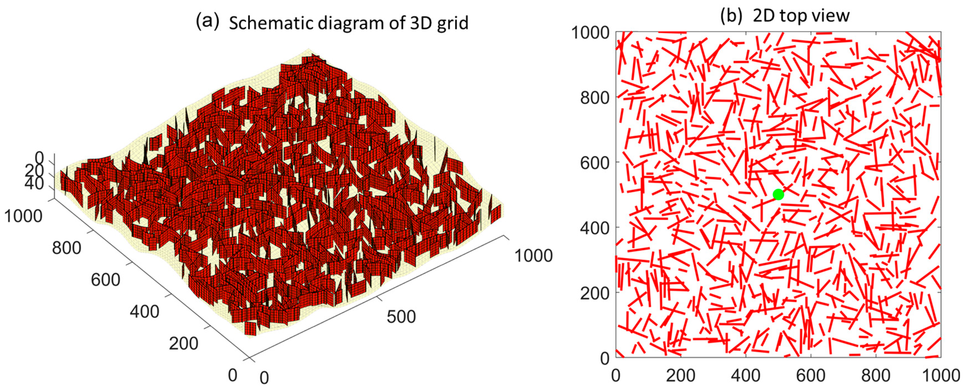
2.2. Numerical Model and Solutions

Within the framework of the finite volume methodology, the embedded discrete fracture model is formulated, with the governing equations being numerically solved through discrete approximation based on the same numerical approach [24]. The fluid flow component in the governing Equation (1) can be mathematically represented through the following discretization scheme:

$$\nabla \cdot \left({\rho }_{\alpha }{\overrightarrow{u}}_{\alpha }^m\right)=\sum _j{\rho }_{\alpha }{\lambda }_{\alpha }{T}_{ij}^{mm}\left(p_{\alpha }^i-p_{\alpha }^j\right)$$

(13)

where ${\mathit{p}}_{\mathit{\alpha }}^{\mathit{i}}$ is the fluid pressure of phase α in grid i, Pa; ${\mathit{p}}_{\mathit{\alpha }}^{\mathit{j}}$ is the fluid pressure of phase α in grid j, Pa; λ_α is the upwind weighted flow of phase α, m²/(Pa·s).

${\mathit{T}}_{\mathit{i}\mathit{j}}^{\mathit{m}\mathit{m}}$ is the nonlinear conductivity with upwind weighting between two matrix grids:

$$T_{ij}^{mm}={\displaystyle \frac{T_{i,j}\cdot T_{j,i}}{T_{i,j}+T_{j,i}}}\cdot \eta$$

(14)

The unilateral conductivity ${\mathit{T}}_{\mathit{i},\mathit{j}}$ associated with grid i is calculated by the following equation:

$$T_{i,j}={\displaystyle \frac{A_{i,j}{K}_i^m{\overrightarrow{c}}_{i,j}\cdot {\overrightarrow{n}}_{i,j}}{{\left|{\overrightarrow{c}}_{i,j}\right|}^2}}$$

(15)

when the matrix grid ${\mathit{\Omega }}_{\mathit{i}}$ intersects with the fracture grid ${\mathit{\psi }}_{\mathit{i}}$, the fluid exchange term ${\mathit{q}}_{\mathit{\alpha }}^{\mathit{m},\mathit{f}}$ between each matrix and fracture grid is discretized using the TPFA (total pressure-based finite volume approximation) method as follows:

$$q_{\alpha }^{m,f}=T^{mf}{\lambda }_{\alpha }\left(p_{\alpha }^m-p_{\alpha }^f\right)$$

(16)

where ${\mathit{T}}^{\mathit{m}\mathit{f}}$ is the conductivity between matrix grid and fracture grid, m³; ${\mathit{p}}_{\mathit{\alpha }}^{\mathit{m}}$ is the matrix grid pressure, Pa; ${\mathit{p}}_{\mathit{\alpha }}^{\mathit{f}}$ is the pressure of the fracture grid, Pa.

The flow term in the governing Equation (4) can be discretized as follows:

$$\nabla \cdot \left({\rho }_{\alpha }{\overrightarrow{u}}_{\alpha }^{f_i,ND}\right)=\sum _j{\rho }_{\alpha }{\lambda }_{\alpha }{T}_{ij}^{ff}\left(p_{\alpha ,i}^f-p_{\alpha ,j}^f\right)$$

(17)

${\mathit{T}}_{\mathit{i}\mathit{j}}^{\mathit{f}\mathit{f}}$ is the corrected conductivity between fracture grids:

$$T_{ij}^{ff}={\displaystyle \frac{T_i^f{T}_j^f}{T_i^f+T_j^f}}\cdot F_{ND}$$

(18)

where F_ND is the high-velocity non-DF factor, defined as follows [25]:

$$F_{ND}={\displaystyle \frac{2}{1+\sqrt{1+\frac{4{\rho }_{\alpha }{\beta }_{\alpha }{K}^f{k}_{r\alpha }}{{\mu }_{\alpha }}\cdot \frac{K^f{k}_{r\alpha }}{{\mu }_{\alpha }}\nabla p^f}}}$$

(19)

when two fractures f_i and f_j intersect, the fluid exchange term at the fracture junction is still discretized using the two-point flux approximation:

$$q_{\alpha }^{f_i,f_j}=T_{f_i{f}_j}^{ff}{\lambda }_{\alpha }\left(p_{\alpha }^{f_j}-p_{\alpha }^{f_i}\right)$$

(20)

${\mathit{T}}_{{\mathit{f}}_{\mathit{i}}{\mathit{f}}_{\mathit{j}}}^{\mathit{f}\mathit{f}}$ represents the harmonic average conductivity between fractures f_i and f_j, calculated as follows:

$$T_{f_i{f}_j}^{ff}={\displaystyle \frac{T^{f_i}{T}^{f_j}}{T^{f_i}+T^{f_j}}}\cdot F_{ND}$$

(21)

Compared to the flow resistance between grids, the flow resistance effect caused by high-velocity non-DF around the wellbore is much greater. The impact of high-velocity non-DF on well production can be represented by a rate-dependent skin factor. The well index in this case is written as follows:

$$W{I}^f={\displaystyle \frac{2\pi k^f{a}^f}{\ln \left(r_e/r_w\right)+s_0+D_{\alpha }q}}$$

(22)

where s₀ is the mechanical skin factor, and D_αq is the rate-dependent skin factor generated by high-velocity non-DF.

2.3. Evaluation of Pressure and PD Evaluation

In the pressure log–log curve, there are often two curves: one is the pressure difference (DP) vs. time log–log curve, and the other is the pressure difference derivative (DPP) vs. time log–log curve. The DP is calculated as follows:

$$\Delta p\left(t\right)=p_0-p\left(t\right)$$

(23)

where p₀ is the original formation pressure, and p(t) is the current moment pressure.

The DPP refers to the rate of change of DP with respect to time. In well-test analysis, the DPP is defined as the derivative of the natural logarithm of DP with respect to time, and its formula is the following:

$$d{p}^{\prime }={\displaystyle \frac{d\Delta p}{d\left(\ln t\right)}}$$

(24)

The DPP is typically calculated using numerical methods. In this paper, the method proposed by Bourdet is used, and the formula for the PD at the i-th DP is given by the follows [26]:

$${\left({\displaystyle \frac{d\mathsf{\Delta }p}{d(\ln t)}}\right)}_i={\displaystyle \frac{\left[\left(\frac{\mathsf{\Delta }{p}_{i-1}}{\mathsf{\Delta }\ln t_{i-1}}\right)\mathsf{\Delta }\ln t_{i+1}+\left(\frac{\mathsf{\Delta }{p}_{i+1}}{\mathsf{\Delta }\ln t_{i+1}}\right)\mathsf{\Delta }\ln t_{i-1}\right]}{\mathsf{\Delta }\ln t_{i-1}+\mathsf{\Delta }\ln t_{i+1}}}$$

(25)

3. Model Validation

A model containing a single fracture and a single vertical well at the center of the gas reservoir was used as the benchmark for validating the model proposed in this study. The physical dimensions are 1000 m × 1000 m × 20 m, with a fracture length of 100 m, an aperture of 0.001 m, and a permeability of 10,000 × 10⁻³ μm². The fracture is located 50 m away from the vertical well. The gas properties are listed in

Table 1. Reservoir, fluid, fracture, and well parameters for validation model.

	Parameter	Value	Unit
Reservoir	Matrix porosity	0.1	decimal
	Matrix permeability	0.01 × 10−3	μm2
	Original formation pressure	30	MPa
	Water saturation	0.2	decimal
	Gas saturation	0.8	decimal
Fluid	Gas specific gravity	0.67	dimensionless
	Viscosity of water phase	1	mPa·s
	Gas viscosity	0.2	mPa·s
	Water phase density	1000	kg/m3
	Gas phase density	200	kg/m3
Fracture	Fracture roughness	15	dimensionless
	Fracture opening	0.002	m
Well	Bottomhole pressure	4	MPa
	Wellbore radius	0.1	m

, and the selection of various parameters was based on the measured data of typical tight gas reservoirs and reports from the literature to ensure that the validation model reflects the actual reservoir characteristics. By simplifying the proposed model to single-phase flow and DF, the pressure response of the gas well producing at a rate of 5000 m³/d for 10,000 h, followed by a shut-in period of 10,000 h, is calculated using both the EDFM (embedded discrete fracture model) established in this study and the commercial software Saphir (version 5.20). The grids of the two models are shown in Figure 1. Grid sensitivity analysis shows that a grid accuracy of 20 m × 20 m meets the requirements.

The ultimate computational results of pressure profiles and corresponding log–log PD curves for both analytical models, excluding wellbore storage and skin effect considerations, are presented in Figure 2. The numerical simulations reveal remarkable consistency between pressure computation outcomes and log–log PD curves, thereby validating the precision of the developed model in production performance prediction and pressure calculation applications.

4. Results

4.1. Typical Curves of Pressure Response in Fractured Gas Reservoirs

The density and scale of fracture distribution have a significant impact on the log–log pressure and PD curves. Figure 3a provides a schematic diagram of well locations with different fracture densities and scales, while Figure 3b illustrates the evolution of the log–log pressure and PD curves under varying fracture densities and scales. Well Location 1 is situated in an area with underdeveloped natural fractures, and the well-testing log–log curve exhibits distinct fracture linear flow characteristics. As the fracture density increases, the curve morphology evolves toward dual-porosity medium characteristics, and the reservoir pressure evolution pattern (Figure 3c) aligns with that of reservoirs with small-scale fracture development. Well Location 2 is located in a fracture-developed area, but the wellbore is not connected to natural fractures. The well-testing log–log curve is similar to that of reservoirs with medium-scale natural fractures, with the difference being a larger drop in the PD log–log curve during the fracture crossflow stage, indicating more interconnected fractures in the reservoir. Well Location 3 is closer to large-scale fractures, and the wellbore is connected to these fractures. Its PD log–log curve shows a wider opening, and the crossflow characteristics appear earlier. Combined with the pressure profile (Figure 3e), the pressure at Well Location 3 is primarily influenced by large-scale fractures, showing significant differences compared to the pressure evolution at Well Location 2 (Figure 3d).

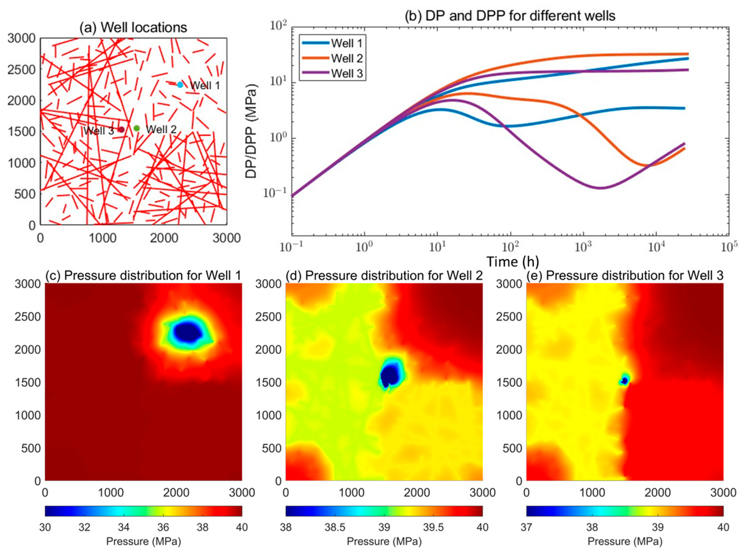
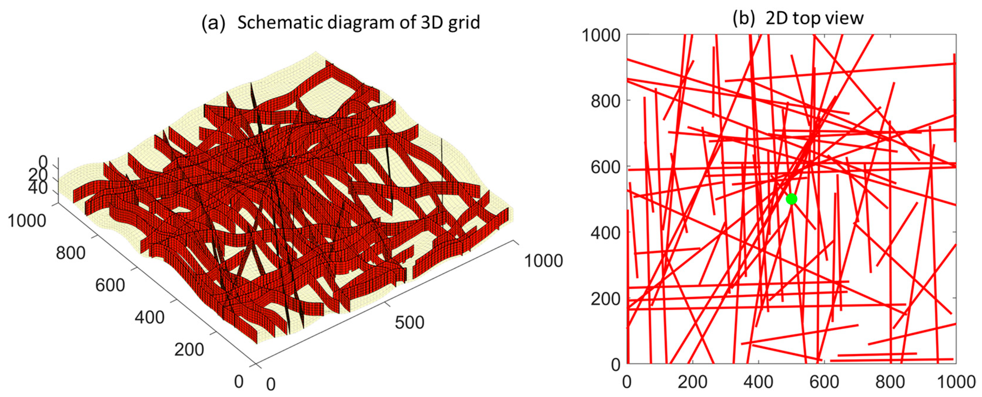
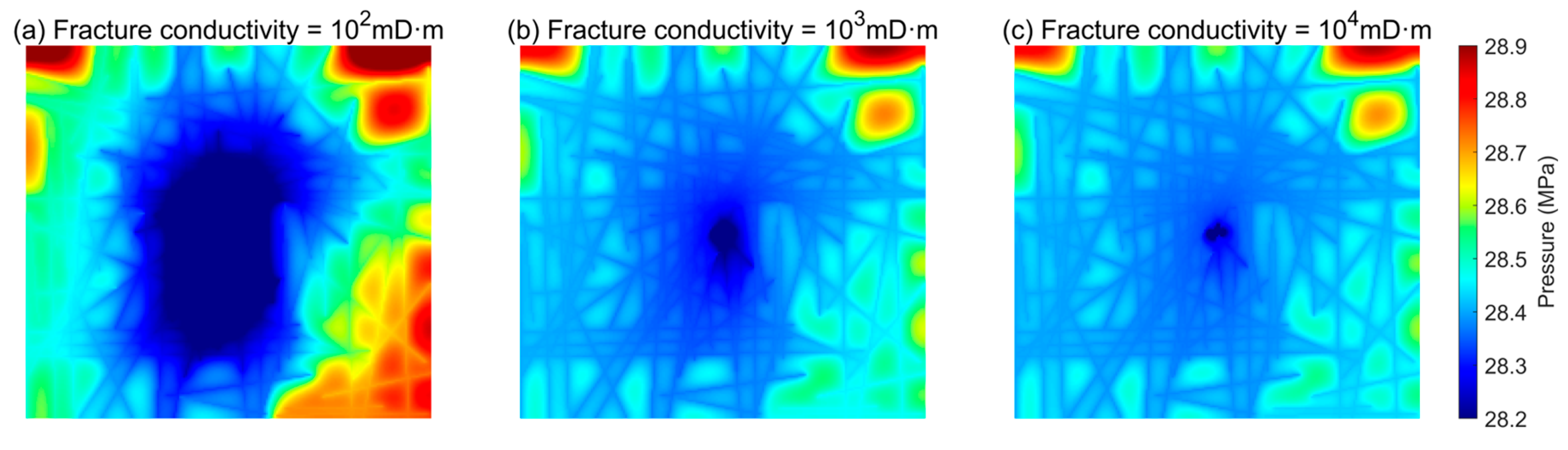
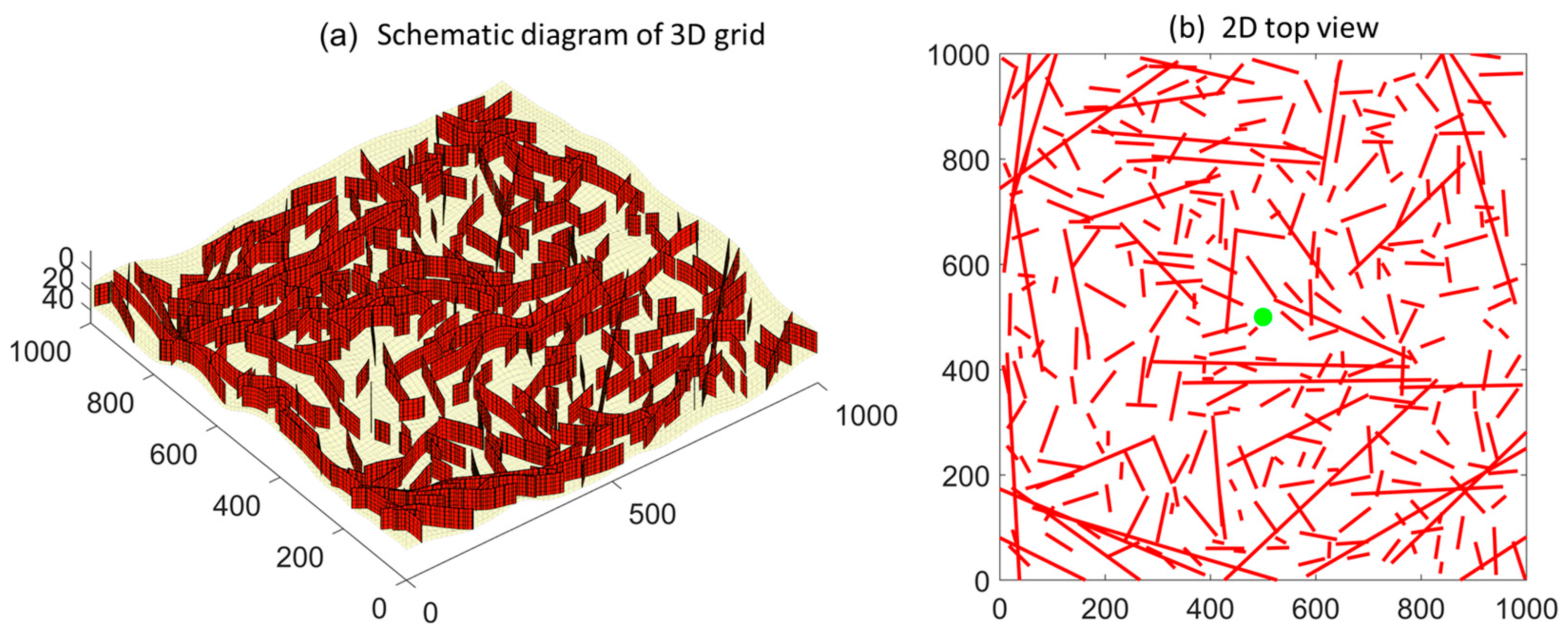
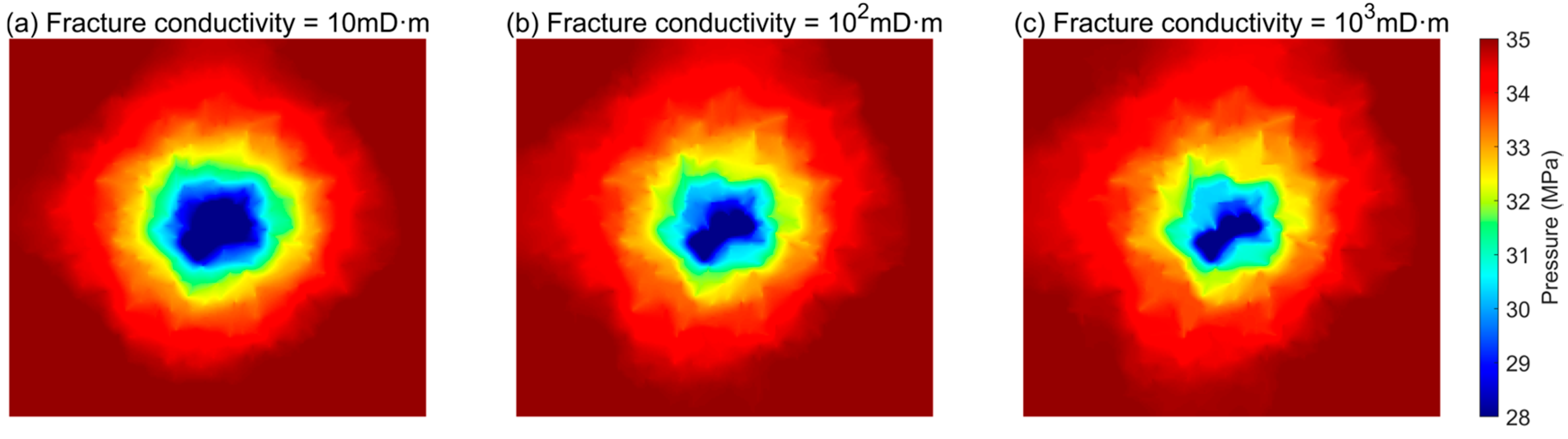
4.2. Effect of Natural Fractures on Pressure Transient Response

Figure 4 shows a schematic diagram of the model when large-scale fractures are developed in the reservoir. Figure 4a shows the 3D spatial fracture morphology, and Figure 4b shows the 2D plane fracture morphology, where the staggered distribution of red line segments represents the fracture morphology, and the green points represent vertical wells. The size of the gas reservoir geological model is 1000 m × 1000 m × 20 m, with the matrix grid dimensions being 201 × 201 × 5. A vertical well is located at the center of the gas reservoir, with a well radius of 0.1 m and a perforation thickness of 20 m. The original reservoir pressure is 40 MPa, the matrix porosity is 0.1, and the permeability is 0.01 × 10⁻³ μm². The fluid properties are consistent with those in Table 1. It is assumed that large-scale fractures are well developed in the reservoir, while small- to medium-scale fractures are less developed. The model includes 48 large-scale fractures, each with a length greater than 500 m, and 30 medium-scale fractures, with lengths ranging from 100 m to 500 m. The flow capacity of large-scale fractures is 1 × 10³ mD·m, while that of medium-scale fractures is 1 × 10² mD·m.

The DP test curves for the gas well were simulated for large-scale fracture flow capacities of 1 × 10⁴ mD·m, 1 × 10³ mD·m, and 1 × 10² mD·m. The pressure and PD log–log curves are shown in Figure 5. The research results indicate that the PD log–log curves exhibit three flow stages: the wellbore storage flow stage, the transient flow stage, and the complex large fracture flow stage. The pressure log–log curves show almost no difference, appearing as a horizontal straight line. In this geological model, the gas well’s PD curve, after passing through the wellbore storage and skin effect stages, directly enters the fracture flow stage. The greater the fracture conductivity (FC), the deeper the “cavity” in the PD curve, and the more pronounced the flow characteristic. Due to the high conductivity of the fractures, the pressure rapidly reaches the reservoir boundary. All DP curves eventually become straight lines with a slope of 1, influenced by the closed boundary.

Figure 6 shows the pressure contour map of the reservoir at t = 10,000 h under different fracture conductivities. The pressure profile clearly reflects the characteristics of natural gas flow along fractures in the large-scale developed formation. The pressure wave diffuses rapidly, quickly affecting the entire large-scale fracture zone, and the DP within the fractures is significantly greater than that in the matrix. Under the same production rate, the FC determines the DP rate of the large-scale fracture system. The smaller the FC, the greater the DP in the large-scale fracture system near the wellbore.

The geological model for the second type of medium-scale fractures is shown in Figure 7. In this model, large-scale fractures are underdeveloped, and the reservoir is primarily composed of medium- and small-scale fractures. The reservoir pressure, matrix properties, gas well, and fluid properties are consistent with those in the large-scale fracture model. The model includes 34 medium-scale fractures, each with a length of 100 m and an FC of 1000 mD·m. Additionally, there are 332 small-scale fractures, with an average length of 20 m and an FC of 100 mD·m.

The log–log pressure response curves for medium-scale fracture models with different fracture conductivities are shown in Figure 8. In this model, medium-scale and small-scale natural fractures are interconnected, leading to non-uniform pressure diffusion in multiple directions. Since there are no large-scale or medium-scale natural fractures directly connected to the wellbore, the pressure first experiences pseudo-radial flow in the near-wellbore region. When the pressure propagates to the medium-scale fracture system, the log–log curve exhibits characteristics of fracture flow. Changes in FC do not affect the flow stages outside the fracture flow phase. The larger the FC, the deeper the “concave” feature, and the more pronounced the fracture flow effect. This is because in a fracture system, FC directly reflects the equivalent permeability or conductivity of the fracture. The larger its value, the greater the fluid flow rate under the same pressure gradient. Combined with the Darcy formula in the seepage theory, it can be seen that the greater the fluid flow rate, the faster the pressure diffuses in the fracture. Mathematically, a larger FC increases the pressure attenuation term, resulting in faster pressure transmission, which in turn manifests as an earlier and deeper “depression” feature on the PD logarithmic curve. Additionally, due to the reduced fracture scale, the log–log pressure curve during the fracture flow phase differs significantly from that of large-scale fractures, with the log–log curve of the medium-scale fracture system gradually shifting upward.

The pressure profiles of medium-scale fracture models with different fracture conductivities at t = 10,000 h are shown in Figure 9. The research results indicate that medium-scale fractures dominate the pressure diffusion process, and the DP in regions with medium-scale fractures is greater than in regions with small-scale fractures. The larger the FC, the greater the pressure diffusion range, but the smaller the overall DP in the reservoir. Conversely, the smaller the FC, the slower the pressure diffusion along the fractures, and the greater the DP in the near-wellbore matrix region.

The third type of small-scale fracture geological model is shown in Figure 10. The reservoir pressure, matrix properties, gas well, and fluid properties are consistent with those of the first two geological models. In this model, small-scale fractures are heterogeneously developed in multiple directions, with a total of 674 small-scale fractures set in the entire model. The fracture lengths range from 10 to 50 m, and the FC is 1 × 10².

The log–log pressure response curves for different fracture conductivities in the small-scale fracture pattern are shown in Figure 11. Due to the small fracture length and conductivity, compared to the first and second types of fracture systems, the gas well exhibits a larger production DP, and the PD curve gradually shifts upward. When the FC is relatively high, the entire fracture system exhibits characteristics similar to a dual-porosity medium, and the log–log curve features show some similarity to those of the Warren–Root model. Since the small-scale natural fractures are relatively uniformly distributed, when the FC is low, the PD curve exhibits characteristics similar to system radial flow, appearing almost as a horizontal line. However, due to the influence of natural fractures, the DP in the fracture system is smaller than that in the matrix radial flow. Finally, under the influence of the outer boundary, all PD curves converge into a straight line with a slope of 1. For small-scale fracture systems, FC has a significant impact on the entire system. Changes in the FC lead to substantial variations in all stages of the log–log curve, except for in the wellbore storage and skin effect stages.

The pressure profile of the small-scale fracture system at t = 10,000 h is shown in Figure 12. The research results indicate that the pressure diffusion pattern in small-scale fractures exhibits a pseudo-radial flow pattern, spreading outward in all directions. The reason why pseudo-radial flow is formed in small-scale fracture networks is that small-scale fracture networks are usually composed of a large number of small and densely distributed fractures. Although individual fractures have obvious local heterogeneity, in the near-wellbore area, when the number of these fractures is sufficient and the distribution relatively uniform, the overall flow response will show similar behavior to that of a continuous homogeneous medium. Specifically, due to the limited conductivity of small-scale fractures, the fluid diffuses simultaneously along multiple paths in these fractures, and the local heterogeneous effects are averaged on a macroscopic scale, thus forming a pressure distribution feature similar to that of traditional radial flow. This phenomenon is called “pseudo-runoff flow”; that is, although there is actually a complex fracture network, the flow performance is similar to radial diffusion, which conforms to the basic characteristics of Darcy flow. The greater the FC, the faster the pressure diffuses, and the larger the final diffusion range. Conversely, the smaller the FC, the greater the DP amplitude in the matrix near the wellbore, and the more pronounced the radial pressure diffusion characteristics.

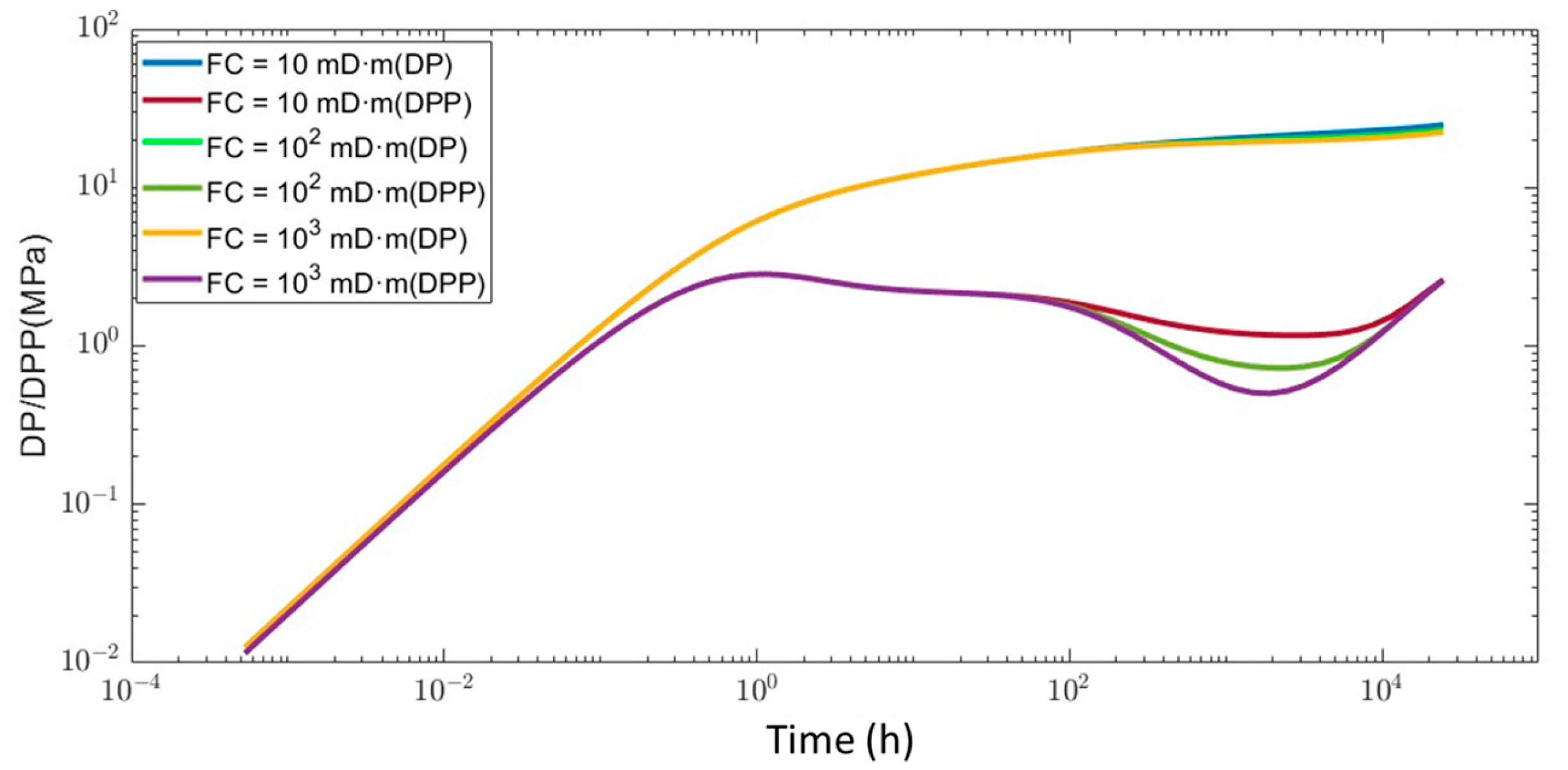
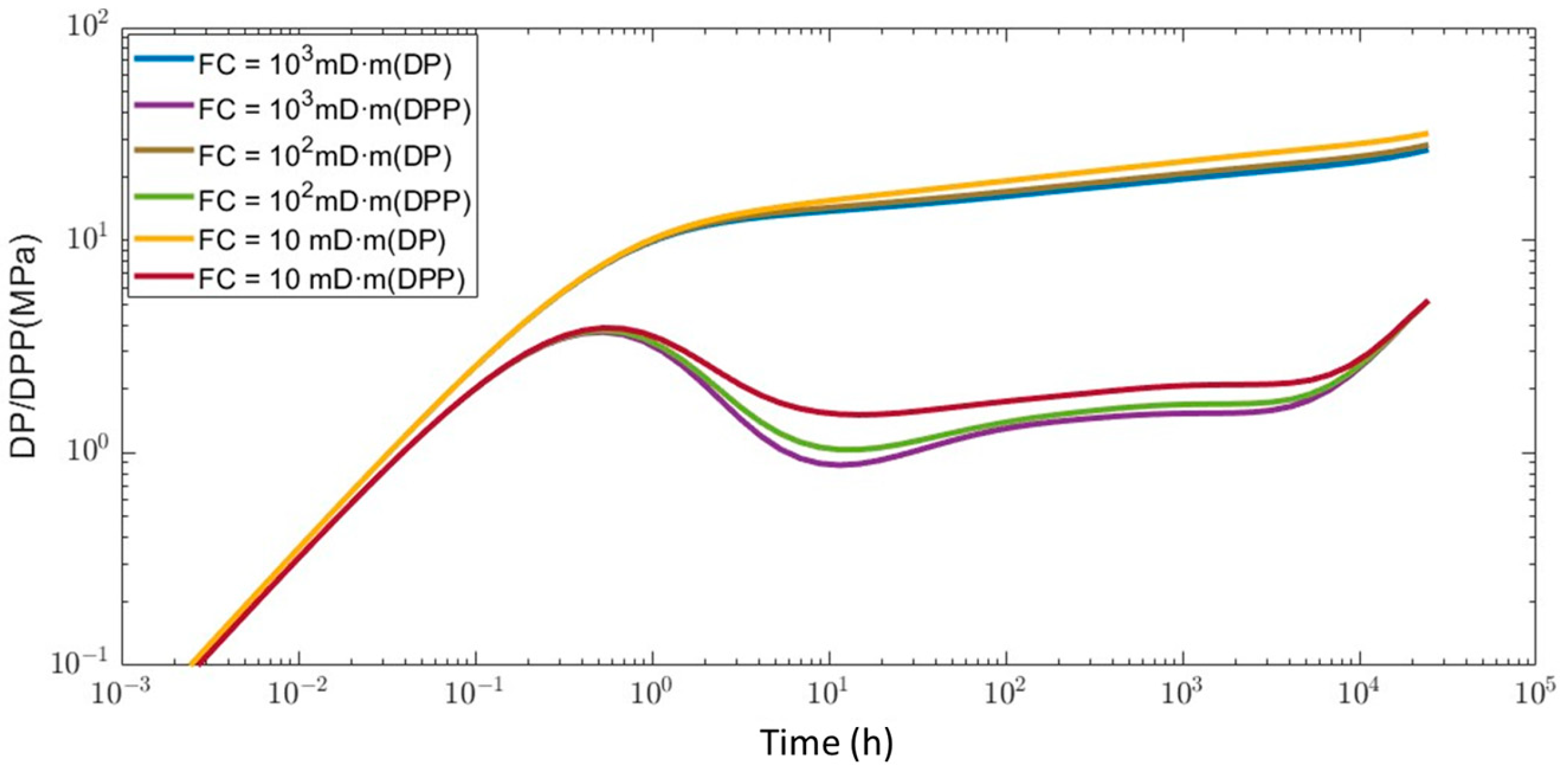
4.3. Influence of Nonlinear Flow Mechanisms on Pressure Transient

Figure 13 illustrates the impact of different λ values on the pressure response at a gas well production rate of 1 × 10⁴ m³/d. In the figure, the solid lines represent the DP, while the dashed lines represent the DPP. The curve before t = 1 h is the wellbore reservoir stage, and after t = 10 h, it enters the fracture flow stage, where the high-velocity non-Darcy flow has a small impact. When t = 100 h, the flow enters the matrix-dominated stage, and the influence of low-velocity non-Darcy flow begins to increase. The results indicate that the low-velocity non-Darcy effect has little influence on fracture-dominated flow but significantly affects matrix-dominated flow. In the late stage of the curve, low-velocity non-DF causes the pressure curve to shift upward, indicating that as the low-velocity non-Darcy effect intensifies, the reservoir experiences greater pressure depletion.

Figure 14 presents a comparison of the pressure responses between DF and high-velocity non-DF. The results show that non-DF generates additional DP, causing the pressure response curve to shift upward overall during the fracture-dominated flow stage. During the skin effect stage, the additional DP induced by high-velocity non-DF transforms into a rate-dependent pseudo-skin factor, leading to an upward shift in the high-velocity non-Darcy pressure response curve. In the early stage of the fracture-dominated flow stage, the additional DP caused by inertia results in increased pressure required to produce the same gas volume, thereby causing the pressure response curve to shift upward. In the late stage of the flow phase, fluid flow is primarily dominated by matrix flow, and the influence of high-velocity non-DF diminishes. The curve before t = 1 h is the wellbore reservoir stage, and after t = 10 h, it enters the fracture flow stage, where the high-velocity non-Darcy flow has a significant impact. After t = 5 × 10³ h, it enters the matrix-dominated flow stage, where the high-speed non-Darcy flow effect basically disappears on the pressure derivative but still has a significant impact on the overall pressure.

5. Field Application

Situated in the central Kelasu Structural Belt of Tarim Basin’s Kuqa Depression is the M Gas Field, where the primary hydrocarbon accumulation occurs in the Cretaceous Bashijiqike Formation. This sedimentary sequence represents a fan delta to braided river delta front depositional environment, exhibiting thick, laterally continuous sandstone units with limited interbed development. The reservoir demonstrates challenging matrix characteristics, showing porosity values between 2% and 8% (mean value: 6.13%) and permeability measurements ranging from 0.01 to 0.5 × 10⁻³ μm² (mean: 0.05 × 10⁻³ μm²). Subjected to significant tectonic compression and deformation forces, the reservoir exhibits extensive development of large-scale fracture networks. Characterized by burial depths ranging from 6000 to 8000 m, initial reservoir pressures of 90–136 MPa, and pressure coefficients between 1.6 and 1.85, this formation represents a distinctive ultra-deep, ultra-high-pressure fractured tight sandstone gas accumulation. The implementation of volume stimulation techniques prior to well production has become standard practice, with the Keshen Gas Field demonstrating particularly prominent multi-scale fracture characteristics.

The well KS1 is located at the structural top of the gas reservoir, with a daily gas production of 38.1 × 10⁴ m³ and no oil or water production. A pressure buildup test was conducted on the gas well in September 2021, lasting over 200 h. The well penetrated a reservoir thickness of 27.5 m, with a mid-formation pressure of 123.8 MPa and a temperature of 181.41 °C. The matrix porosity was 6.75%, and the gas specific gravity was 0.57. The pressure response curves from the DF model, the multi-scale flow model, and the actual bottomhole pressure are shown in Figure 15. The PD curve of the gas well does not exhibit a radial flow plateau. After the wellbore storage and skin effect stages, the curve immediately transitions into the fracture flow stage, showing a significant “concave” feature, indicating pronounced fracture flow characteristics. The overall curve behavior aligns with the pressure response characteristics of large-scale fracture development described earlier. The conventional dual-porosity well-test model cannot interpret the curve, and fitting is challenging. Consequently, a comprehensive numerical well-test analysis was performed utilizing the cornerpoint grid EDFM integrated with a multi-scale flow model, with comparative analysis conducted against the conventional DF model. The interpretation outcomes are detailed in

Table 2. Well-test double logarithmic curve interpretation results.

Parameter	Value	Unit
Wellbore storage factor	0.31	m3/MPa
Skin factor	0.18	dimensionless
Number of large-scale fractures	12	item
Average length of large-scale fractures	510	m
Large-scale FC	1.2 × 104	mD·m
Number of small- and medium-sized fractures	180	item
Average length of small- and medium-sized fractures	45	m
Conductivity of small- and medium-scale fractures	2.3 × 102	mD·m
Hydraulic fracture half length	74	m
Hydraulic FC	1.4 × 103	mD·m

, while the matching results are illustrated in Figure 15. The RMSE between the true DP value and the DP value fitted by the model in this paper is 0.0588, and the R² is 0.8778; the RMSE between the true DPP value and the fitted DPP value is 0.0167, and the R² is 0.7170. The RMSE between the Darcy model fitted DP value and the true DP value is 0.3932, the R² is −9.5276, the RMSE between the true DPP value and the Darcy fitted DPP value is 0.0193, and the R² is 0.6126, as shown in

Table 3. Table of fitting accuracy between Darcy model and this model.

	Darcy FlowF		Non-Darcy Flow
	R2	RMSE	R2	RMSE
DP	−5.0958	0.3932	0.8778	0.0588
DDP	0.6126	0.0193	0.717	0.0167

. Analysis reveals that the log–log pressure and PD curves generated by the DF model exhibit significant deviation from field measurements. In contrast, the log–log curves obtained through the multi-scale flow model developed in this research demonstrate excellent agreement with the observed data. These findings validate the reliability of the proposed model and establish a novel methodological approach for enhanced understanding of reservoir geological properties.

6. Conclusions

In this study, a numerical simulation model was established based on the embedded discrete fracture model (EDFM), considering the non-DF effects in both the matrix and fracture domains. It systematically evaluates the coupling mechanisms of multi-scale flow behaviors and natural fracture networks on the pressure transient response in fractured tight sandstone gas reservoirs. The main conclusions are as follows:

(1) The threshold pressure gradient in the matrix domain causes the PD curve to exhibit a significant “upward bending” feature in the late-time stage, while the high-velocity non-Darcy effect in fractures manifests as a “downward concave” phenomenon in the derivative curve. The coupling of these two non-DF mechanisms significantly alters the dynamic characteristics of pressure propagation. The traditional DF assumption underestimates the rate of reservoir pressure depletion;

(2) The spatial distribution patterns of natural fractures (density, orientation, and connectivity) play a significant role in regulating the pressure transient response. A high-density fracture network results in a “wide opening” shape in the PD curve, while as the fracture density decreases, the pressure response gradually transitions to a dual-porosity system behavior. The spatial configuration relationship between fracture orientation and the artificial fracture network significantly influences the anisotropic characteristics of pressure propagation;

(3) The numerical model developed in this study can effectively identify the contributions of multi-scale flow mechanisms to the pressure transient response in fractured tight gas reservoirs, providing a theoretical basis for well-test interpretation. The research results offer important insights for optimizing development strategies and hydraulic fracturing designs in tight gas reservoirs.

References

1. Jia, A.; Wei, Y.; Guo, Z.; Wang, G.; Meng, D.; Huang, S. Development status and prospect of tight sandstone gas in China. Nat. Gas Ind. B 2022, 9, 467–476. [Google Scholar] [CrossRef]
2. Wei, J.; Zhang, J.; Yong, Z. Characteristics of Tight Gas Reservoirs in the Xujiahe Formation in the Western Sichuan Depression: A Systematic Review. Energies 2024, 17, 587. [Google Scholar] [CrossRef]
3. Wu, Z.; Cui, C.; Wang, Z.; Sui, Y.; Jia, P.; Tang, W. Well Testing Model of Multiple Fractured Horizontal Well with Consideration of Stress-Sensitivity and Variable Conductivity in Tight Gas Reservoirs. Math. Probl. Eng. 2018, 2018, 1693184. [Google Scholar] [CrossRef]
4. Zhang, Y.; Zeng, L.; Lyu, W.; Sun, D.; Chen, S.; Guan, C.; Tang, L.; Shi, J.; Zhang, J. Natural fractures in tight gas sandstones: A case study of the Upper Triassic Xujiahe Formation in Xinchang gas field, Western Sichuan Basin, China. Geol. Mag. 2021, 158, 1543–1560. [Google Scholar] [CrossRef]
5. Mohammed, I.; Olayiwola, T.O.; Alkathim, M.; Awotunde, A.A.; Alafnan, S.F. A review of pressure transient analysis in reservoirs with natural fractures, vugs and/or caves. Pet. Sci. 2021, 18, 154–172. [Google Scholar] [CrossRef]
6. Berre, I.; Doster, F.; Keilegavlen, E. Flow in Fractured Porous Media: A Review of Conceptual Models and Discretization Approaches. Transp. Porous Media 2019, 130, 215–236. [Google Scholar] [CrossRef]
7. Kharrat, R.; Ott, H. A Comprehensive Review of Fracture Characterization and Its Impact on Oil Production in Naturally Fractured Reservoirs. Energies 2023, 16, 3437. [Google Scholar] [CrossRef]
8. Tarhuni, M.-N.; Sulaiman, W.-R.; Jaafar, M.-Z.; Milad, M.; Alghol, A.-M. A Review of the Dynamic Modeling Approaches for Characterizing Fluid Flow in Naturally Fractured Reservoirs. Energy Eng. 2021, 118, 761–795. [Google Scholar] [CrossRef]
9. Jiang, T.; Sun, H.; Xiao, X.; Zhu, S.; Ouyang, W.; Tang, Y. Multi-scale flow mechanism and water control strategy of ultra-deep multi-porosity fractured tight sandstone gas reservoirs. Front. Energy Res. 2022, 10, 977439. [Google Scholar] [CrossRef]
10. Sun, H.; Ouyang, W.; Zhu, S.; Wan, Y.; Tang, Y.; Cao, W. A new numerical well test method of multi-scale discrete fractured tight sandstone gas reservoirs and its application in the Kelasu Gas Field of the Tarim Basin. Nat. Gas Ind. B 2023, 10, 103–113. [Google Scholar] [CrossRef]
11. Hui, G.; Chen, Z.; Schultz, R.; Chen, S.; Song, Z.; Zhang, Z.; Song, Y.; Wang, H.; Wang, M.; Gu, F. Intricate Unconventional Fracture Networks Provide Fluid Diffusion Pathways to Reactivate Pre-Existing Faults in Unconventional Reservoirs. Energy 2023, 282, 128803. [Google Scholar] [CrossRef]
12. Geng, S.; Li, C.; Zhai, S.; Gong, Y.; Jing, M. Modeling the Mechanism of Water Flux in Fractured Gas Reservoirs with Edge Water Aquifers Using an Embedded Discrete Fracture Model. J. Energy Resour. Technol. 2022, 145, 033002. [Google Scholar] [CrossRef]
13. Yao, J.; Ding, Y.; Sun, H.; Fan, D.; Wang, M.; Jia, C. Productivity Analysis of Fractured Horizontal Wells in Tight Gas Reservoirs Using a Gas–Water Two-Phase Flow Model with Consideration of a Threshold Pressure Gradient. Energy Fuels 2023, 37, 8190–8198. [Google Scholar] [CrossRef]
14. Nie, R.-S.; Fan, X.; Li, M.; Chen, Z.; Deng, Q.; Lu, C.; Zhou, Z.-L.; Jiang, D.-W.; Zhan, J. Modeling transient flow behavior with the high velocity non-Darcy effect in composite naturally fractured-homogeneous gas reservoirs. J. Nat. Gas Sci. Eng. 2021, 96, 104269. [Google Scholar] [CrossRef]
15. Zhu, W.; Liu, Y.; Shi, Y.; Zou, G.; Zhang, Q.; Kong, D. Effect of dynamic threshold pressure gradient on production performance in water-bearing tight gas reservoir. Adv. Geo-Energy Res. 2022, 6, 286–295. [Google Scholar] [CrossRef]
16. Fu, J.; Su, Y.; Li, L.; Wang, W.; Wang, C.; Li, D. Productivity model with mechanisms of multiple seepage in tight gas reservoir. J. Pet. Sci. Eng. 2022, 209, 109825. [Google Scholar] [CrossRef]
17. Geng, S.; Li, C.; Li, Y.; Zhai, S.; Xu, T.; Gong, Y.; Jing, M. Pressure transient analysis for multi-stage fractured horizontal wells considering threshold pressure gradient and stress sensitivity in tight sandstone gas reservoirs. Gas Sci. Eng. 2023, 116, 205030. [Google Scholar] [CrossRef]
18. Zhao, L.; Jiang, H.; Wang, H.; Yang, H.; Sun, F.; Li, J. Representation of a new physics-based non-Darcy equation for low-velocity flow in tight reservoirs. J. Pet. Sci. Eng. 2020, 184, 106518. [Google Scholar] [CrossRef]
19. Yin, P.; Zhao, C.; Ma, J.; Huang, L. A Unified Equation to Predict the Permeability of Rough Fractures via Lattice Boltzmann Simulation. Water 2019, 11, 1081. [Google Scholar] [CrossRef]
20. Geng, S.; Wang, Q.; Zhu, R.; Li, C. Experimental and numerical investigation of Non-Darcy flow in propped hydraulic fractures: Identification and characterization. Gas Sci. Eng. 2024, 121, 205171. [Google Scholar] [CrossRef]
21. Geng, S.; He, X.; Zhu, R.; Li, C. A new permeability model for smooth fractures filled with spherical proppants. J. Hydrol. 2023, 626, 130220. [Google Scholar] [CrossRef]
22. Liu, X.; Geng, S.; Sun, J.; Li, Y.; Guo, Q.; Zhan, Q. Novel coupled hydromechanical model considering multiple flow mechanisms for simulating underground hydrogen storage in depleted low-permeability gas reservoir. Int. J. Hydrog. Energy 2024, 85, 526–538. [Google Scholar] [CrossRef]
23. Najafian Jazi, F.; Ghasemi-Fare, O.; Rockaway, T.D. Natural convection effect on heat transfer in saturated soils under the influence of confined and unconfined subsurface flow. Appl. Therm. Eng. 2024, 237, 121805. [Google Scholar] [CrossRef]
24. Lie, K.-A. An Introduction to Reservoir Simulation Using MATLAB/GNU Octave: User Guide for the MATLAB Reservoir Simulation Toolbox (MRST); Cambridge University Press: Cambridge, UK, 2019. [Google Scholar] [CrossRef]
25. Liu, X.; Geng, S.; Hu, P.; Li, Y.; Zhu, R.; Liu, S.; Ma, Q.; Li, C. Blasingame production decline curve analysis for fractured tight sand gas wells based on embedded discrete fracture model. Gas Sci. Eng. 2024, 121, 205195. [Google Scholar] [CrossRef]
26. Luo, H.; Deng, H.; Xiao, H.; Geng, S.; Hou, F.; Luo, G.; Li, Y. A Transient-Pressure-Based Numerical Approach for Interlayer Identification in Sand Reservoirs. Fluid Dyn. Mater. Process. 2024, 20, 641–659. [Google Scholar] [CrossRef]
Figure 1. Verification grid of single-phase flow model.
Processes 13 01163 g001
Figure 2. Comparison of the well-test pressure profile and corresponding PD curve of the EDFM numerical model developed in this paper and Saphir commercial software under single-phase flow conditions.
Processes 13 01163 g002
Figure 3. Comparison of well-test curves and pressure profiles at different fracture scales and development degrees.
Processes 13 01163 g003
Figure 4. Type 1 geological model (large-scale fracture development).
Processes 13 01163 g004
Figure 5. Transient response curve of bottomhole pressure in the first geological model with different FCs.
Processes 13 01163 g005
Figure 6. Pressure profile of large-scale fracture model with different FC.
Processes 13 01163 g006
Figure 7. The second type of geological model (development of small- and medium-scale fractures).
Processes 13 01163 g007
Figure 8. Transient response curve of bottomhole pressure under different FC of the second geological model.
Processes 13 01163 g008
Figure 9. Pressure profiles of small- and medium-scale fracture models with different FC.
Processes 13 01163 g009
Figure 10. The third type of geological model (small-scale fractures are developed; medium- and large-scale fractures are not developed).
Processes 13 01163 g010
Figure 11. Transient response curve of bottomhole pressure under different FC of the third geological model.
Processes 13 01163 g011
Figure 12. Pressure profile of small-scale fracture model with different FC.
Processes 13 01163 g012
Figure 13. Effect of low-velocity non-DF on bottomhole pressure response.
Processes 13 01163 g013
Figure 14. Comparison of pressure response curves under DF and high-velocity non-DF.
Processes 13 01163 g014
Figure 15. Fitting diagram of bottomhole pressure response curve of KS1 well.
Processes 13 01163 g015