Abstract
Extreme scenarios involving abnormal load fluctuations pose serious challenges to the safe and stable operation of power systems. To address these challenges, an ultra-short-term load forecasting model is proposed, specifically designed for extreme conditions. The model combines density-based spatial clustering of applications with noise (DBSCAN), random search Bayesian optimization (RSBO), bidirectional gated recurrent units (BiGRUs), k-nearest neighbor (KNN), and an attention mechanism, enhanced by a fine-tuning strategy to improve forecasting accuracy. Firstly, the original load data are reconstructed weekly, and extreme scenarios are identified using the DBSCAN. Secondly, the RSBO is employed to optimize model parameters within the high-dimensional search space. To further refine performance, the final fully connected layer is fine-tuned to adapt to extreme conditions. Finally, case studies demonstrate that the proposed approach reduces the root mean square error (RMSE) by 12.37% and the mean absolute error (MAE) by 6.73% compared to benchmark models, achieving superior accuracy under all tested extreme scenarios.
1. Introduction
In recent years, extreme scenarios in power systems have become more frequent, driven by factors such as climate change and the ongoing energy transition [1,2]. These scenarios pose serious risks to the safe and stable operation of power systems. As a result, accurately identifying extreme events and improving load forecasting under such conditions remain critical challenges for both researchers and practitioners [3,4,5].
Currently, the methods for extreme scenario extraction generally fall into two categories: clustering-based approaches and heuristic techniques. Clustering methods group similar data points to reveal underlying patterns in load behavior. For example, in [6], self-organizing maps were used to cluster net load time series and extract periods with the highest and lowest load values as extreme scenarios. In [7], a clustering algorithm was employed to extract extreme scenarios, and the extracted scenarios were characterized by high load and large peak-to-valley differences. Similarly, in [8], the minimum cumulative distance method was used to cluster load data. Scenarios were considered extreme if their distance from the cluster center exceeded the upper quartile plus 1.5 times the interquartile range. Heuristic methods, on the other hand, identify patterns and extreme conditions by summarizing existing data and expert knowledge. For example, in [9], considering weather and photovoltaic effects, by using similar day selection, scenes with significant load fluctuations or large peak-to-valley differences were extracted as extreme scenarios. Further analysis from the perspective of data changes classifies extreme scenarios as those with significantly different load fluctuations compared to normal scenarios, characterized by low occurrence probability and high randomness. The aforementioned studies extract extreme scenarios from multiple perspectives; however, these methods still have limitations in capturing abnormal fluctuations, covering extreme situations, and handling unlabeled data.
On the other hand, current forecasting models mainly fall into two categories: ensemble learning models and neural network models. Machine learning models include LightGBM, XGBoost, and CatBoost. For example, in [10], a LightGBM-based forecasting model was proposed, which could enhance model performance through error correction mining and feature derivation. Similarly, in [11], an XGBoost-based two-layer cooperative real-time correction ultra-short-term photovoltaic forecasting model was proposed, which linked baseline forecasting with a real-time correction to avoid a drop in forecasting accuracy during transitional weather conditions. To address the low forecasting accuracy of machine learning models when dealing with large-scale and sparse-feature datasets, neural networks were introduced. Neural networks, with their powerful nonlinear fitting capabilities and ability to handle high-dimensional data, can be utilized to significantly improve load forecasting accuracy. Neural network models normally include convolutional neural networks (CNNs), long short-term memory (LSTM), gated recurrent units (GRUs), and Transformers, among others. For example, in [12], the forecasting accuracy was improved by leveraging the advantages of CNN feature extraction and LSTM forecasting. Similarly, in [13], a load forecasting method with higher accuracy was developed based on a temporal fusion transformer. Compared with GRUs and LSTM [14], bidirectional gated recurrent units (BiGRUs) could capture both forward and backward information in the input sequence [15], thereby providing a better understanding of contextual relationships.
To dynamically focus on the key parts of the input data and enhance the model performance and generalization capabilities, the attention mechanism—a crucial component of deep learning—has been widely applied in load forecasting. However, as the data scale and sequence length increase, the computational complexity of traditional attention mechanisms rises sharply, which has become a major bottleneck. To address this challenge, k-nearest neighbor attention (KNN-Attention) was introduced in [16], which reduced computational complexity by considering only the k most relevant keys for each query and also mitigated the impact of noise. Inspired by this, in the paper, the KNN-Attention model will be integrated into the forecasting framework, with the aim of improving forecasting accuracy in some extreme scenarios.
In addition, transfer learning could improve the model’s performance on the target task by transferring the knowledge learned from one task to another related task [17]. For example, in [18], a forecasting model based on feature selection and multi-level deep transfer learning was proposed, which could effectively address the problem of insufficient training data. Similarly, in [19], a method combining CNNs and LSTM for pre-training was proposed, and information from neighboring wind farms was extracted through transfer learning to improve forecasting accuracy. Through transfer learning methods and personalized training strategies, forecasting accuracy could be enhanced. However, existing fine-tuning strategies require high-quality source domain data, and when the quality of the source domain data is poor, it is difficult to guarantee the forecasting accuracy.
Most existing research in load forecasting focuses on normal operating conditions, while relatively few studies address the challenges of forecasting in extreme scenarios. Moreover, current optimization methods used in load forecasting models often struggle with complex, high-dimensional parameter spaces and can be limited in their ability to improve accuracy under extreme conditions [20,21]. Based on the above discussions, an ultra-short-term load forecasting approach is designed for extreme scenarios. Weekly data restructuring is combined with DBSCAN to assess data density, where low-density regions are identified as extreme scenarios. A BiGRU-KNN-Attention model is then used to perform forecasting, offering a balance between computational efficiency and the ability to capture key temporal features. To further improve performance, a random search Bayesian optimization (RSBO) strategy is applied for efficient parameter tuning. Finally, a fine-tuning strategy based on transfer learning is introduced to enhance model adaptability and generalization in unseen extreme scenarios. The main contributions of this paper are as follows:
- (1)
- A novel use of DBSCAN for identifying extreme load scenarios is presented, addressing the challenge of insufficient validation data in rare and critical events.
- (2)
- An integrated forecasting framework is introduced, which captures key features and long-term dependencies in the data. The use of RSBO enhances model accuracy and robustness, particularly under extreme conditions.
- (3)
- A fine-tuning approach based on transfer learning is developed to improve the model’s adaptability and generalization performance in extreme scenarios.
The rest of the paper is organized as follows: Section 2 presents the methodology in detail, covering data reconstruction, scenario extraction, model design, optimization, fine-tuning, and evaluation metrics. Section 3 provides an analysis and discussion of the forecasting results across different models and datasets under extreme scenarios. Section 4 concludes the study and outlines future research directions.
2. Methodology
2.1. Data Reconstruction
To evaluate the forecasting accuracy of the proposed model under various extreme conditions, extreme scenarios were extracted directly from the data. Given the need to identify and analyze medium-to-long-term extreme scenarios, the raw electricity load data must first be appropriately reconstructed. Electricity load data are typically recorded in time series format. As highlighted in [22], organizing these data on a weekly basis helps capture both short-term fluctuations and long-term trends, thus enhancing the efficiency and completeness of the analysis. In [23], it was noted that the key issue in scenario clustering lies not in the classification function (linear or nonlinear), but in selecting features that can be effectively distinguished. Expanding on this, ref. [24] introduced a clustering approach based on interpretable and distinctive features, which involved a two-step process that focused on key statistical measures such as the maximum and minimum load values for each period. In this study, DBSCAN was applied to reconstruct the data on a weekly basis. For each week, the average, maximum, minimum, standard deviation, peak-to-valley difference, skewness, and kurtosis of the electricity load values were calculated. These statistics effectively captured the load variations over the week and served as critical features for the subsequent clustering analysis. This reconstructed weekly dataset formed a solid foundation for identifying extreme scenarios on a medium-to-long-term scale.
2.2. Extreme Scenario Extraction
In the context of this paper, an extreme scenario refers to a situation where load variations significantly differ from typical patterns, often due to factors such as climate changes or equipment failures. In [25], extreme scenarios were identified using clustering algorithms. By extracting scenarios that deviate significantly from the clustering center, sparse regions are selected as extreme scenarios. DBSCAN, a density-based clustering method, offers several advantages over traditional clustering techniques. Unlike other methods, DBSCAN does not require the number of clusters to be predefined. Instead, it adaptively identifies core points based on density differences, allowing it to detect complex and irregular clusters. Moreover, the DBSCAN is particularly effective in identifying extreme scenarios due to its robust handling of noise. It marks isolated points in low-density regions as outliers, rather than forcing them into existing clusters, making it well suited for analyzing rare and exceptional events in load forecasting.
The distance between two samples can be defined as
where is the number of datasets.
The -neighborhood of a sample consists of all samples within a specified distance , which can be expressed as
where is the entire dataset.
A sample is classified as a core sample if the number of samples within its -neighborhood is at least the predefined threshold , which can be expressed as
Each core sample forms the center of a cluster. All points in its -neighborhood are included in the cluster, and this process continues recursively, expanding neighborhoods until no more core samples can be added. The collection of all extreme samples can be expressed as
where is a cluster. is the number of clusters.
Finally, extreme samples identified through clustering are mapped back to their corresponding time series or observation intervals in the original dataset. This reverse-mapping process generates the extreme scenario dataset.
2.3. Load Forecasting Model
2.3.1. BiGRU-KNN-Attention
In load forecasting, data typically exhibit significant time dependence. By addressing the long-term dependency problem, the model can capture the dynamic patterns of load variation over time, thus improving forecasting performance for extreme scenarios. LSTM and its variant GRU effectively solve the gradient vanishing problem in RNNs. GRU, having fewer parameters than LSTM, is computationally more efficient and easier to implement, with faster convergence. The main parameters of the GRU network are calculated as
where represents the value of the reset gate. denotes the Sigmoid activation function, and represent the weight matrices of the reset gate, applied to the current input and the previous hidden state , respectively. represents the candidate hidden state at the current time step, is the hyperbolic tangent activation function. denotes the Hadamard product, and are the weight matrices for the candidate hidden state. The hidden state at the current time step is denoted by , and represents the value of the update gate.
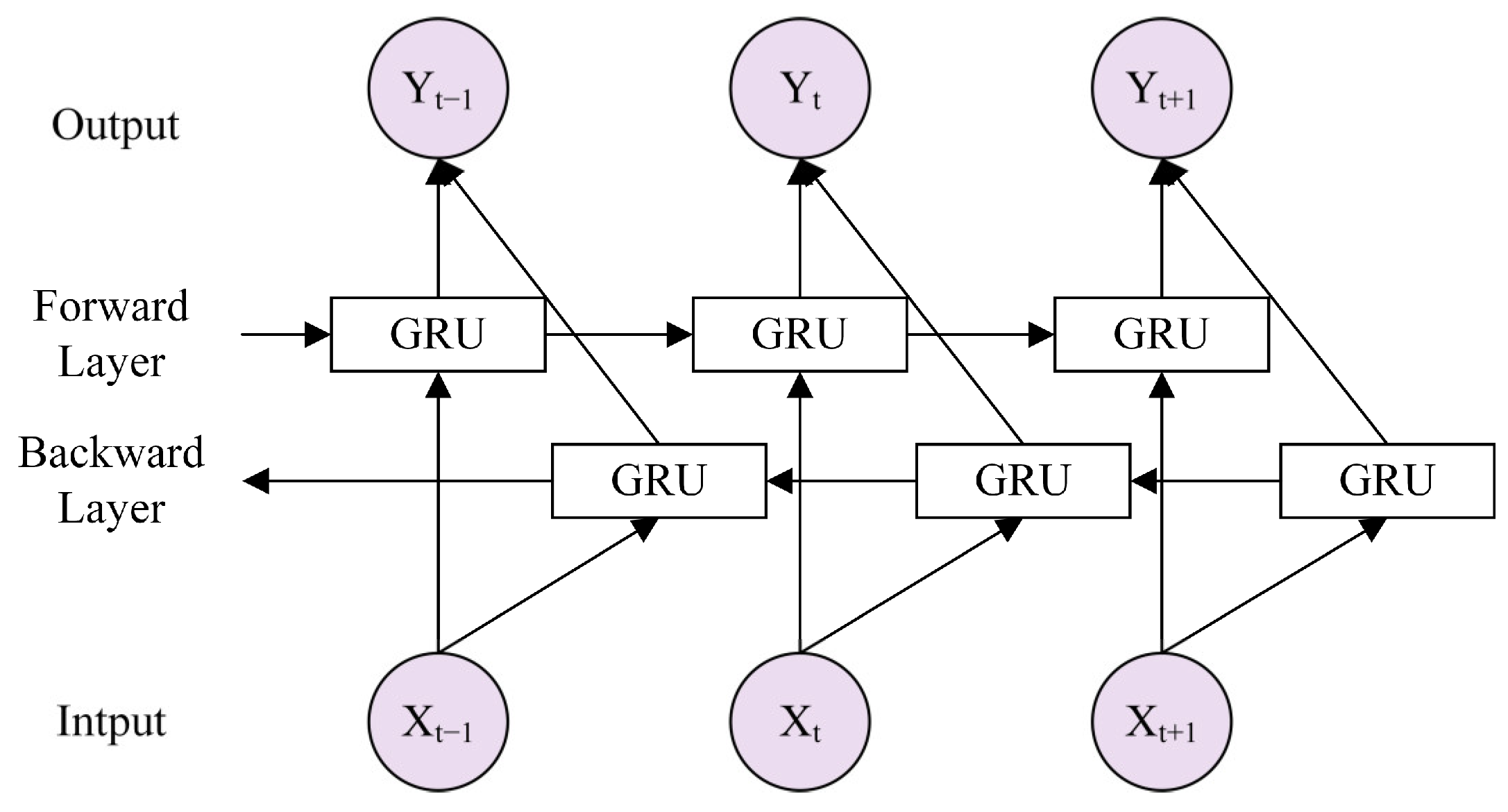
Compared with GRU, the BiGRU can process the forward and backward information of the input sequence simultaneously, capturing the context information more comprehensively. BiGRU consists of two stacked GRUs, and the output is determined by the states of the two GRUs. Assuming the first layer is forward and the second layer is backward, the hidden states of each layer are defined as and . Then, the final hidden state can be calculated as
where and are the hidden states of the forward GRU layer at the previous time step and the backward GRU layer at the next time step, respectively. and are the weight matrices for the forward and backward hidden states, and represents the bias term. The structure is shown in Figure 1.
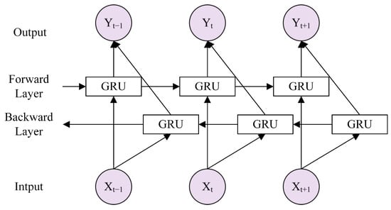
Figure 1.
Structure of BiGRU.
After calculating the dot product of the query and key, KNN-Attention selects only the top elements from each row for computation, effectively filtering out irrelevant tokens. Compared to the standard attention mechanism, KNN-Attention improves prediction accuracy by focusing on high-weight dot products to identify key long-term dependencies. Moreover, its low-scale selection process effectively reduces noise, which is a common issue in standard attention mechanisms. Especially in extreme cases where the input feature distribution may be anomalous, KNN-Attention maintains model stability by focusing on critical points, mitigating the impact of distribution bias on prediction, and reducing forecasting errors. This approach not only retains the advantages of self-attention mechanisms, but also demonstrates significant improvements in enhancing locality and overall model performance. The specific calculation formulas are as follows.
First, compute the scaled dot product of the query matrix and key matrix, which can be expressed as
where is the attention matrix, is the matrix dimension, and and are the query and key, respectively.
Then, the elements can be selected from each row as follows:
At the same time, the softmax function is applied to the attention matrix after selecting the elements
Finally, the new value matrix can be calculated by multiplying the KNN attention weights with the values, which is given by
The main process of the BiGRU-KNN-Attention model built on this is as follows: First, the input data are passed to the BiGRU layer, and its bidirectional structure is used to extract time series features from the forward and reverse directions. The output of the BiGRU is passed to the attention mechanism layer, which selects the top k most relevant data points in each time step by calculating the similarity score between the query and the key, and assigns higher weights to these key data points. Therefore, the attention mechanism can focus on the most representative information fragments in the time series, further enhancing the focus on important features and patterns. Secondly, the output is flattened into a one-dimensional vector and passed to the fully connected layer to integrate features. Finally, the model combines the bidirectional feature extraction capability with the information-focusing capability to further improve the load forecasting accuracy in extreme scenarios.
2.3.2. RSBO
The RSBO module was utilized to improve the forecasting ability of the BiGRU-KNN-Attention model. First, the random search method is used to explore a wide hyperparameter space, randomly selecting different hyperparameter combinations and training the model to find the optimal initial hyperparameter range. Then, based on the results of the random search, Bayesian optimization is applied to fine-tune the hyperparameters, further accelerating the model’s convergence. Finally, the combination of broad exploration in the initial stage and fine-tuned optimization results in better hyperparameter selection. The process of RSBO can be represented as follows.
The model randomly selects hyperparameter combinations within a given range for training. For each set of hyperparameters, the model’s loss function can be expressed as
where is the number of samples. is the true value. is the forecasted value, and represents the model parameter.
Bayesian optimization is employed to fine-tune the hyperparameters by constructing a Gaussian process regression model. This approach iteratively evaluates the objective function, which can be expressed as
where represents the objective function. is the hyperparameter, is the evaluation value of the objective function, and is the noise term.
In each optimization iteration, Bayesian optimization calculates the expected improvement as
where is the current optimal hyperparameter. Bayesian optimization can accelerate the search and further improve the model’s performance.
2.3.3. Fine-Tuning
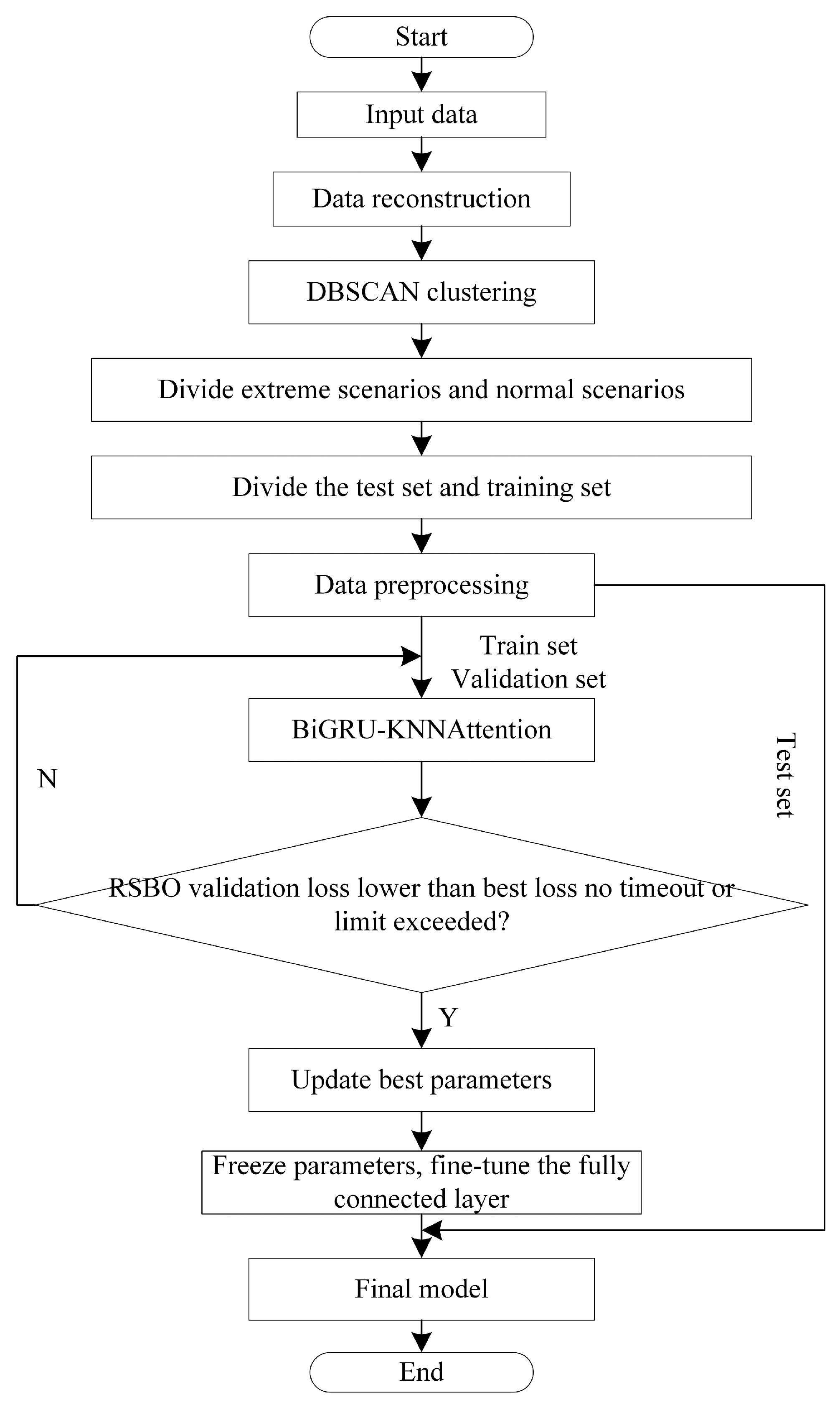
After the initial model training and optimization, a fine-tuning strategy as applied to further enhance performance. Most of the parameters in the pre-trained model were kept fixed, while only the last fully connected layer was updated. This approach preserves the model’s ability to extract general features while minimizing the risk of forgetting previously learned patterns. The fine-tuning strategy retrains the model using the training dataset, improving the model’s adaptability to the task and fully extracting information from the data. During fine-tuning, a smaller learning rate is used to ensure that the updates to the parameters of the fully connected layer are relatively small, avoiding drastic parameter changes that could degrade the model’s performance. Additionally, by monitoring the loss changes on the validation set, the training process is dynamically evaluated, and the optimization direction of the fully connected layer is adjusted. The flowchart is shown in Figure 2.
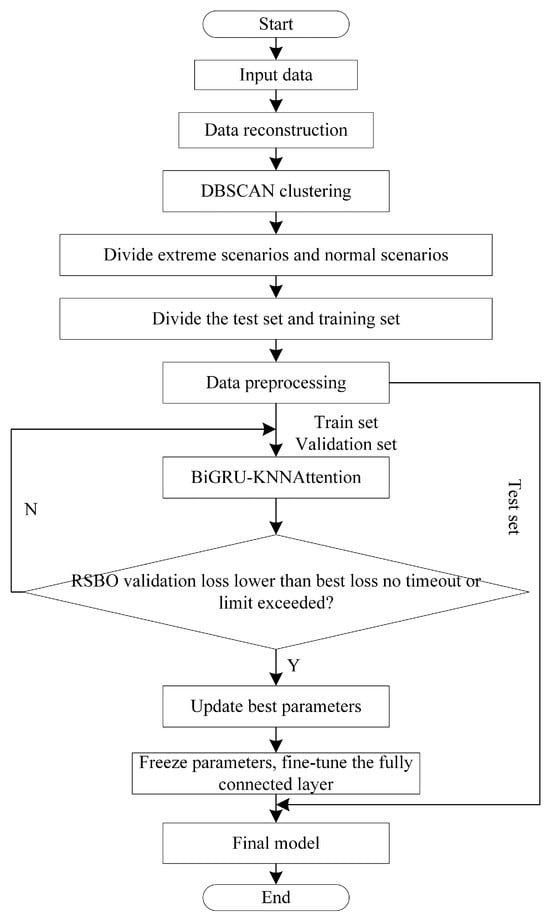
Figure 2.
Flow chart of load forecasting in extreme scenarios.
2.4. Data Acquisition and Models’ Parameters
Accurate load forecasting plays a critical role in power grid planning, operation, and scheduling. To validate the proposed method, this study uses load data from the Irish region, sourced from the Global Energy Forecasting Competition 2014 (GEFCom2014). The dataset contains 78,888 hourly records of load and temperature data spanning from 1 January 2006 to 31 December 2014.
The data have a resolution of 1 h. In this study, temperature was used as the input feature, while load was the target variable. Three periods characterized by extreme load conditions, 5–11 January, 6–12 April, and 29 June–5 July 2014, were selected as test sets to evaluate forecasting performance under challenging scenarios. The dataset exhibits clear periodic patterns, which the model must learn to capture. To help the model recognize temporal dependencies and historical trends, a time-lag of 24 h was applied based on insights from preliminary tests. This lag strikes a balance between forecasting accuracy and computational efficiency. To evaluate generalization ability and ensure reliable forecasting in unseen scenarios, each extreme period was divided into training and validation sets using a 9:1 ratio before model inference. The forecasting results are assessed using the evaluation metrics described in Section 3.2, offering a comprehensive view of the model’s stability and applicability.
All simulations are implemented in Python 3.9 using the PyTorch framework, and training is accelerated with an NVIDIA GeForce RTX 4060 GPU. The key parameters of each model component are detailed in Table 1.

Table 1.
The main parameters of the model.
2.5. Evaluation Metrics
The accuracy of the load forecasting model is evaluated using three metrics: root mean squared error (RMSE), mean absolute error (MAE), and accuracy. These indicators are formulated as
where represents the number of samples, is the average of the true values, is the actual value, and is the forecasted value.
2.6. The Load Forecasting Framework for Extreme Scenarios
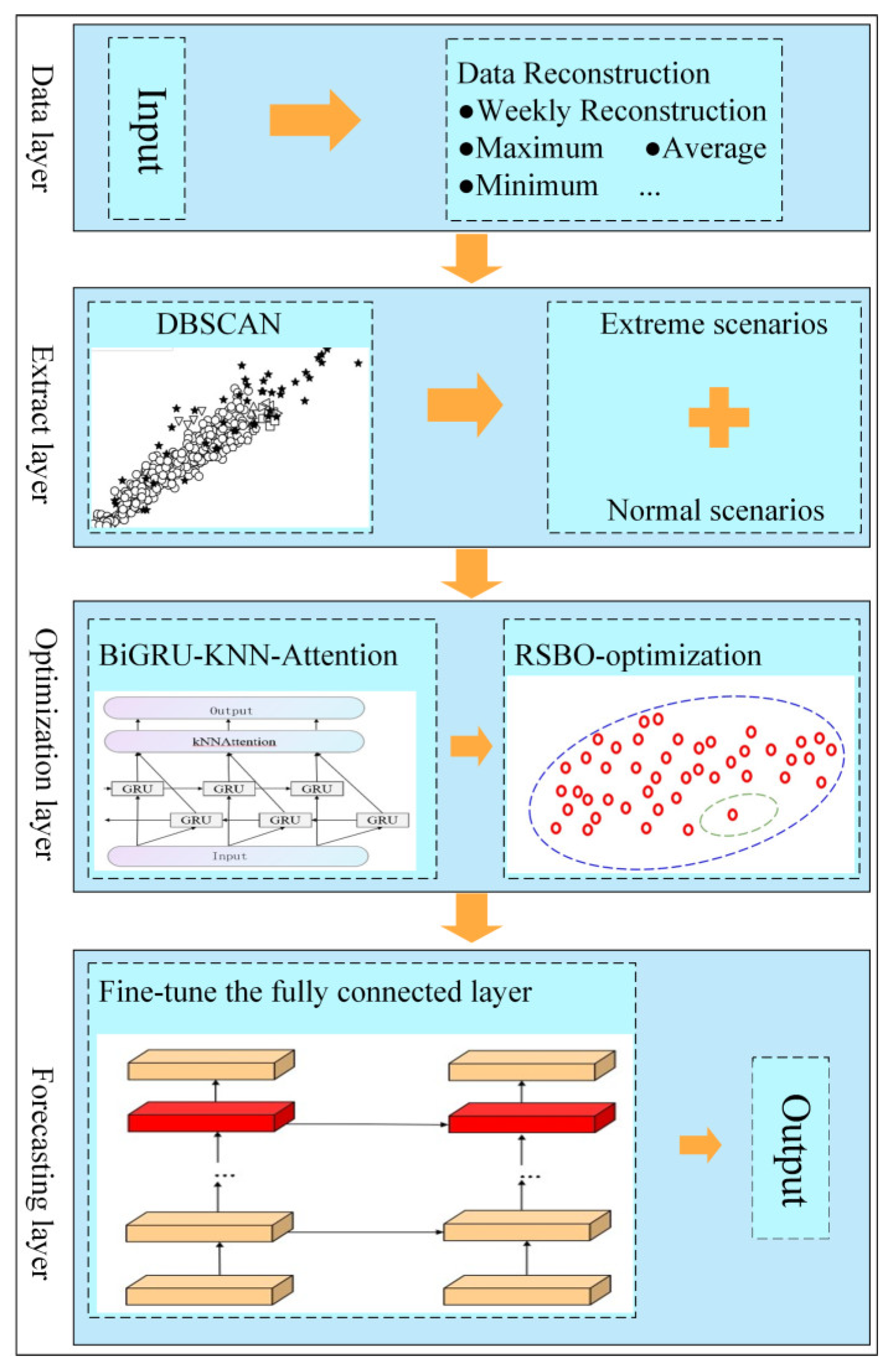
The proposed method for improving load forecasting accuracy in extreme scenarios consists of five key modules: data reconstruction, extreme scenario extraction, load forecasting, model optimization, and forecasting evaluation. The overall architecture is illustrated in Figure 3. The process is as follows:
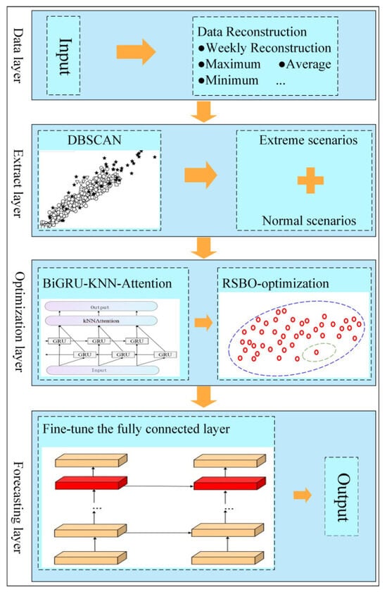
Figure 3.
Architecture of the proposed forecasting model.
- (1)
- The data are reconstructed on a weekly basis, with key features extracted. DBSCAN is then used to identify extreme scenarios from the dataset.
- (2)
- The time series data are processed through the BiGRU layer, which captures temporal dependencies. The features extracted by BiGRU are then sent to the KNN-Attention mechanism, which highlights the most important parts of the sequence.
- (3)
- After the initial training of the BiGRU-KNN-Attention model, RSBO is applied to explore the hyperparameter space and determine the optimal set of initial hyperparameters.
- (4)
- Once the hyperparameters are optimized, the model enters the fine-tuning stage. During this phase, most of the model’s parameters are frozen, and only the final fully connected layer is fine-tuned. The final forecasting results are generated, and the accuracy of the forecasts for extreme scenarios is evaluated using various metrics.
3. Case Study
3.1. Scenario Extraction
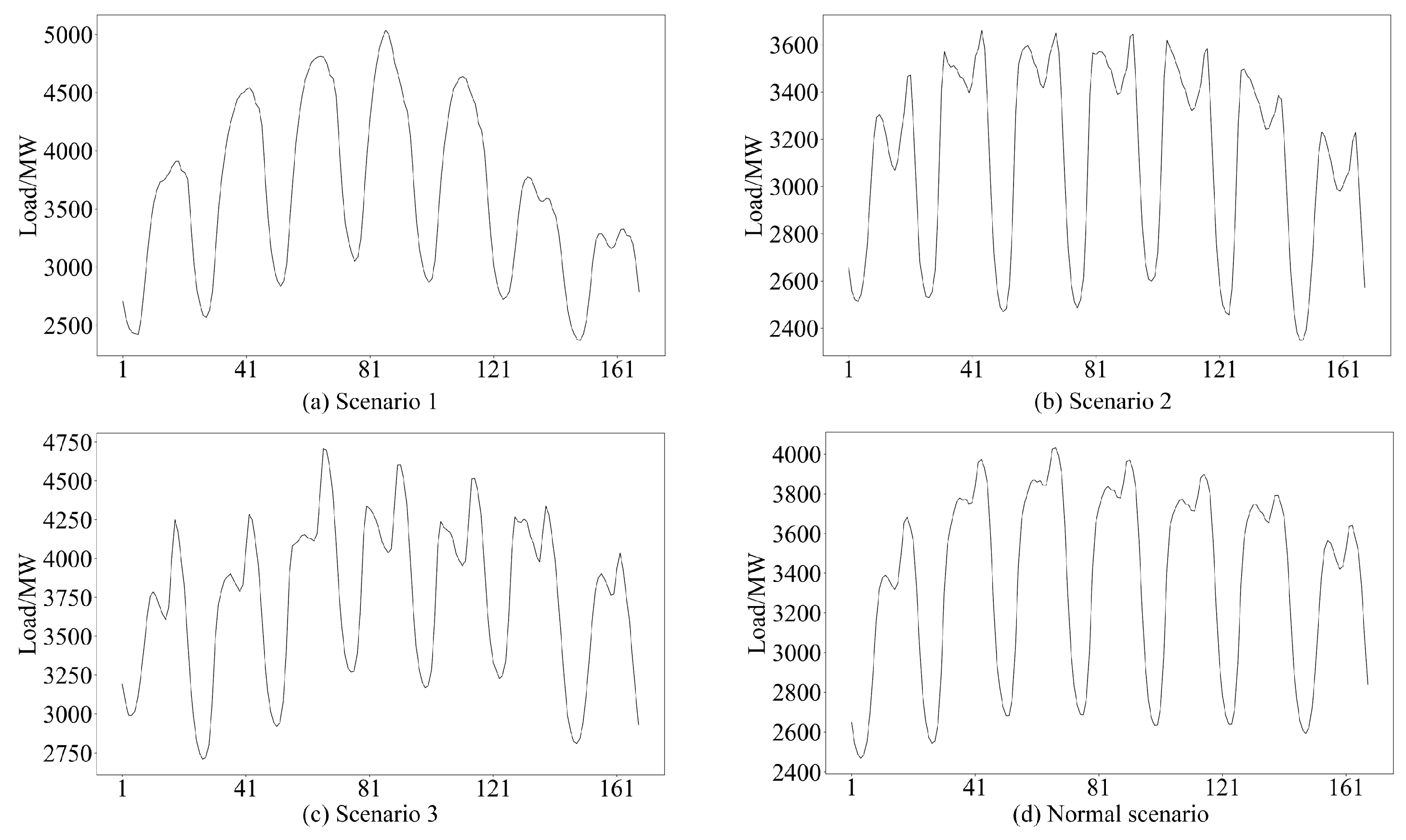
In this section, the fluctuation characteristics of extreme scenarios are analyzed in more detail. As noted in [8], extreme scenarios are defined by abnormal load fluctuations when compared to normal scenarios. To facilitate a clear comparison, a chart based on the DBSCAN extraction results is presented. Figure 4 includes subfigures (a), (b), and (c), which show several extreme scenarios identified by the proposed method, while subfigure (d) displays the average load data for the first 50 weeks of the year. By analyzing the average hourly load during this period, a clear cyclical pattern is observed, which helps reduce the impact of occasional fluctuations, thereby defining this as the normal scenario. Among the extreme scenarios, Scenario 1 exhibits the largest fluctuation amplitude, an irregular shape, and a significant peak-to-valley difference. Scenario 2, while showing a smaller fluctuation amplitude, has a higher frequency of changes, indicating more frequent shifts in power demand. Scenario 3, positioned between the other two, displays a larger fluctuation amplitude with some irregularity. These differences highlight the clear distinction between extreme and normal scenarios. Overall, the load fluctuations in extreme scenarios differ notably from those in normal conditions.

Figure 4.
Some extreme scenarios extracted by the proposed method.
3.2. Comparison Simulation
To evaluate the performance of the proposed model, three distinct extreme scenarios from the dataset, covering the periods of 5–11 January, 6–12 April, and 29 June–5 July 2014, were selected for comparison against LSTM, GRU, and Transformer models. The results are shown in Table 2.
Table 2.
Indicators for different forecasting models in different scenarios.
In Scenario 1, the RMSE of the proposed model is 32.547, which is 42.41% lower than LSTM’s 56.519, 37.13% lower than GRU’s 51.767, and 65.98% lower than the Transformer’s 95.670. The MAE is 23.260, 44.79% lower than LSTM’s 42.133, 39.44% lower than GRU’s 38.409, and 68.97% lower than the Transformer’s 74.969.
In Scenario 2, the RMSE of the proposed model is 35.117, showing a 40.05% improvement over LSTM’s 58.577, a 29.61% reduction compared to GRU’s 49.887, and a 50.21% decrease compared to the Transformer’s 70.529. The MAE is 26.460, 44.38% lower than LSTM’s 47.577, 33.62% lower than GRU’s 39.863, and 50.85% lower than the Transformer’s 53.835.
In Scenario 3, the RMSE is 36.871, 54.26% lower than LSTM’s 80.605, 39.65% lower than GRU’s 61.092, and 54.75% lower than the Transformer’s 81.477. The MAE is 29.175, 52.68% lower than LSTM’s 61.650, 35.94% lower than GRU’s 45.540, and 51.69% lower than the Transformer’s 60.390.
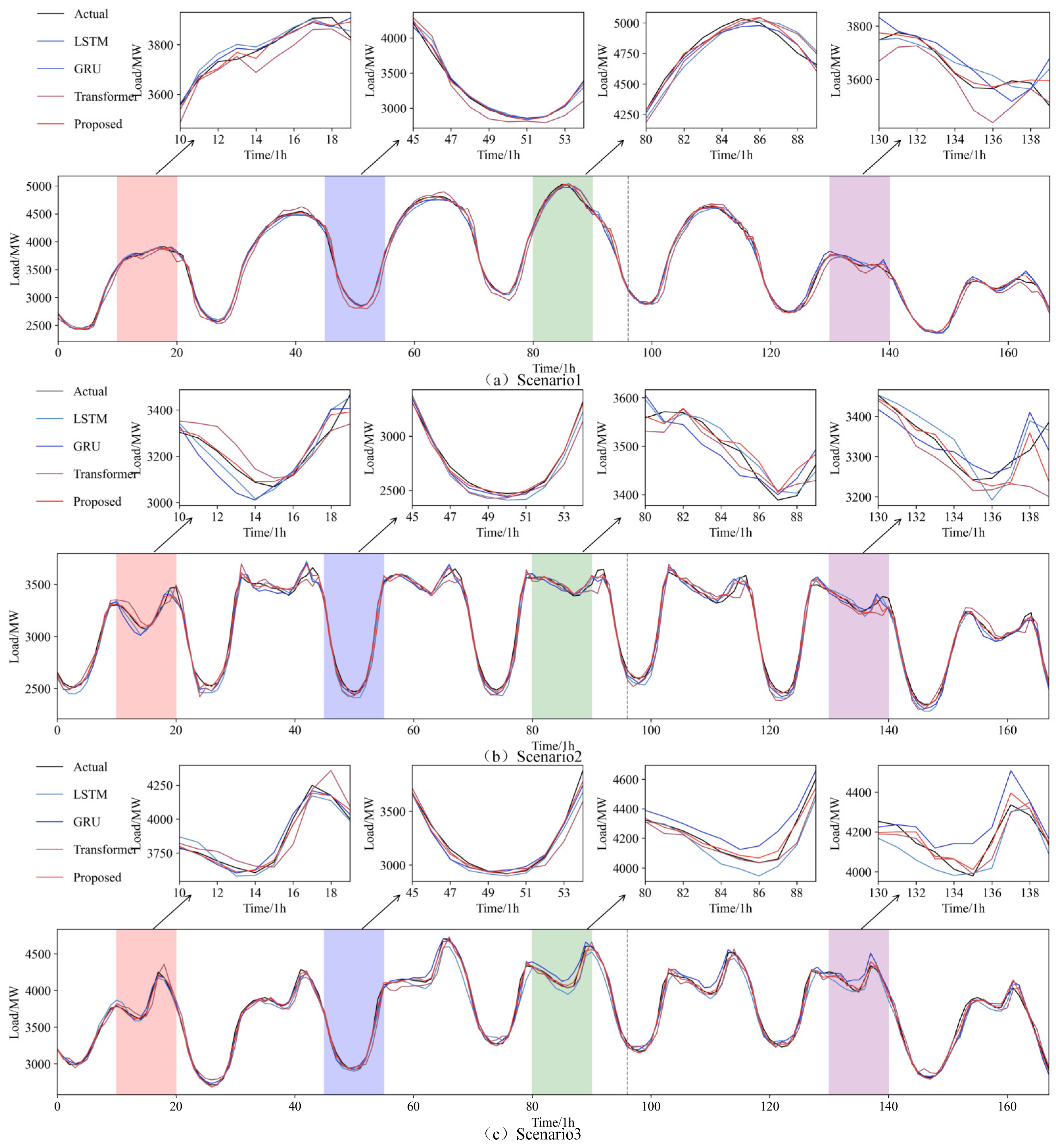
These results demonstrate the effectiveness of the fine-tuned RSBO-BiGRU-KNN-Attention model in improving load forecasting accuracy under extreme scenarios. Compared to the LSTM, GRU, and Transformer models, the BiGRU component, by capturing dependencies in both the forward and backward directions of the input sequence, enhances the model’s ability to detect complex nonlinear patterns. The custom KNN-Attention mechanism, which prioritizes the most relevant time steps and features, further improves forecasting performance. Freezing pre-trained weights and fine-tuning only the final layer helps prevent overfitting, ensuring the model remains adaptable in extreme scenarios. This results in substantial reductions in both RMSE and MAE, highlighting the model’s increased accuracy and stability.
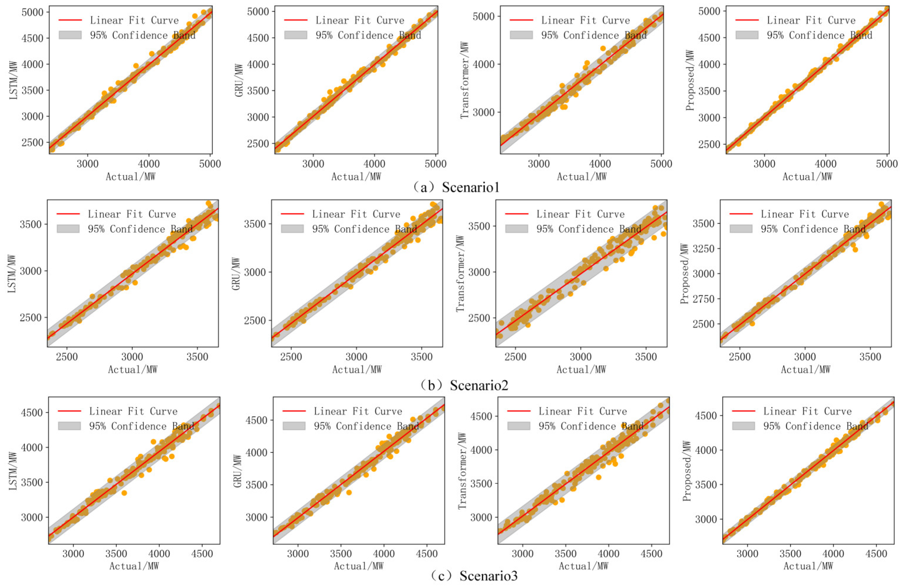
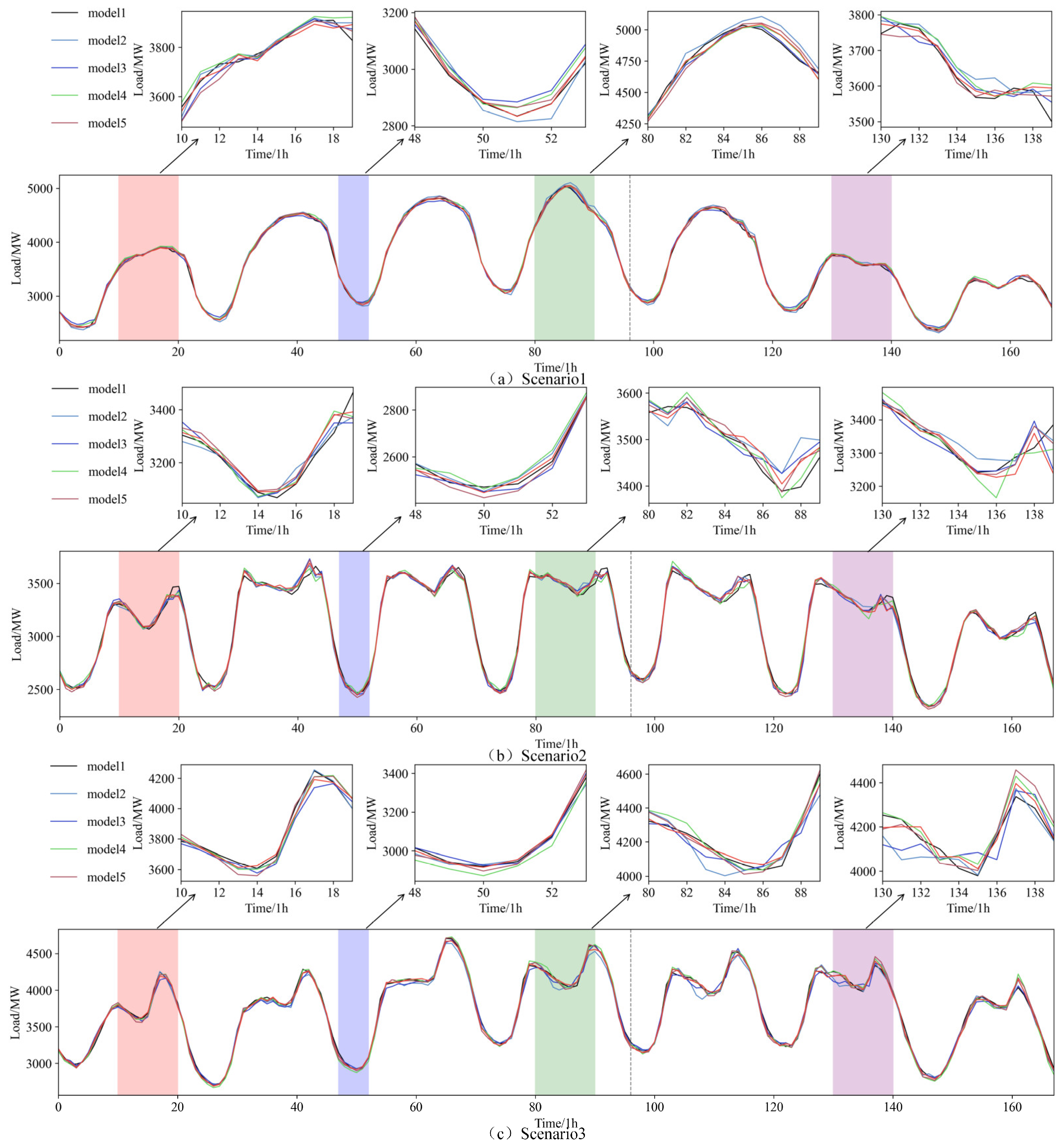
Figure 5 shows the forecasting curves, where the proposed model demonstrates superior forecasting accuracy during periods of significant load fluctuations, closely aligning with actual load data and outperforming the other models. Figure 6 displays scatter plots of the forecasted versus actual values for each scenario, with each subplot featuring a linear fit curve and a 95% confidence interval. The red line represents the fitted curve, while the gray shaded area indicates the confidence band. The yellow scatter points illustrate the distribution of actual and forecasted values. These plots reveal that the proposed model performs optimally in all scenarios, with the forecasted values tightly aligning with the actual values and the narrowest confidence interval, further proving its ability to capture underlying data patterns and improve forecasting accuracy.
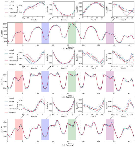
Figure 5.
Forecasting results of different models in different scenarios.
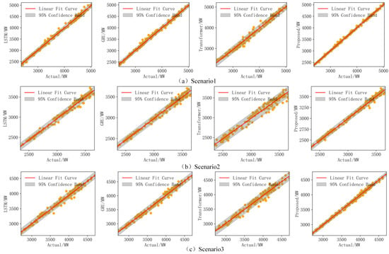
Figure 6.
Scatter plots of different models in different scenarios.
3.3. Ablation Study
To evaluate the contribution of each module to model performance, five configurations were considered: BiGRU (Model 1), BiGRU-Attention (Model 2), BiGRU-KNN-Attention (Model 3), RSBO-BiGRU-KNN-Attention (Model 4), and fine-tuned RSBO-BiGRU-KNN-Attention (Model 5). Comparative experiments were conducted across three extreme scenarios from the GEFCom2014 dataset, with the results presented in Table 3.
Table 3.
Indicators for ablation experiment.
The ablation study results show that the KNN-Attention module effectively reduces noise and enhances forecasting accuracy under extreme conditions. For example, in Scenario 1, the introduction of KNN-Attention leads to a 12.18% reduction in RMSE and an 11.84% reduction in MAE compared to Model 1. Furthermore, KNN-Attention provides a distinct advantage over the standard attention mechanism in extreme scenarios. Specifically, RMSE decreases by 5.35%, 8.73%, and 7.06% in the three scenarios, respectively.
The integration of RSBO allows the model to automatically search for optimal hyperparameters, improving performance across varying scenarios. In Scenario 3, for instance, RSBO reduces RMSE by 4.68% and MAE by 7.24%, demonstrating its effectiveness in adapting to extreme conditions.
The most notable improvement comes from the fine-tuning strategy, which significantly enhances model accuracy in all scenarios. Fine-tuning involves freezing most of the pre-trained model parameters and adjusting only the final fully connected layer, preventing large-scale parameter updates and maintaining stability. This is particularly beneficial in extreme scenarios with abnormal data distributions. Following fine-tuning, RMSE is reduced by over 14.91%, 8.81%, and 16.54% in the three scenarios, respectively, indicating that fine-tuning improves the model’s ability to handle noisy data and large fluctuations.
The results, as shown in Figure 7, further confirm that integrating the fine-tuning strategy leads to optimal performance across all scenarios. Notably, during periods of significant load peaks, the model’s forecasts align more closely with the actual load values.
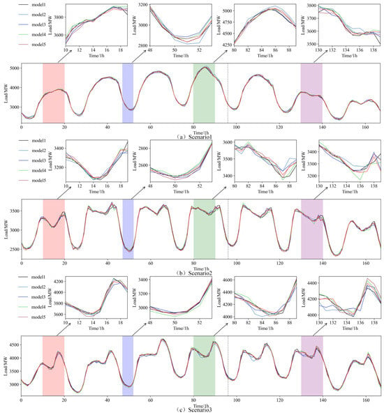
Figure 7.
Results of ablation study.
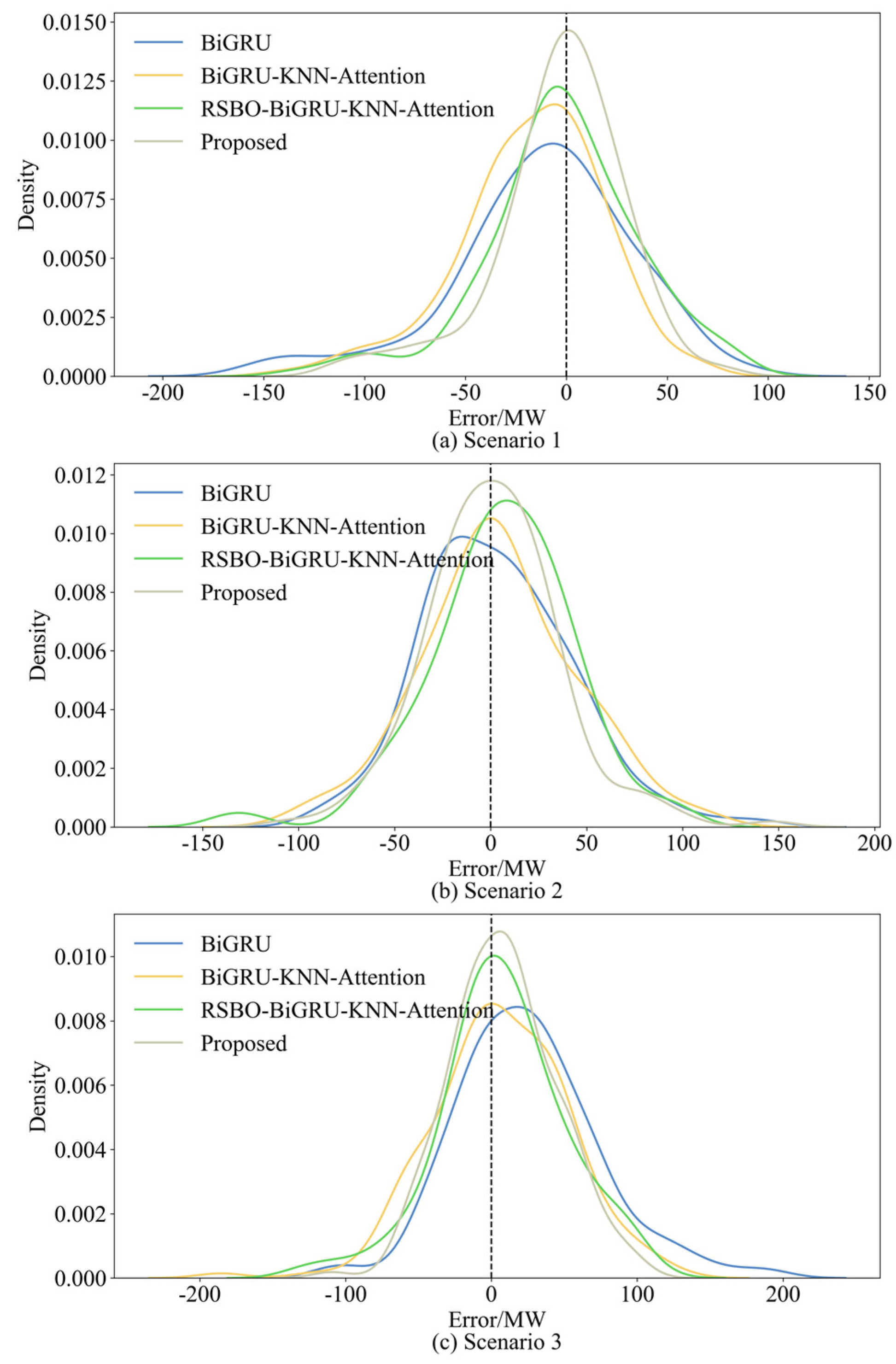
The error distribution chart visually compares the forecasting performance of different models by plotting the probability density function of errors between the predicted and actual values. A more concentrated error distribution around zero and a higher peak indicate better forecasting accuracy. Figure 8 shows the error distribution for several models under three distinct scenarios: BiGRU, BiGRU-KNN-Attention, RSBO-BiGRU-KNN-Attention, and the proposed model.
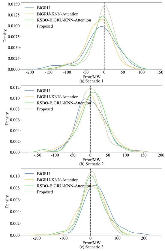
Figure 8.
Forecasting error distribution of different models in different scenarios.
From Figure 8, it is evident that the error distribution of the proposed model is the most concentrated across all scenarios, with the highest peak and the narrowest width. This suggests that its forecasting errors are smaller and more stable. In contrast, the error distributions of the other models are more spread out, with significant dispersion, particularly at the tails of the error range. Notably, in both Scenario 1 and Scenario 3, the error distribution includes both negative and positive errors.
The advantages of the proposed model are primarily attributed to the KNN-Attention mechanism, which effectively captures important long-range dependencies through the high-weight dot product selection. Additionally, the fine-tuning strategy preserves the model’s general feature extraction capability by freezing the earlier layers and optimizing only the fully connected layer, allowing for rapid adaptation to specific tasks. These improvements enhance the model’s adaptability in extreme scenarios, providing strong evidence of its accuracy in complex load forecasting tasks.
3.4. Supplementary Case Study Analysis
To further validate the model’s generalizability, additional experiments were conducted using the load dataset from New South Wales, Australia. The dataset includes load and temperature data from 1 January 2006 to 31 December 2010, with a data resolution of 30 min, load in MW, and 30 min ahead load forecasts. Three extreme scenarios from 2010 were selected for comparative analysis: 8 January to 14 January, 22 January to 28 January, and 24 December to 30 December, with the results shown in Table 4. The experiments show that the proposed model effectively captures long-term dependencies by focusing on key features in the data, and optimizes model parameters using RSBO. Compared to the benchmark models, the proposed model improves by more than 12.61% in terms of RMSE across different scenarios. Therefore, the proposed model can achieve the best forecasting accuracy in different extreme scenarios, even when applied to datasets from different regions, compared to the benchmark model.
Table 4.
Indicators for different forecasting models in different scenarios.
4. Conclusions
Accurate load forecasting is crucial for maintaining grid stability and optimizing energy management, especially during extreme conditions. This paper proposed a hybrid forecasting model that integrated a fine-tuning strategy within the DBSCAN-RSBO-BiGRU-KNN-Attention framework to enhance forecasting accuracy in such scenarios. The case results showed that the RSBO algorithm effectively explored high-dimensional parameter spaces, leading to improved model performance. Additionally, the fine-tuning strategy boosted both accuracy and generalization under extreme conditions. Compared to conventional models such as LSTM, GRU, and Transformer, the fine-tuned RSBO-BiGRU-KNN-Attention model shows over a 10% improvement in accuracy, with a 12.37% reduction in RMSE and a 6.73% decrease in MAE. These results highlighted the model’s superior forecasting capabilities.
Although existing methods effectively identify extreme scenarios with unusual fluctuations, they still have limitations. Future work could incorporate additional external factors, such as time-related features, climate changes, and equipment status, to better capture and analyze extreme conditions. The integration of these multidimensional features will further enhance the model’s ability to accurately extract and optimize extreme scenario forecasting.
Author Contributions
All authors contributed to this paper. All authors reviewed the manuscript. The work of each author is as follows: L.W.: Conceptualization, data curation, formal analysis, investigation, methodology, validation, visualization, writing—original draft. J.L. (Jifeng Liang): Conceptualization, formal analysis, investigation, methodology, project administration, supervision, writing—review and editing. J.L. (Jiawen Li): Conceptualization, supervision, writing—review and editing. Y.S.: Conceptualization, supervision, writing—review and editing. H.T.: Conceptualization, supervision, writing—review and editing. Q.W.: Conceptualization, supervision, writing—review and editing. T.Y.: Conceptualization, supervision, writing—review and editing. All authors have read and agreed to the published version of the manuscript.
Funding
This work was funded by the Science and Technology Project of State Grid Corporation of China under Grant No. 5108-202218280A-2-299-XG.
Data Availability Statement
The original contributions presented in this study are included in the article. Further inquiries can be directed to the corresponding author.
Conflicts of Interest
Authors Leibao Wang, Jifeng Liang, Qiang Wang, Tengkai Yu were employed by the company Electric Power Research Institute, State Grid Hebei Electric Power Co., Ltd. Author Hongzhu Tao was employed by the company National Power Dispatching and Control Center, State Grid Corporation of China. The remaining authors declare that the research was conducted in the absence of any commercial or financial relationships that could be construed as a potential conflict of interest. The companies had no role in the design of the study; in the collection, analyses, or interpretation of data; in the writing of the manuscript, or in the decision to publish the results.
References
- Zhang, Y.; Wang, J.; Sun, J.; Sun, R.; Qin, D. Power load forecasting system of iron and steel enterprises based on deep kernel–multiple kernel joint learning. Processes 2025, 13, 584. [Google Scholar] [CrossRef]
- Cui, J.; Kuang, W.; Geng, K.; Bi, A.; Bi, F.; Zheng, X.; Lin, C. Advanced short-term load forecasting with XGBoost-RF feature selection and CNN-GRU. Processes 2024, 12, 2466. [Google Scholar] [CrossRef]
- Wang, S.; Zhang, W.; Sun, Y.; Trivedi, A.; Chung, C.; Srinivasan, D. Wind power forecasting in the presence of data scarcity: A very short-term conditional probabilistic modeling framework. Energy 2024, 291, 130305. [Google Scholar] [CrossRef]
- Zimmermann, M.; Ziel, F. Efficient mid-term forecasting of hourly electricity load using generalized additive models. Appl. Energy 2025, 388, 125444. [Google Scholar] [CrossRef]
- Shah, S.A.H.; Ahmed, U.; Bilal, M.; Khan, A.R.; Razzaq, S.; Aziz, I.; Mahmood, A. Improved electric load forecasting using quantile long short-term memory network with dual attention mechanism. Energy Rep. 2025, 13, 2343–2353. [Google Scholar] [CrossRef]
- Yeganefar, A.; Amin-Naseri, M.R.; Sheikh-El-Eslami, M.K. Improvement of representative days selection in power system planning by incorporating the extreme days of the net load to take account of the variability and intermittency of renewable resources. Appl. Energy 2020, 272, 115224. [Google Scholar] [CrossRef]
- Zhu, X.; Yu, Z.; Liu, X. Security constrained unit commitment with extreme wind scenarios. J. Mod. Power Syst. Clean Energy 2020, 8, 464–472. [Google Scholar] [CrossRef]
- Xiaoxuan, X.; Dunwei, G.; Xiaoyan, S.; Yong, Z.; Rui, L. Short-term load forecasting of integrated energy system based on reconstruction error and extreme patterns recognition. Proc. CSEE 2022, 44, 3476–3488. [Google Scholar]
- Son, J.; Cha, J.; Kim, H.; Wi, Y.-M. Day-ahead short-term load forecasting for holidays based on modification of similar days’ load profiles. IEEE Access 2022, 10, 17864–17880. [Google Scholar] [CrossRef]
- Yuan, C.; Wang, S.; Sun, Y.; Wu, Y.; Xie, D. Ultra-short-term forecasting of wind power based on dual derivation of hybrid features and error correction. Autom. Electr. Power Syst. 2024, 48, 68–76. [Google Scholar]
- Tang, Y.; Lin, D.; Ni, C.; Zhao, B. XGBoost based bi-layer collaborative real-time calibration for ultra-short-term photovoltaic forecasting. Autom. Electr. Power Syst. 2021, 45, 18–27. [Google Scholar]
- Wang, Q.; Wang, Y.; Zhang, K.; Liu, Y.; Qiang, W.; Han Wen, Q. Artificial intelligent power forecasting for wind farm based on multi-source data fusion. Processes 2023, 11, 1429. [Google Scholar] [CrossRef]
- Ferreira, A.B.A.; Leite, J.B.; Salvadeo, D.H.P. Power substation load forecasting using interpretable transformer-based temporal fusion neural networks. Electr. Power Syst. Res. 2025, 238, 111169. [Google Scholar] [CrossRef]
- Wang, Y.; Sun, Y.; Li, Y.; Feng, C.; Chen, P. Interval forecasting method of aggregate output for multiple wind farms using LSTM networks and time-varying regular vine copulas. Processes 2023, 11, 1530. [Google Scholar] [CrossRef]
- Niu, D.; Yu, M.; Sun, L.; Gao, T.; Wang, K. Short-term multi-energy load forecasting for integrated energy systems based on CNN-BiGRU optimized by attention mechanism. Appl. Energy 2022, 313, 118801. [Google Scholar] [CrossRef]
- Wang, P.; Wang, X.; Wang, F.; Lin, M.; Chang, S.; Li, H.; Jin, R. Kvt: k-nn attention for boosting vision transformers. In Proceedings of the European Conference on Computer Vision, Tel Aviv, Israel, 23–27 October 2022; pp. 285–302. [Google Scholar]
- Upadhyay, R.; Phlypo, R.; Saini, R.; Liwicki, M. Sharing to learn and learning to share; fitting together meta, multi-task, and transfer learning: A meta review. IEEE Access 2024, 12, 148553–148576. [Google Scholar] [CrossRef]
- Cheng, K.; Peng, X.; Xu, Q.; Wang, B.; Liu, C.; Che, J. Short-term wind power forecasting based on feature selection and multi-level deep transfer learning. High Volt. Eng. 2022, 48, 497–503. [Google Scholar]
- Yin, H.; Ou, Z.; Fu, J.; Cai, Y.; Chen, S.; Meng, A. A novel transfer learning approach for wind power forecasting based on a serio-parallel deep learning architecture. Energy 2021, 234, 121271. [Google Scholar] [CrossRef]
- Zhang, C.; Zhang, F.; Gou, F.; Cao, W. Study on short-term electricity load forecasting based on the modified simplex approach sparrow search algorithm mixed with a bidirectional long- and short-term memory network. Processes 2024, 12, 1796. [Google Scholar] [CrossRef]
- Kottath, R.; Singh, P. Influencer buddy optimization: Algorithm and its application to electricity load and price forecasting problem. Energy 2023, 263, 125641. [Google Scholar] [CrossRef]
- Han, X.; Gao, Y.; Chen, Z.; Chen, Q.; Dong, X.; Sun, Y. An extreme scenario reduction algorithm for multi-time scale net-load. In Proceedings of the 2023 IEEE 7th Conference on Energy Internet and Energy System Integration (EI2), Hangzhou, China, 15–18 December 2023; pp. 225–230. [Google Scholar]
- Granell, R.; Axon, C.J.; Wallom, D.C.H. Impacts of raw data temporal resolution using selected clustering methods on residential electricity load profiles. IEEE Trans. Power Syst. 2014, 30, 3217–3224. [Google Scholar] [CrossRef]
- Hu, M.; Ge, D.; Telford, R.; Stephen, B.; Wallom, D.C.H. Classification and characterization of intra-day load curves of PV and non-PV households using interpretable feature extraction and feature-based clustering. Sustain. Cities Soc. 2021, 75, 103380. [Google Scholar] [CrossRef]
- Guo, H.; Chen, L.; Zhang, Q.; Huang, H.; Ma, Q.; Wang, J. Research and response to extreme scenarios in new power system: A review from perspective of electricity and power balance. Power Syst. Technol. 2024, 48, 3975–3991. [Google Scholar]
Disclaimer/Publisher’s Note: The statements, opinions and data contained in all publications are solely those of the individual author(s) and contributor(s) and not of MDPI and/or the editor(s). MDPI and/or the editor(s) disclaim responsibility for any injury to people or property resulting from any ideas, methods, instructions or products referred to in the content. |
© 2025 by the authors. Licensee MDPI, Basel, Switzerland. This article is an open access article distributed under the terms and conditions of the Creative Commons Attribution (CC BY) license (https://creativecommons.org/licenses/by/4.0/).