Abstract
The oil field enters a low-production liquid and high-water-cut stage, where the oil–water two-phase flow becomes increasingly complex and diverse. Traditional production profile logging interpretation methods often face significant errors and limitations. To improve interpretation accuracy, this study begins by examining the impact of flow rate and water cut on the oil–water two-phase flow pattern (defined as the characteristic distribution and movement of oil and water phases in the flow, which varies depending on flow conditions such as flow rate and water cut) through numerical simulations and surface experimental observations. The flow characteristics of the oil–water two-phase flow are clarified. Next, the data from surface experiments are collected using a multi-component logging tool, and artificial intelligence algorithms are employed to identify flow patterns and provide data support for production profile interpretation. The genetic algorithm–backpropagation (GA-BP) algorithm is used for flow type classification, with the flow pattern recognition accuracy reaching 93.75% when compared to the experimental results. Finally, the surface experimental data and flow patterns are input into the grey wolf and falcon optimization algorithm–radial basis function (GHOA-RBF) algorithm for training and prediction. The results show that the GHOA-RBF algorithm, incorporating flow patterns, exhibits superior prediction accuracy. Specifically, the coefficient of determination (R2) for oil flow is 0.996, and for water flow, it is 0.993, outperforming traditional RBF neural networks and the GHOA-RBF algorithm without flow pattern incorporation. This demonstrates that this study provides new theoretical support for production profile logging interpretation, with significant practical implications. However, limitations include the reliance on experimental data, which may not fully capture all field conditions, and the computational efficiency of the algorithm, which may need optimization for large-scale applications.
1. Introduction
Production profile logging is a logging method used in oil and gas production wells to understand the oil and water production conditions of different producing layers. In the production of oil and gas fields, accurately measuring phase flow rates is of great importance for predicting output and ensuring production safety [1].
Existing oil fields have entered the high-water-cut phase, where the underground oil–water distribution is complex, there are many influencing factors, flow pattern identification is difficult, and water cut is hard to measure. The measurement of multiphase flow and phase hold-up is a pressing issue that needs to be solved in practical logging. A survey was conducted on the current status of oil–water two-phase water-cut measurement, flow pattern identification, and the interpretation methods of production profile logging.
The water cut in oil–water two-phase flow refers to the ratio of the area occupied by water to the cross-sectional area of the pipeline [2]. Water cut is an important monitoring parameter, as it helps distinguish the oil–water ratio in the well, understand the well’s production capacity, estimate crude oil production, identify the producing layers of oil and water, predict the development life of oil wells, evaluate the exploitation value of the oil reservoir, and provide timely and accurate information for resource evaluation and downhole operations. Water-cut meters are instruments used to measure the water cut in oil wells. The commonly used types of water-cut meters include capacitive water-cut meters [3,4,5], conductivity water-cut meters [6,7,8], low-energy water-cut meters [9,10], and microwave water-cut meters [11,12].
Multiphase flow refers to the flow of two or more phases of substances simultaneously present in a system, where at least one phase is discontinuous (e.g., bubbles, droplets, solid particles, etc.) [13]. In multiphase flow, the interaction between different phases leads to changes in both the macroscopic properties and microscopic structures of the fluid, making the flow complex, nonlinear, unsteady, multi-scale, and multiphase. The different flow patterns or flow regimes observed in multiphase flow are collectively referred to as flow patterns. Research on flow patterns is fundamental to production profile interpretation studies. Different flow patterns require different interpretation parameters, making the classification of flow patterns and the determination of flow pattern boundaries essential for accurate production profile interpretation.
In 1961, Govier et al. conducted an oil–water two-phase flow experiment using a vertical transparent pipe with a diameter of 26.37 mm and a length of 720.58 mm. They found that the flow pattern sequence in liquid–liquid and gas–liquid systems was the same, but due to differences in viscosity, density, and interfacial tension, the flow patterns in the two systems were significantly different [14]. Zavareh et al. used an inclined transparent pipe in an oil–water two-phase flow experiment and observed three distinct bubbly flow regimes, including bubbly flow, dispersed bubbly flow, and reverse bubbly flow [15]. Flores et al. observed six different oil–water two-phase flow patterns in a vertical upward pipe with a diameter of 50.8 mm, including water-in-oil dispersed flow, water-in-oil fine dispersed flow, water-in-oil slug flow, oil-in-water slug flow, oil-in-water dispersed flow, and oil-in-water fine dispersed flow [16]. Zhong Xingfu et al. conducted experiments using oil–water as the medium in a vertical upward pipe with an inner diameter of 28.4 mm and a length of 2.56 m. They discovered an annular flow pattern and studied the oil hold-up and related parameters at the oil–water interface, such as wave shape, wave speed, and wavelength. The results showed that in this flow pattern, all wavelengths were less than twice the pipe diameter [17]. Jin Ningde et al. established a theoretical equation for the propagation characteristics of oil–water two-phase flow waves in vertical upward pipes based on the motion wave theory. They determined that the transition flow pattern occurred when the water hold-up was between 0.20 and 0.60. They proposed new criteria for identifying oil–water two-phase flow patterns in vertical upward pipes [18]. In 2008, Li Yingwei et al. applied statistical theory, wavelet packet theory, and chaos theory in combination to analyze the electrical conductivity fluctuations of oil–water two-phase flow in a vertical upward pipe. They extracted a set of characteristic parameters reflecting the dynamic characteristics of the oil–water two-phase flow and used these parameters for flow pattern identification [19]. In 2011, Ma Keshui et al. used experimental data from Farrar and Lucas to establish a closed two-fluid model for the numerical simulation of oil–water two-phase dispersed flow in vertical pipes. The model accurately simulated the local phase hold-up and velocity distribution under turbulent conditions [20]. In 2012, Yao Qi conducted a comparative analysis of the fluid distribution and flow structure of oil–water two-phase flow under different flow rates and water-cut conditions, based on the results from Flores at the University of Tulsa and measurements from an impedance water-cut meter. They identified four flow patterns: water-in-oil dispersed flow, water-in-oil fine dispersed flow, water-in-oil slug flow, and oil-in-water slug flow [21]. In 2020, Yin Hongyi et al. conducted a dynamic experiment of oil–water two-phase flow in an organic glass pipe, discovering three typical oil–water two-phase flow patterns: slug flow, bubbly flow, and fine bubbly flow. The slug flow pattern occurred under conditions of a low oil–water mixture velocity and low water cut. As the oil–water mixture velocity increased, the turbulent energy of the water phase was large enough to break the oil slugs, resulting in a water-in-oil bubbly flow structure. A further increase in velocity caused the turbulent energy of the water phase to be sufficient to break the oil bubbles, changing the flow pattern to a water-in-oil fine bubbly flow [22]. From the above investigation of the status of oil–water two-phase flow patterns, it was found that oil–water two-phase flow can be divided into five flow patterns: water-in-oil bubbly flow, slug flow, water-in-oil fine bubbly flow, oil-in-water foam flow, and oil-in-water emulsion flow.
Production profile logging interpretation primarily aims to understand the dynamic production conditions of production wells, providing a comprehensive analysis of the products, total output, and phase production rates of each production layer [23]. It serves as the basis for developing oil field development plans. Currently, the comprehensive water cut of oil wells has reached around 90%, and there are significant differences in the degree of oil field development. Accurate dynamic logging data are essential. However, due to the limitations of current testing technologies and well conditions, production profile logging data are often difficult to record, which presents challenges for interpretation. Common methods for production profile logging interpretation include model-based interpretation methods [24,25] and experimental chart methods [26].
Low-production fluids, where the oil–water mixture velocity is low, result in severe slip effects of oil–water two-phase flow in vertical wells, leading to highly uneven phase distribution. High-water-cut conditions cause oil bubbles to become very small and lead to discontinuous oil flow. These complex and highly random flow characteristics present significant difficulties and challenges for production profile logging. Additionally, the flow in vertical wells with high water cuts is complex, and the instrument response is also intricate, further complicating the logging interpretation. Moreover, factors such as fluid density, viscosity, and phase hold-up are highly affected by flow patterns, temperature, and pressure [27], all of which make it difficult for conventional production profile logging interpretation methods to yield precise results.
Artificial intelligence (AI) technology can fully utilize large logging datasets, integrate expert knowledge, and automatically and intelligently interpret logging data. This approach can avoid the subjective judgments of human interpreters [28], which is crucial for improving the accuracy and precision of logging data interpretation.
To address the challenges of interpreting low-production fluids and high-water-cut oil–water two-phase flow in production profile logging, the approach begins with applying numerical simulation to study the flow characteristics of oil–water two-phase flow. This helps to further understand and monitor the flow characteristics in vertical wells, providing guidance for production logging experiments. Next, an oil–water two-phase ground simulation experiment is conducted to collect a large amount of logging data. These data will serve as the foundation for using AI algorithms to identify flow patterns in high-water-cut production wells. By combining on-site high-water-cut oil well production logging data and wellhead metering data, a set of sample points will be established to support the interpretation of high-water-cut oil–water two-phase production profiles. Finally, AI algorithms will be used to identify flow patterns in oil–water two-phase flow based on sample point data (including turbine speed, flow rate, water cut, etc.). Based on this flow pattern classification, AI algorithms will be applied to predict phase flow rates and interpret the production profile data. This methodology aims to explore new methods for interpreting high-water-cut oil–water two-phase production profile logging.
2. Numerical Simulation Study of Oil–Water Two-Phase Production Wells
Numerical simulation can quickly model changes in the flow field and the internal structure of fluids [29], without being constrained by geometric models or experimental environmental conditions. It is capable of calculating complex physical problems that are difficult to achieve in actual experimental processes. Through numerical simulation, the dynamic flow field in the production wellbore can also be modeled, allowing for the study of the flow variation in oil–water two-phase systems within the wellbore. This provides valuable reference data for the research of oil–water two-phase flow in real-world conditions.
Computational Fluid Dynamics (CFD) is a technique that uses numerical methods to simulate and solve fluid mechanics problems [30]. As an important research tool, CFD can be widely applied in related research fields, such as fluid flow, heat transfer, and molecular transport [31]. CFD simulation describes fluid motion through mathematical models, transforming fluid mechanics problems into numerical computation problems. By using computers to solve these mathematical models, CFD provides information on fluid flow states, mechanical properties, temperature distribution, pressure distribution, and other related aspects.
2.1. Simulation Conditions Setup
2.1.1. Geometric Model Creation and Mesh Generation
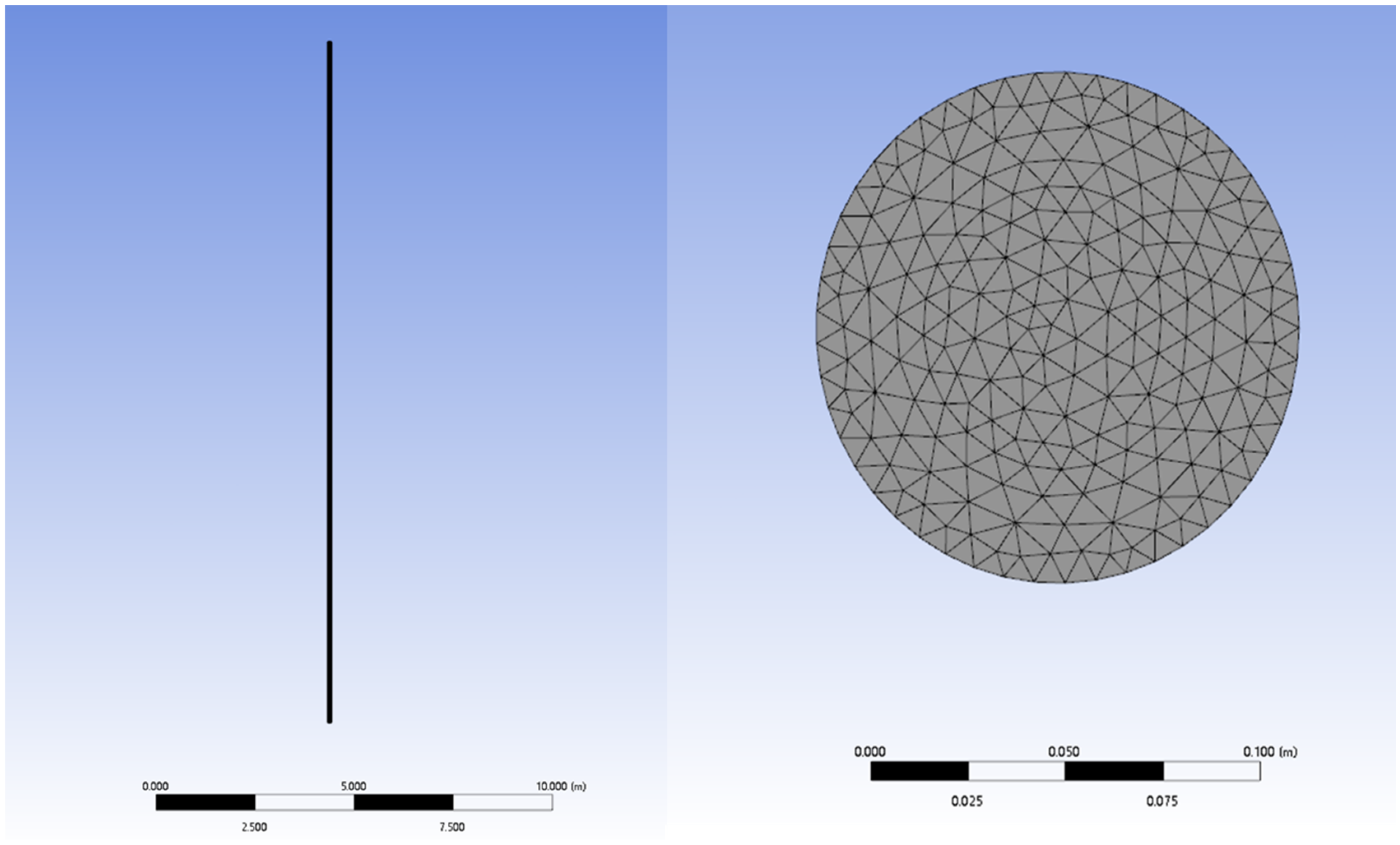
The CFD simulation was used to model the flow state of the oil–water two-phase flow within a vertical well. A geometrical model of the vertical wellbore was created with a 90° inclination angle. The internal diameter of the pipe was 124 mm, and the length of the pipe was 20 m. The inlet of the two-phase flow was located at the bottom of the model pipeline, and the outlet was at the top. The overall computational domain of the pipeline was 124 mm by 20,000 mm.
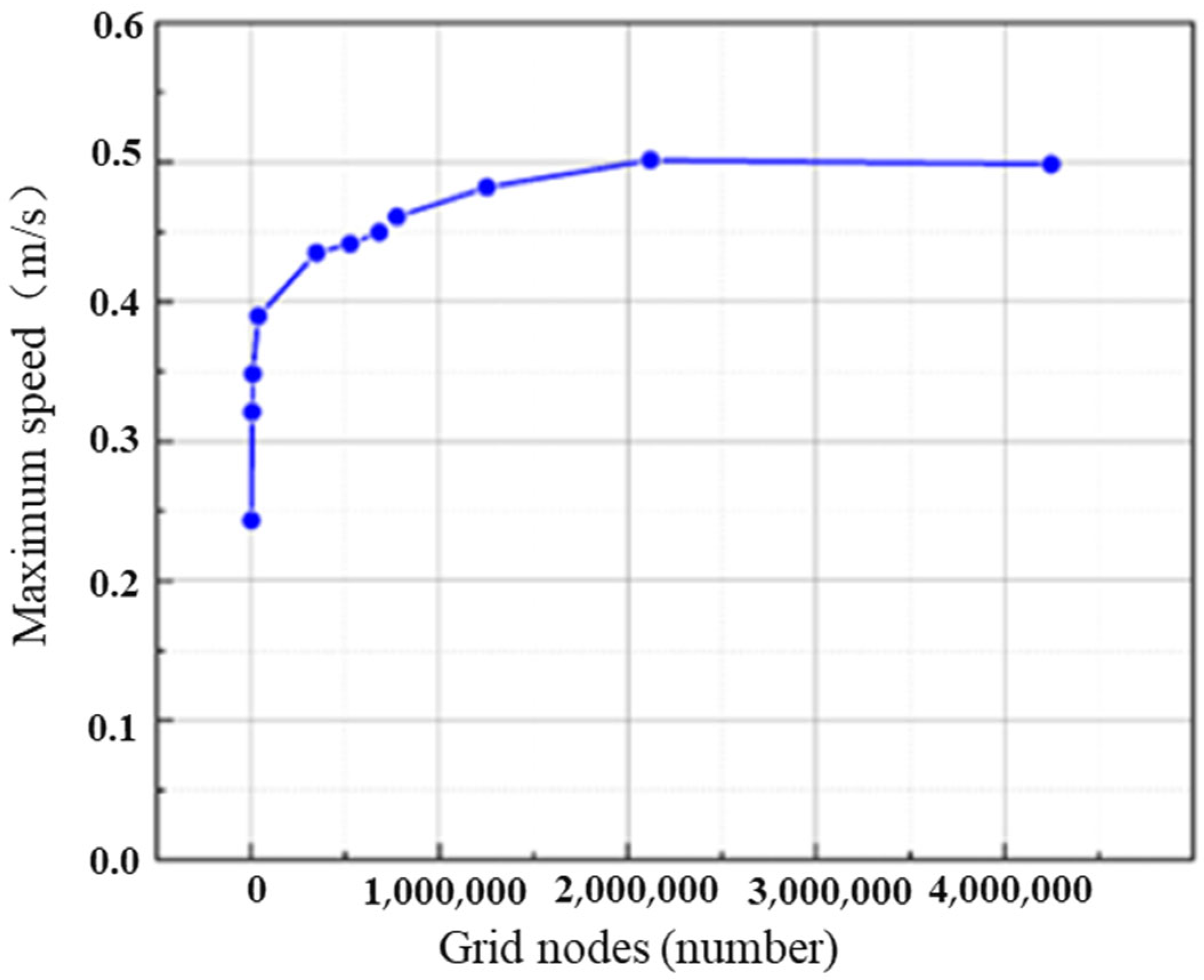
Since the mesh density has a significant impact on the accuracy and efficiency of simulation results, a larger mesh count requires more memory and longer computational time. Conversely, a smaller mesh count results in lower solution accuracy. Therefore, selecting an appropriate mesh count is crucial in the numerical simulation process. To verify mesh independence, the maximum velocity parameter at the wellbore pressure outlet boundary was compared and analyzed with varying mesh counts under the same simulation parameters. The specific parameters are shown in Table 1. As shown in Figure 1, the maximum velocity at the outlet boundary exhibits a trend of change with the increase in the mesh node count. When the mesh node count exceeds 2,088,428, the change in maximum velocity becomes gradual. This suggests that the current mesh count offers better computational efficiency compared to a finer mesh. Hence, this mesh count can be considered optimal for the calculation. Additionally, based on the mesh quality shown in Figure 2, a higher mesh quality value (closer to 1) indicates a better mesh. Therefore, a mesh with 2,088,428 nodes and 2,385,636 cells was selected, as shown in Figure 3.

Table 1.
Number of grid nodes and simulation parameters.

Figure 1.
Trend chart of maximum velocity at the exit of different grid nodes.
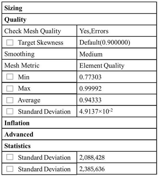
Figure 2.
Grid quality, grid nodes, and quantity.
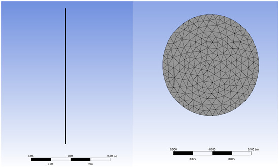
Figure 3.
Geometry model of the vertical wellbore and cross-section of the wellbore.
2.1.2. Simulation Settings and Boundary Conditions
To simulate two-phase oil–water flow, this study uses water and white oil as the fluid materials. These two fluids are considered incompressible, and their heat transfer is negligible. Since the flow of air and water is incompressible, fluid properties such as density and viscosity are not affected by temperature and pressure and are considered constant. The physical parameters of the fluid media used in the simulation are described in Table 2. The inlet boundary (at the bottom of the pipe) was selected as a velocity inlet boundary, while the outlet boundary (at the top of the pipe) was chosen as a pressure outlet boundary. The surrounding walls were treated as no-slip wall surfaces. A pressure solver was used for the transient simulations, and the environmental pressure was set to standard atmospheric pressure for the simulation [32].
Table 2.
Simulate the physical properties of fluid media.
ANSYS Fluent 2021 R2 software uses the Reynolds-averaged approach to establish a series of commonly used RANS models, including the standard k-ε model, RNG k-ε model, realizable k-ε model, k-ω model, and Reynolds stress model, among others. These turbulence models are modifications tailored to different practical applications and can generally solve most real-world turbulent flow problems. The detailed applicability of these flow models is shown in Table 3 below.
Table 3.
Applicability of turbulence models in FLUENT.
There is currently no universal turbulence model to explain turbulence scales. FLUENT software offers several turbulence models suitable for different flow conditions. This study addresses the oil–water two-phase flow problem, where turbulence occurs in situations involving smaller pipe diameters or lower flow velocities. In these cases, the Reynolds number for turbulence is relatively low, ranging from approximately 4000 to 10,000, which makes the widely used standard k-ε model for low Reynolds numbers more suitable for application [33].
2.2. Numerical Simulation Results and Analysis
Based on the previously established vertical wellbore geometry model, numerical simulations of the oil–water two-phase flow were conducted. The simulation results were processed to generate phase distribution maps of the fluid inside the wellbore and at the flow interface under different operating conditions, allowing for the analysis of the distribution characteristics of flow patterns under various conditions. Inside the vertical wellbore, by adjusting the oil–water two-phase flow rates and water cut, five typical flow patterns were obtained, as shown in the figure. In the figure, the red portion represents the water phase, and the blue portion represents the oil phase.
- Water-in-oil bubbly flow: Water is the continuous phase, and oil bubbles, varying in size, are dispersed throughout the wellbore, as shown in Figure 4.
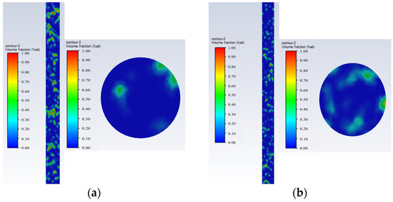 Figure 4. Water-in-oil bubbly flow oil–water phase distribution and cross-sectional view; they should be listed as follows: (a) Q = 50 m3/d, and water cut 80%; (b) Q = 100 m3/d, and water cut 80%.Figure 4. Water-in-oil bubbly flow oil–water phase distribution and cross-sectional view; they should be listed as follows: (a) Q = 50 m3/d, and water cut 80%; (b) Q = 100 m3/d, and water cut 80%.
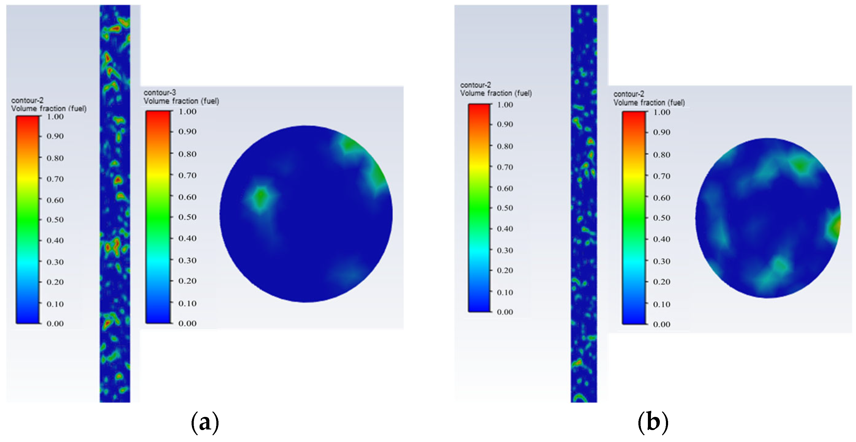
- Water-in-oil dispersed bubbly flow: Water is the continuous phase. The oil bubbles become smaller, denser, and uniformly dispersed in the water, filling the entire pipe and covering the entire cross-section of the pipe, as shown in Figure 5.
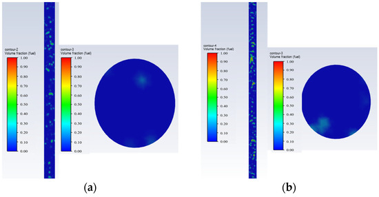 Figure 5. Water-in-oil dispersed bubbly flow oil–water phase distribution and cross-sectional view; they should be listed as follows: (a) Q = 25 m3/d, and water cut 95%; (b) Q = 50 m3/d, and water cut 95%.Figure 5. Water-in-oil dispersed bubbly flow oil–water phase distribution and cross-sectional view; they should be listed as follows: (a) Q = 25 m3/d, and water cut 95%; (b) Q = 50 m3/d, and water cut 95%.
- Pulsating bubbly flow: Water is the continuous phase. The oil bubbles rise intermittently in pulses, occupying the center of the pipe, and are clearly visible, as shown in Figure 6.
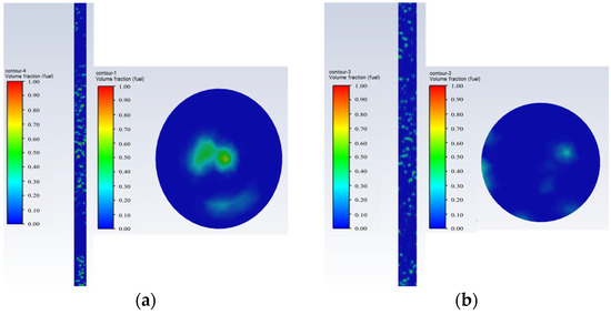 Figure 6. Pulsating bubbly flow oil–water phase distribution and cross-sectional view; they should be listed as follows: (a) Q = 5 m3/d, and water cut 80%; (b) Q = 5 m3/d, and water cut 80%.Figure 6. Pulsating bubbly flow oil–water phase distribution and cross-sectional view; they should be listed as follows: (a) Q = 5 m3/d, and water cut 80%; (b) Q = 5 m3/d, and water cut 80%.
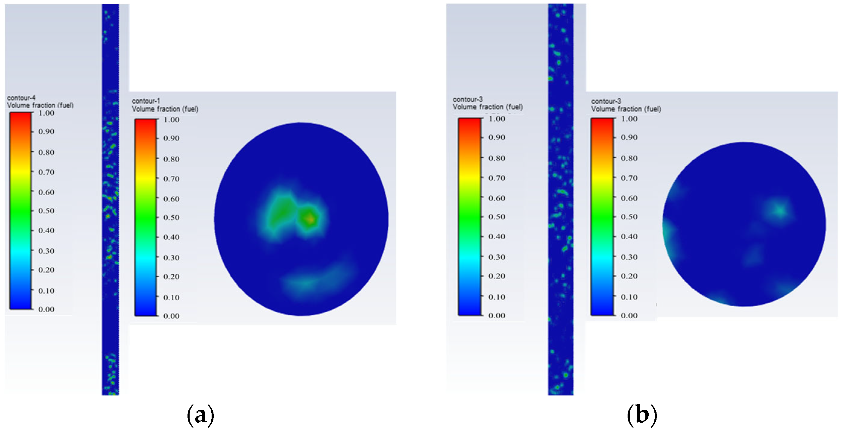
- Emulsified flow: Oil is the continuous phase, and water exists in the form of droplets that rise together with the oil, as shown in Figure 7.
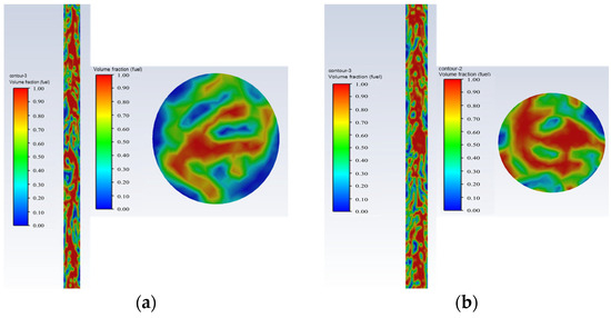 Figure 7. Emulsified flow oil–water phase distribution and cross-sectional view; they should be listed as follows: (a) Q = 503/d, and water cut 20%; (b) Q = 100 d, and water cut 20%.Figure 7. Emulsified flow oil–water phase distribution and cross-sectional view; they should be listed as follows: (a) Q = 503/d, and water cut 20%; (b) Q = 100 d, and water cut 20%.
- Oil-in-water bubbly flow: Oil is the continuous phase, and water bubbles are uniformly dispersed in the oil, filling the entire pipe and covering the entire cross-section of the pipe, as shown in Figure 8.
 Figure 8. Oil-in-water bubbly flow oil–water phase distribution and cross-sectional view; they should be listed as follows: (a) Q = 503/d, and water cut 5%; (b) Q = 100 d, and water cut 5%.Figure 8. Oil-in-water bubbly flow oil–water phase distribution and cross-sectional view; they should be listed as follows: (a) Q = 503/d, and water cut 5%; (b) Q = 100 d, and water cut 5%.
The results of the numerical simulation show that in a vertical wellbore with a diameter of 124 mm, under normal temperature and pressure conditions, the oil–water two-phase flow velocity ranges from 5 m3/d to 100 m3/d, and the water cut ranges from 5% to 95%. Five types of oil–water two-phase flow patterns were obtained through the numerical simulation. When the flow rate is between 10 m3/d and 50 m3/d and the water cut is 80% to 85%, the flow pattern is water-in-oil bubbly flow; when the flow rate is between 10 m3/d and 100 m3/d and the water cut is 95%, the flow pattern is dispersed bubbly flow; when the flow rate is between 5 m3/d and 10 m3/d and the water cut is 80% or 90%, the flow pattern is pulsating bubbly flow; when the flow rate is between 10 m3/d and 100 m3/d and the water cut is 20%, the flow pattern is emulsified flow; and when the flow rate is between 10 m3/d and 100 m3/d and the water cut is 5%, the flow pattern is oil-in-water bubbly flow. In summary, the numerical simulation calculation experiments can provide valuable guidance for oil–water two-phase production logging simulation testing experiments.
3. Ground Simulation Experiment Research
3.1. Experimental Setup and Experimental Plan
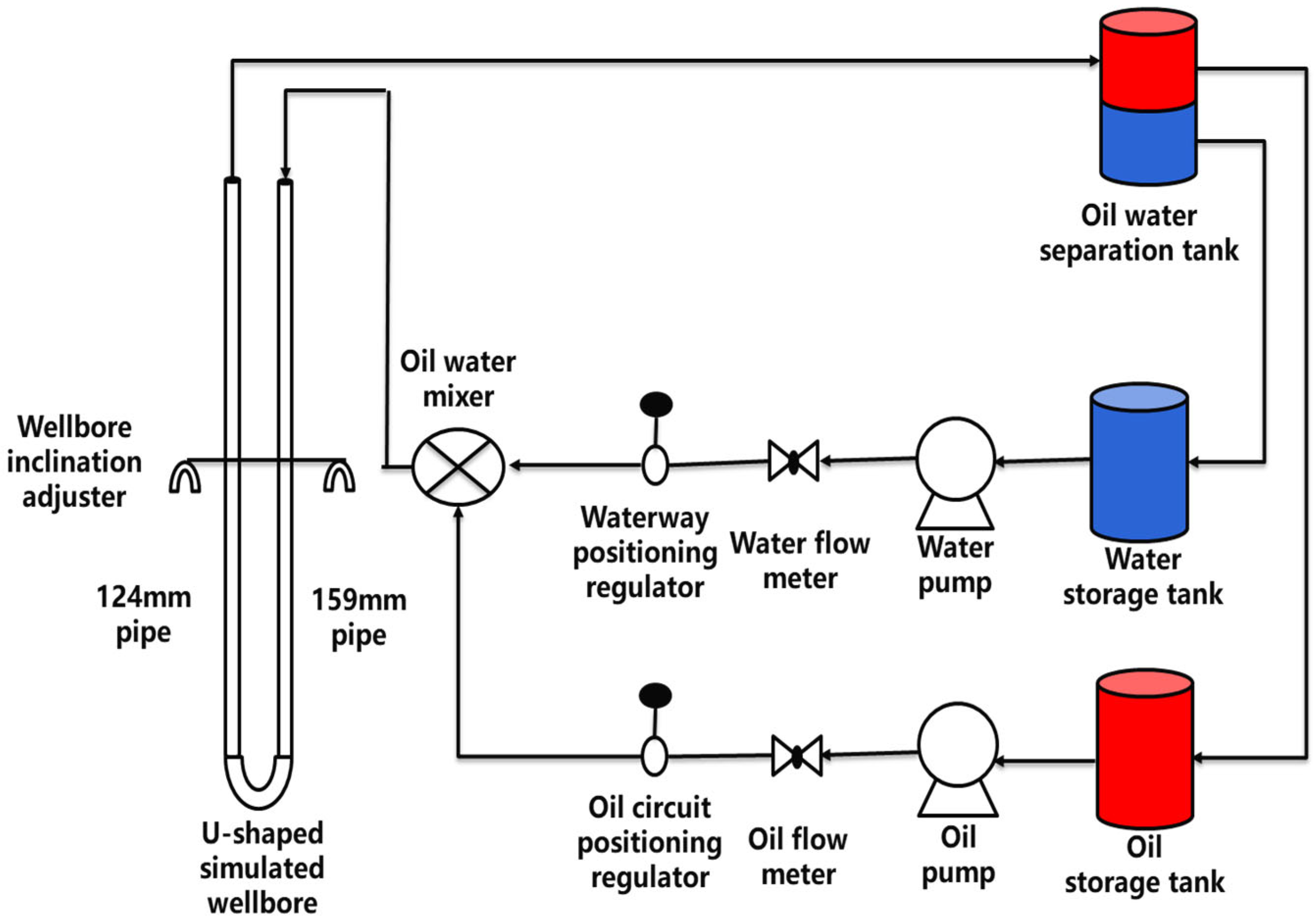
The ground oil–water two-phase flow dynamic simulation experiment was conducted on the multiphase flow simulation experimental platform for horizontal and highly inclined wells at Yangtze University. The working principle diagram of the experimental device is shown in Figure 9. The experimental platform’s wellbore height is 12 m, with two specifications for the wellbore diameter: 124 mm and 159 mm. The material used for the wellbore is transparent acrylic pipe. The two transparent pipes are installed on a fixed frame and connected to form a U-shaped pipeline. Each pipe is equipped with quick-closing solenoid valves at both the top and bottom to ensure that the fluid flow can be instantly stopped. A ruler with a scale of 1 mm is fixed between the two pipes, used to measure the hold-up by quickly closing the valves. The wellbore’s tilt angle is adjustable, ranging from horizontal to vertical, and is controlled by hydraulic drive. A manual switch is set up on the surface for operation. The liquid-phase flow rate on the experimental platform ranges from 0.2 to 600 m3/d, while the gas-phase flow rate ranges from 0.1 to 1000 m3/d. The gas- and liquid-phase fluids are delivered to the pressure stabilization tank by industrial-grade peristaltic pumps and then enter the metering pipeline, ensuring that the fluid flow in the transport pipeline is not affected by the pulsations of the delivery pumps [34].

Figure 9.
Schematic diagram of the multiphase flow simulation experimental device.
This experiment used traditional production logging tools, including a central turbine flowmeter and a capacitive water content meter. The sampling frequency of the instrument was 1 data point per second. The measured parameters included moisture content, mixing density, turbine speed, and other logging data. Sensors and data acquisition systems were used to monitor and record key parameters in real time during the process. Real-time monitoring of the flow inside the experimental wellbore was conducted using high-speed cameras.
The water hold-up meter used a capacitive principle to measure the water hold-up by exploiting the differences in the dielectric properties of oil, gas, and water (for example, the dielectric constant of water is 60–80, while that of oil and gas is 1–4). The principle was to convert the change in dielectric constant into a change in capacitance, which in turn caused a change in the oscillation circuit’s output frequency. Finally, the frequency value was converted into the downhole water hold-up percentage through the instrument’s calibration [35].
The flow meter was based on the principle of conservation of momentum and uses a turbine flow meter design. The fluid impacted the turbine blades, causing them to rotate, and the rotational speed was proportional to the flow rate. The turbine rotational speed was converted into electrical pulse signals through a magnetoelectric conversion device. The secondary instrument calculated and displayed the instantaneous flow rate and cumulative flow rate.
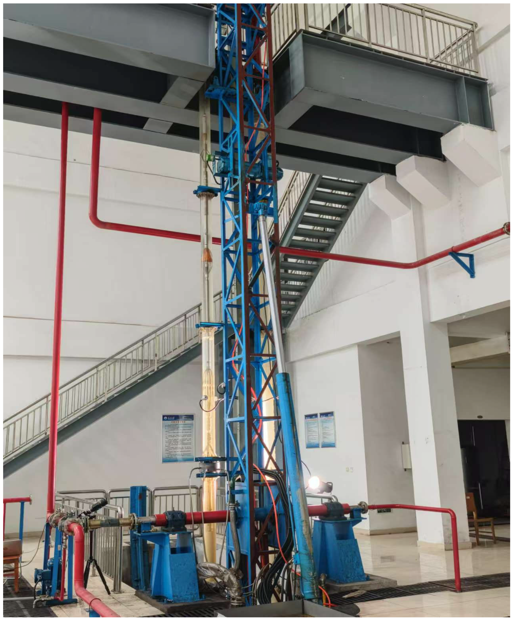
This experiment was conducted in a wellbore with an inner diameter of 124 mm and a wellbore angle of 90° (vertical wellbore, relative to the horizontal direction of the ground), as shown in Figure 10. The experimental fluid medium was No. 10 industrial white oil and tap water. The specific experimental fluid parameters and experimental plan are shown in Table 4. Different flow rates of oil and water were input according to the experimental plan. In order to ensure the full development of the fluid, after the oil–water flow ratio at each experimental point was stable, we waited for half an hour before turning on the instrument for measurement. During measurement, the instrument recorded the logging data such as the water holding count rate and turbine speed once per second. In order to reduce errors, the measurement time was 5 min, and a total of 300 data points were measured at each point. In order to verify the reproducibility of the experimental results, this study conducted multiple experiments under the same experimental conditions. Three repeated experiments were conducted under each experimental condition, and a statistical analysis was conducted on the measurement results of key variables, such as flow rate, moisture content, and instrument response values. The results indicated that the variability between different experiments was small, which verified the reliability and reproducibility of the experimental results. Therefore, we can confirm that the obtained data have high repeatability and can provide reliable basis for subsequent analysis.
Figure 10.
Ground simulation experiment site.
Table 4.
Fluid parameters and experimental plan.
3.2. Analysis of Experimental Results
Based on the two-phase oil–water flow type data from previous studies [36], a high-speed camera was used to record the phase distribution in the vertical pipeline (mainly observing the oil–water two-phase flow patterns). The oil–water two-phase distribution in the flow field varied under different flow rates, water-cut conditions, etc., resulting in different flow structures. The following flow patterns were identified through comparison.
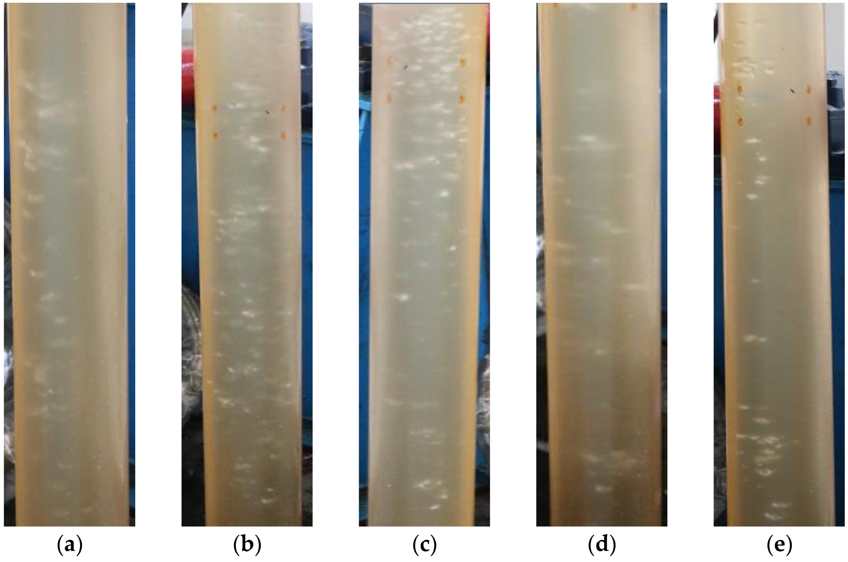
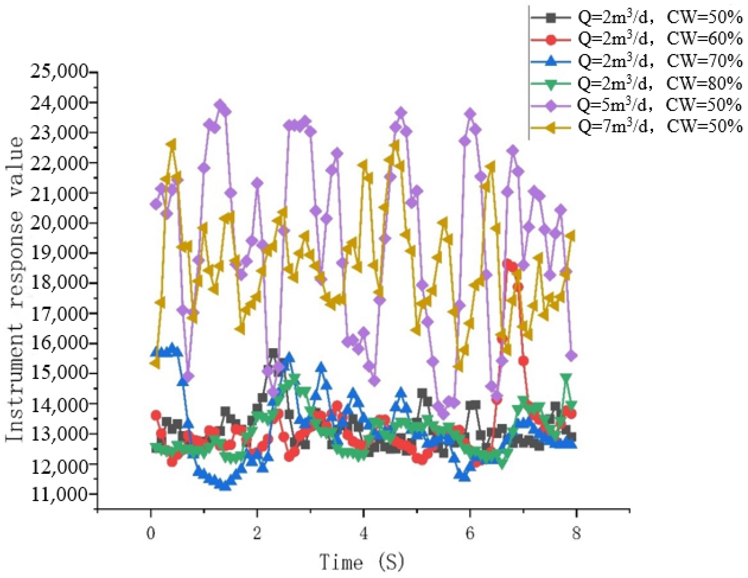
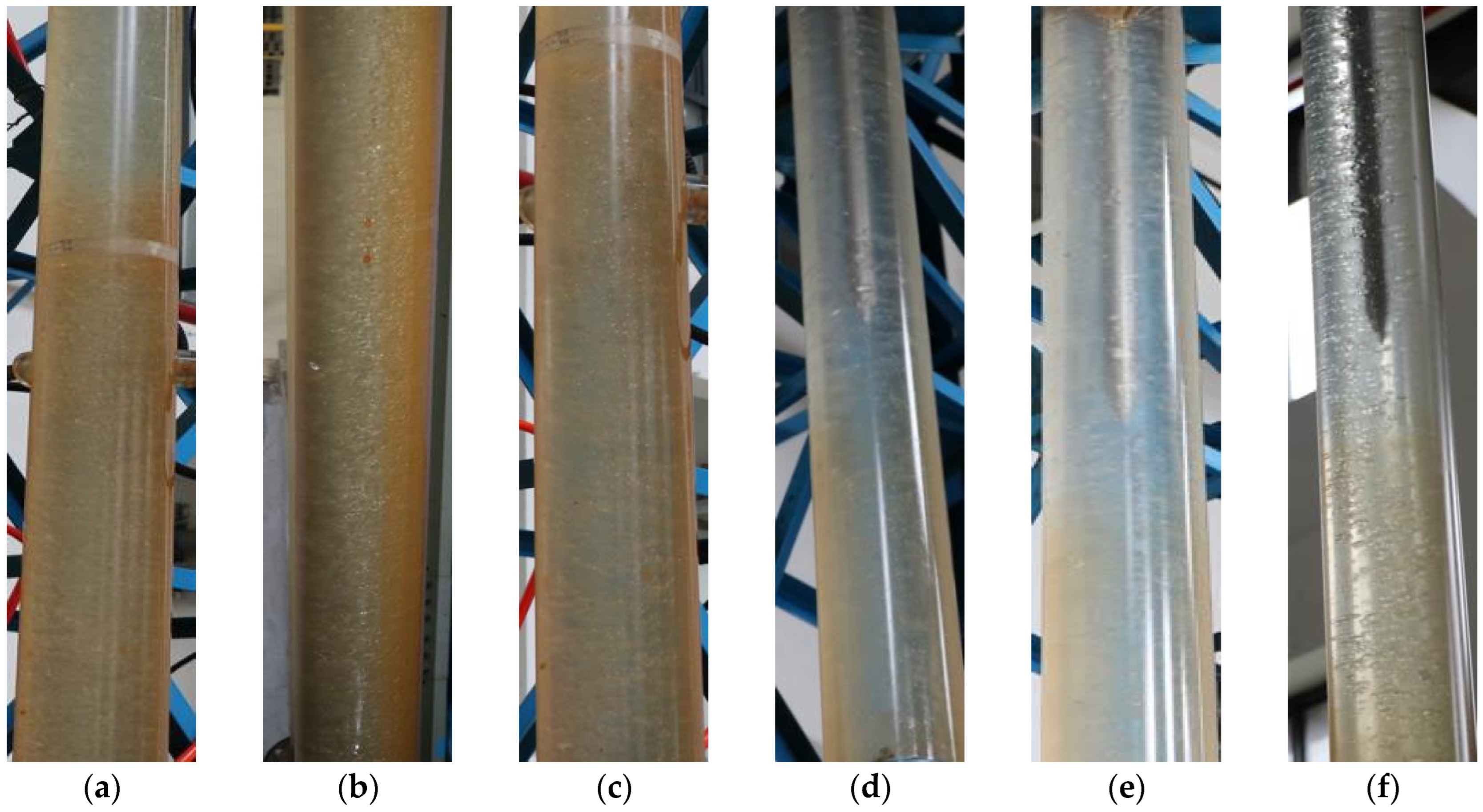
Bubble flow: Water becomes the continuous phase, with larger oil bubbles evenly and continuously dispersed in the water, moving at high speeds. As they rise, they carry liquid with them, and the interaction between the oil bubbles causes unstable flow. The corresponding pattern observed by the capacitance water-cut meter also indicates that, during bubble flow, the flow instability leads to significant fluctuations in the capacitance water-cut value, as shown in Figure 11 and Figure 12.
Figure 11.
Observed flow patterns in the ground simulation experiment. They should be listed as follows: (a) Q = 2 m3/d, and water cut 85%; (b) Q = 2 m3/d, and water cut 60%; (c) Q = 2 m3/d, and water cut 70%; (d) Q = 2 m3/d, and water cut 80%; and (e) Q = 10 m3/d, and water cut 85%.
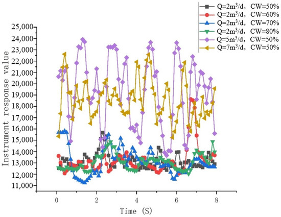
Figure 12.
Response graph of the capacitance water-cut meter over time.
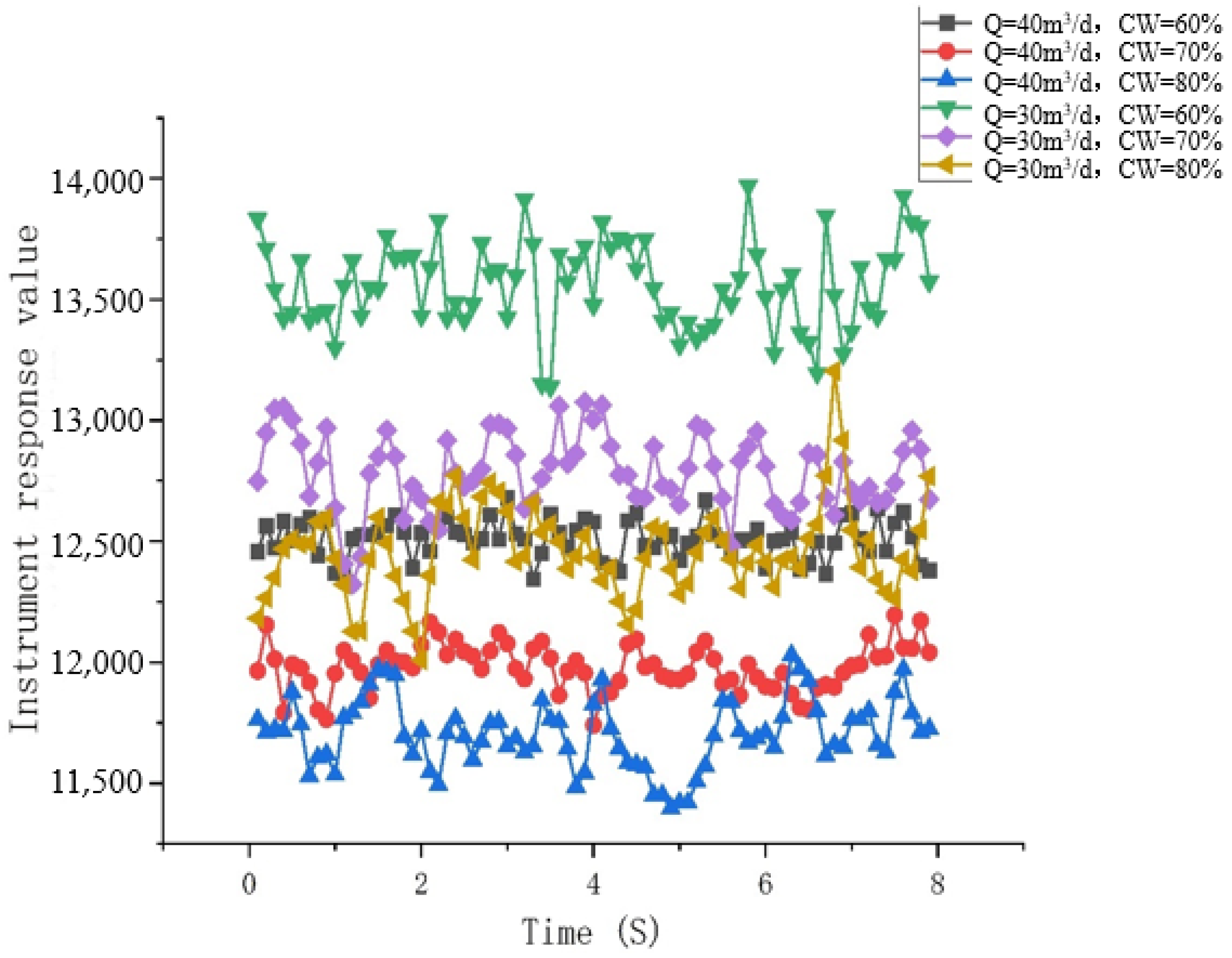
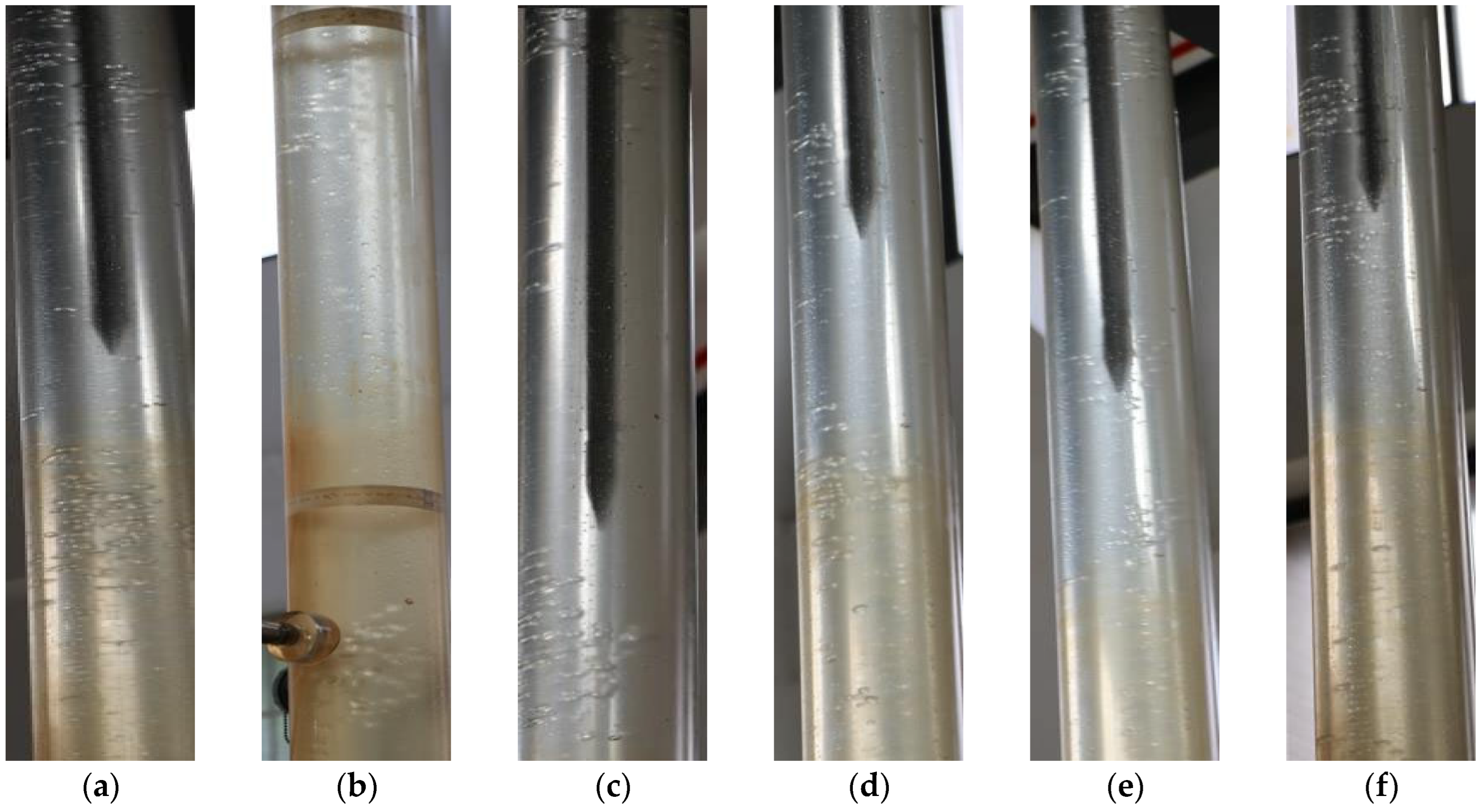
Fine bubble flow: Water is the continuous phase. The oil bubbles become smaller and more densely packed, uniformly dispersed in the water, filling the entire pipe and covering the entire pipe cross-section. The oil and water flow upward uniformly and stably. As observed from the capacitance water-cut meter, during fine bubble flow, the flow is stable and upward, which leads to a relatively steady change in the capacitance water-cut value over time, as shown in Figure 13 and Figure 14.
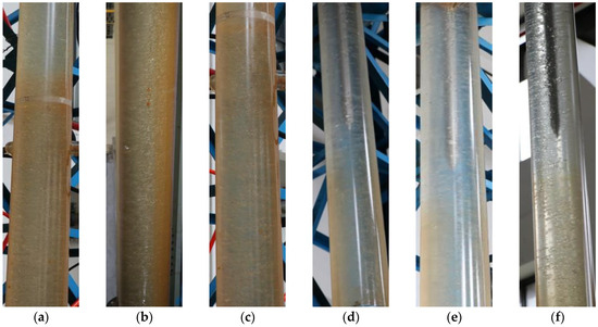
Figure 13.
Flow pattern observation in the simulation test experiment. They should be listed as follows: (a) Q = 40 m3/d, and water cut 60%; (b) Q = 40 m3/d, and water cut 70%; (c) Q = 40 m3/d, and water cut 80%; (d) Q = 30 m3/d, and water cut 60%; (e) Q = 30 m3/d, and water cut 70%; and (f) Q = 30 m3/d, and water cut 75%.

Figure 14.
Response of the capacitive water-cut meter over time.
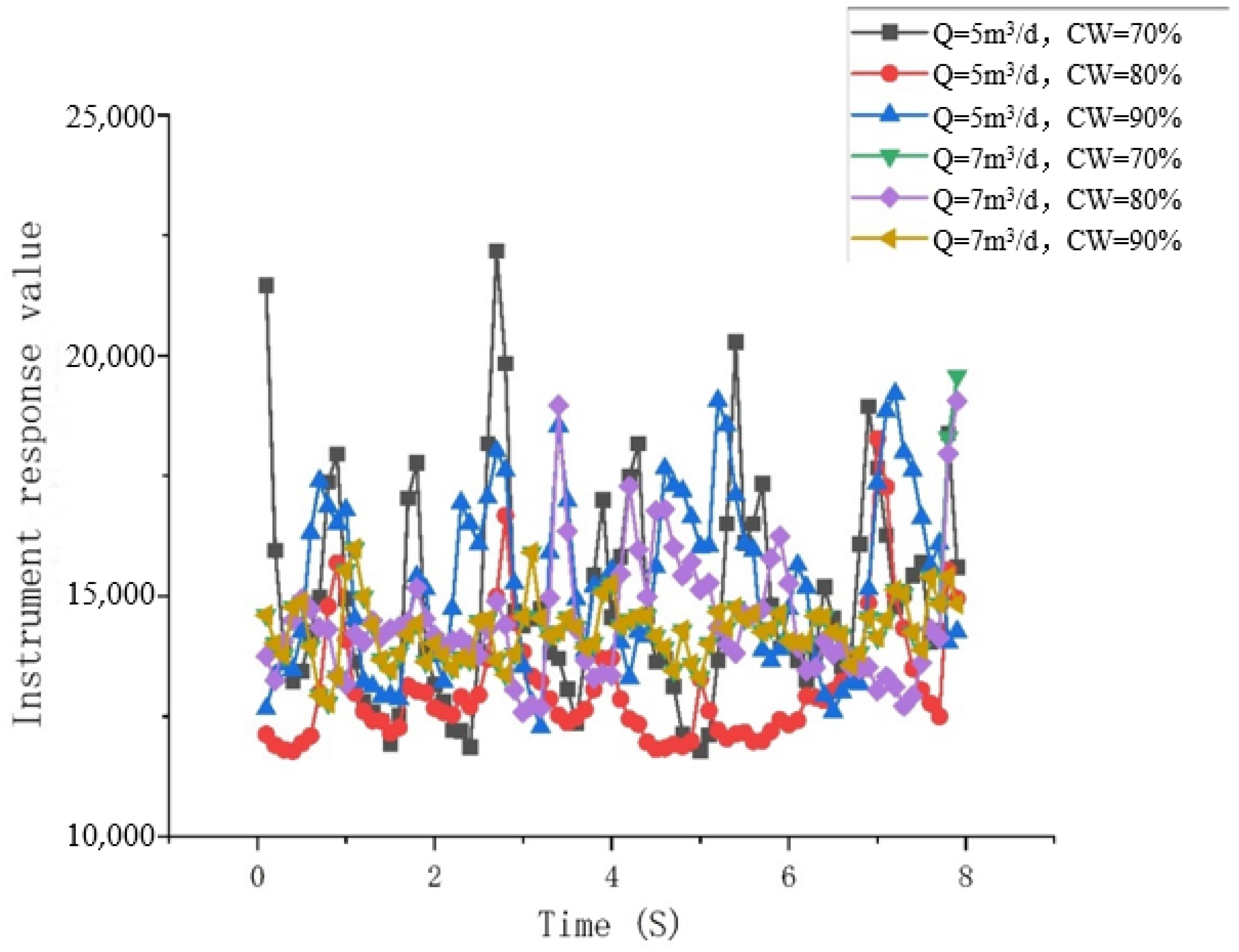
Pulsating Bubble Flow: Water is the continuous phase, and the oil bubbles rise intermittently in a pulsating manner, staying at the center of the pipe, clearly visible. Due to the pulsating upward movement of the oil bubbles, the response value of the capacitive water-cut meter significantly increases when a pulse of oil bubbles reaches it, as shown in Figure 15 and Figure 16.
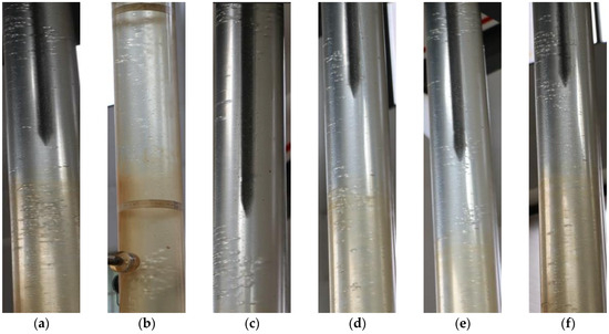
Figure 15.
Observation of flow pattern in the simulation test experiment. They should be listed as follows: (a) Q = 5 m3/d, and water cut 70%; (b) Q = 5 m3/d, and water cut 80%; (c) Q = 5 m3/d, and water cut 90%; (d) Q = 7 m3/d, and water cut 70%; (e) Q = 7 m3/d, and water cut 80%; and (f) Q = 7 m3/d, and water cut 90%.
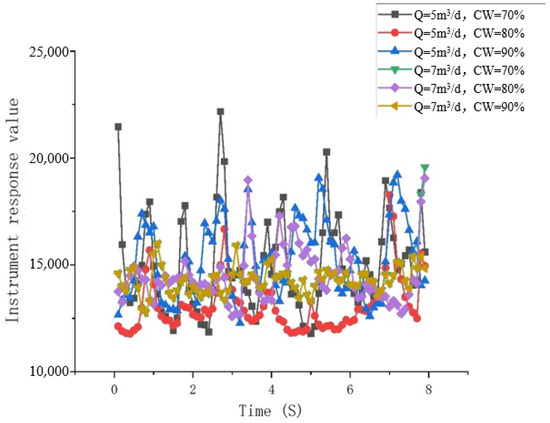
Figure 16.
Response chart of capacitance water-cut meter versus time.
4. Research on Oil–Water Two-Phase Flow Pattern Recognition Based on GA-BP Algorithm
The identification of oil–water two-phase flow patterns is not only the foundation of production profile interpretation but also directly affects the accuracy of production data and the scientific prediction of production well behavior. Different flow patterns lead to different interpretation parameters. Conventional flow pattern identification in production logging generally relies on experimental simulations or numerical simulations. However, both methods are inevitably influenced by subjective factors, making it difficult to achieve objective flow pattern identification. Additionally, due to the constraints of production well conditions, direct measurement methods for flow patterns are often ineffective.
With the development of computers, the wave of artificial intelligence has begun to rise, and neural networks have shown significant advantages in data classification and prediction. Therefore, a neural network algorithm is proposed for the identification of oil–water two-phase flow types. The neural network technology can fully utilize logging data and perform automatic and intelligent flow pattern recognition, avoiding subjective judgment by personnel. This is crucial for improving the accuracy and efficiency of flow type identification.
4.1. BP Neural Network Principle
A BP (backpropagation) neural network is a supervised learning algorithm based on multilayer feedforward neural networks, widely used for tasks such as classification, regression, and feature extraction [37]. Effectiveness in Handling Nonlinear Relationships: The BP neural network excels at modeling complex nonlinear relationships, which is essential for capturing the nonlinear characteristics of the oil–water two-phase flow system. The BP network can learn and approximate these relationships through training, thus improving the prediction accuracy. Flexibility and Customizability: The BP model offers high flexibility in terms of network structure, such as the number of layers and neurons, which can be adjusted and optimized based on the specific requirements of the oil–water two-phase flow problem. This adaptability allows the model to account for the complex dynamic variations in different oil field environments, particularly under specific conditions, like high-water-cut oil wells. Its core idea is to calculate the error and propagate the error backward to adjust the network weights, making the predicted result closer to the true value. The principle of the BP neural network can be divided into the following steps:
Network Structure: The BP neural network consists of an input layer, hidden layer, and output layer. Neurons in each layer are connected by weights. The input layer receives input data, which are processed through the hidden layer, and finally, the output layer generates the predicted result.
Forward Propagation: Input data are passed through the network from the input layer to the hidden layer and then to the output layer. Neurons in each layer receive the output of the previous layer’s neurons, process it through weighted summation and an activation function, and then pass it to the next layer. Activation functions (such as sigmoid, ReLU, etc.) introduce non-linearity, enabling the network to handle complex nonlinear problems.
Loss Function: After calculating the predicted results at the output layer, the difference between the predictions and the actual labels is quantified using a loss function (such as mean squared error, cross-entropy, etc.). For classification tasks, the cross-entropy loss function is commonly used to evaluate the difference between the predicted results and the true labels.
Backpropagation: Through the backpropagation algorithm, the error for each layer is calculated and propagated back through the network. The error is passed layer by layer using the chain rule to compute the gradients for each layer, which indicate how much each weight and bias needs to be adjusted. Then, optimization algorithms like gradient descent or Adam are used to update the weights and biases in order to minimize the loss function.
Training Process: The network undergoes multiple iterations (training epochs), continuously adjusting the parameters (weights and biases) until the loss function converges, and the model’s prediction performance gradually improves.
Classification Prediction: For classification tasks, the trained BP neural network can predict the class of new data by passing it through the forward propagation. The final prediction result is usually the class corresponding to the output layer neuron.
4.2. GA-BP Neural Network Model Construction
The genetic algorithm (GA) is an optimization algorithm that simulates the biological evolution process and belongs to heuristic search methods [38]. It mimics processes in nature such as inheritance, mutation, selection, and crossover to find the optimal or near-optimal solution to a problem.
The genetic algorithm (GA) is widely used in complex optimization problems, especially those with large solution spaces that are difficult to handle by traditional optimization methods. The GA is applicable to various types of problems, including function optimization, combinatorial optimization, and parameter optimization in machine learning models. Its core operations are shown in Table 5.
Table 5.
Core operations of genetic algorithm.
The BP neural network has a powerful fitting ability and adaptability in data classification and prediction. It can handle complex nonlinear relationships and high-dimensional data, automatically learning features, making it suitable for various classification tasks. However, it uses a constant training step size, which leads to a very slow convergence process and often requires additional optimization algorithms. Therefore, due to the limitations of the single algorithm (BP neural network), this section proposes the use of the GA algorithm to optimize the BP neural network algorithm.
The genetic algorithm (GA) applied to optimize the BP neural network algorithm has the following advantages: Avoiding Local Optima: The BP algorithm relies on local information for optimization, which makes it prone to getting stuck in local optima. In contrast, the GA, as a global search algorithm, can effectively avoid this issue. Improving Convergence Speed: The GA accelerates convergence through parallel searching, allowing it to find solutions close to the global optimum in fewer iterations, making it more efficient than BP. Handling Complex Nonlinear Problems: BP assumes that the error function is smooth, which may limit its effectiveness in dealing with complex nonlinear problems. The GA does not rely on this assumption and can address more complicated problems. No Need for Gradient Information: BP requires gradient calculation, which can be complex in certain situations. The GA does not depend on gradients, making it suitable for problems where gradients are either unavailable or computationally expensive. Global Search Capability: BP depends on the initial weights, which can significantly influence the result. The GA, through global search, reduces reliance on the initial solution and is capable of finding the global optimum.
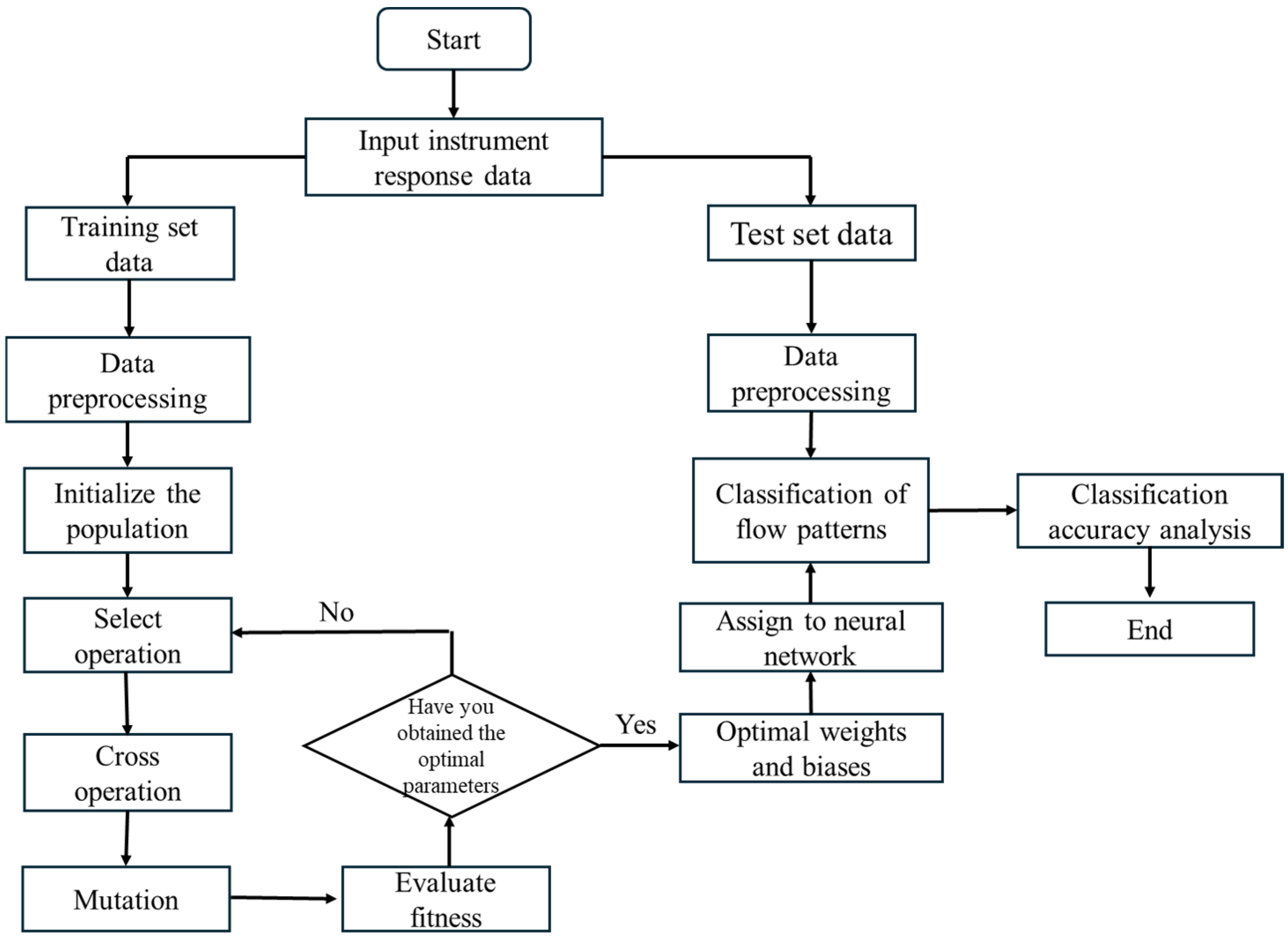
In order to accurately predict phase separation in oil–water two-phase flow, a GA-optimized BP model was constructed. The specific modeling framework is shown in Figure 17, and the detailed implementation steps are as follows:
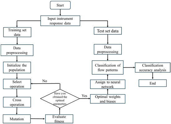
Figure 17.
GA-optimized BP flowchart.
- Randomly select samples and divide them into a training set (100 samples) and a test set (32 samples). The data are divided into input features (2 dimensions) and output labels (6 categories). Data normalization: Normalize the data of the training and test sets to the range [0, 1] to improve the stability of the neural network training.
- Define the neural network structure: Establish a feedforward neural network with 5 nodes in the hidden layer. Set the training parameters: Configure the network’s training parameters, including the maximum number of iterations (1000), target error (1 × 10⁻⁶), and learning rate (0.01).
- Parameter initialization: Set the number of generations for the genetic algorithm to 50, the population size to 5, and the number of parameters to optimize (the total number of network weights and biases). Define the boundary range for the optimization variables as [−1, 1].
- Initialize the population: Generate random candidate solutions, where each individual represents a combination of weights and biases. Optimize the network’s weights and biases through selection, crossover, and mutation operations.
- After the genetic algorithm optimization, decode the best individual to obtain the network’s weights and biases (W1, B1, W2, and B2). Here, W1 represents the weights from the input layer to the hidden layer, W2 represents the weights from the hidden layer to the output layer, B1 is the bias for the hidden layer, and B2 is the bias for the output layer.
- Bring the decoded weights and biases into the neural network to perform simulations on both the training and test sets, obtaining the network’s output. Finally, convert the neural network output into category labels and compare them with the actual category labels.
4.3. Flow Pattern Identification Results
In the oil–water two-phase flow simulation experiment, a total of 132 experimental datasets were collected, including 12 sets of pure oil, 36 sets of emulsion flow, 18 sets of bubbly flow, 40 sets of small bubbly flow, 14 sets of pulsating bubbly flow, and 12 sets of pure water.
The 132 experimental datasets were randomly divided into 100 training set samples and 32 test set samples, with each set containing all the categories of the oil–water two-phase flow patterns.
The flow pattern categories identified using the neural network algorithm were compared with the actual flow pattern categories and plotted, where the x-axis represents the actual flow pattern categories and the y-axis represents the predicted flow pattern categories. The BP neural network flow pattern recognition results and the GA-BP neural network flow pattern recognition results are shown in Figure 18. A comparison table of the real oil–water two-phase flow pattern categories with the BP-predicted categories and GA-BP-predicted categories is presented in Table 6.
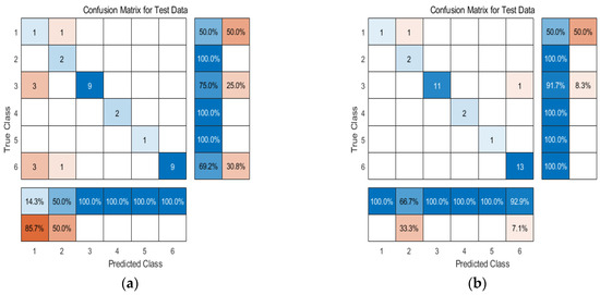
Figure 18.
BP and GA-BP neural network flow pattern prediction results; they should be listed as follows: (a) BP neural network flow pattern prediction results; (b) GA-BP neural network flow pattern prediction results.
Table 6.
Comparison of experimental categories and predicted categories for oil–water two-phase flow patterns.
Based on the above figure and table, a comparison and analysis of the flow pattern prediction results with the actual flow pattern categories shows that the BP neural network flow pattern recognition accuracy is 75%, while the GA-BP neural network flow pattern recognition accuracy is 93.75%. It can be concluded that both neural network algorithms are applicable to oil–water two-phase flow pattern identification, and the GA-BP neural network algorithm achieves a higher accuracy in flow pattern recognition compared to the BP neural network. The GA-BP network algorithm introduces the GA algorithm to optimize the weights and biases of the BP neural network, obtaining the optimal initial weights and biases. This effectively avoids the risk of early convergence to local minima during the BP network training process, thereby improving the accuracy of the oil–water two-phase flow pattern recognition using the neural network algorithm.
5. Production Profile Logging Interpretation Study
For conventional production profile logging interpretation methods, there are mainly two approaches: the experimental plate method and the model method [39]. The experimental plate method is primarily used for interpreting measurements from flow collection instruments in China, while the model method is mainly applied to two-phase flow interpretation. However, many oil fields have entered the later stages of development, where issues such as low-production fluid rates and high water cut are common. In the case of low-production fluids, the turbine flow meter has a threshold for startup speed, meaning the turbine may fail to start or respond unstably. This leads to low response efficiency of the turbine flow meter under low flow conditions. In high-water-cut scenarios, as the water cut increases, the water phase becomes the continuous phase, and the oil phase is distributed in the form of bubbles within the water phase. Due to the high conductivity of water, the oil phase is shielded by the continuous water phase, leading to a low resolution in capacitive water-cut meters [40]. This results in significant errors when using the experimental plate method for interpretation. Artificial intelligence, as an improved computational method, can address the limitations of traditional interpretation methods, enabling efficient and high-quality interpretation of production profile logging.
5.1. RBF Algorithm Principle
In 1988, Broomhead and Lowc introduced the radial basis function (RBF) into neural networks, based on the characteristic of biological neurons having local responses, leading to the development of the RBF network [41]. In 1989, Cybenko demonstrated the ability of the RBF neural network to uniformly approximate nonlinear continuous functions [42].
The radial basis function (RBF) neural network is a feedforward neural network whose core feature is to map input data to a high-dimensional space using a nonlinear activation function. It is commonly used for pattern recognition and regression problems. Due to its advantages in nonlinear mapping, local response, and computational efficiency [43], the RBF network is particularly well suited for complex systems with nonlinear relationships, such as oilfield data. Therefore, the RBF network is chosen as the core model to improve the accuracy and stability of oil–water flow prediction and production profile calculation.
Network Structure: The RBF network typically consists of three layers: Input Layer: This is responsible for receiving the input data, with each input feature corresponding to an input node. Radial Basis Function Layer: Also known as the hidden layer, each neuron in this layer uses a radial basis function as its activation function. The centers and widths of the radial basis functions are usually determined during the network’s training process. Output Layer: This is a linear output layer that linearly combines the outputs of the radial basis function layer to produce the final output.
Radial Basis Function: The radial basis function is the core of the RBF network. Commonly used radial basis functions include Gaussian functions and polynomial functions, among which the Gaussian function is the most common choice. The mathematical form of the Gaussian radial basis function is as follows:
In the equation, the components are defined as follows: is the output of the j-th neuron; x is the input vector; is the center (or mean) of the j-th neuron; and is the width parameter of the j-th neuron.
Training Process: The training process of an RBF network involves determining the centers () and widths () of the radial basis functions, as well as the weights of the output layer. A typical training method includes the following steps: Initialize Centers and Widths: The centers of the radial basis functions are usually selected using clustering algorithms, such as K-means. The widths can either be initialized with a consistent value or determined using cross-validation. Train Output Layer Weights: Using linear regression or other optimization algorithms, the weights of the output layer are adjusted by minimizing the error between the predicted output and the actual output. This is typically performed by solving a system of equations or applying a least-squares optimization approach.
5.2. GHOA-RBF Algorithm Model Construction
The GHOA is a novel swarm intelligence optimization algorithm that combines the advantages of the grey wolf optimization (GWO) algorithm [44] and the falcon optimization algorithm (FOA) [45] to enhance the global search ability and avoid getting trapped in local optima.
The process of optimizing the RBF (radial basis function) neural network using the GHOA (grey wolf and falcon optimization algorithm) mainly includes the following steps, aiming to optimize the hyperparameter of expansion speed in RBF network. By setting the population size to 10, the maximum iteration number to 20, and the search range of the expansion speed between 0.01 and 1000, the GHOA successfully optimized this hyperparameter and improved the regression prediction performance. The GHOA combines the grey wolf optimization (GWO) and falcon optimization (FOA) algorithms, enabling RBF networks to better perform nonlinear modeling.
The GHOA mainly consists of two behavioral mechanisms: 1. Grey Wolf Behavior: This simulates the hunting behavior of a grey wolf pack, using hunting strategies for global search; 2. Falcon Behavior: This simulates the attack strategy of a falcon, providing more precise local search capabilities.
- Initialize RBF Network Parameters: First, the basic parameters of the RBF network are initialized: the input layer accepts the input data (the turbine speed, capacitance water-holding capacity meter response values, and the flow patterns classified by the GA-BP algorithm); the hidden layer is composed of multiple RBF basis functions, each having a center point and a width parameter (σ); and the output layer is used to output the regression results (oil–water flow rate).
- Define Objective Function (Fitness Function): The objective function is typically the mean squared error (MSE), which is used to evaluate the prediction performance of the RBF network. Its expression is as follows:In the equation, is the actual value of the i-th sample; is the output value predicted by the RBF network for the i-th sample; and N is the total number of samples.
- Initialize GHOA Population: In the GHOA, individuals in the population represent the parameter configurations of the RBF network. Each individual contains the following parameters: center points (C): the center points of the hidden layer nodes; width parameter (σ): the width of each radial basis function, controlling its influence range; and weights (W): the connection weights between the hidden layer and the output layer.
- Calculate Fitness Value: For each individual, the current center points, width parameters, and weights are used to train the RBF network and calculate the predicted results. Then, the fitness of each individual based on the objective function (mean squared error) is evaluated:The lower the fitness value, the better the performance of the current individual.
- Update Individual Positions (Optimization Process of GHOA): According to the optimization process of the GHOA, the individuals in the population are updated by simulating the hunting behavior of grey wolves and the attacking behavior of falcons. Grey Wolf Optimization (Global Search): Tracking: grey wolves track the position of their prey and continuously adjust their search area, updating the positions of individuals; encircling: grey wolves search around the position of the prey during the search process, ensuring they can find potential optimal solutions; and attacking: when the grey wolves get close to their prey, they launch a rapid attack to find the optimal solution. Falcon Optimization (Local Search): The falcon optimization part is responsible for fine-tuning the solution found by the grey wolf. The falcon simulates its precise attack on prey, making accurate adjustments to further optimize the current solution. In the GHOA, the falcon optimization helps fine-tune the parameters of each individual, allowing for a more granular adjustment and improving the accuracy of the solution.
- Update Global Optimal Solution: Through the GHOA’s global search (grey wolf optimization) and local fine search (falcon optimization), the global optimal solution is updated. After each update, the new fitness value is calculated, and the individual with the smallest fitness value is recorded as the current optimal solution.
- Determine Termination Condition: Typically, the GHOA will determine whether to stop the iteration based on one of the following conditions: reaching the maximum number of iterations; fitness convergence (i.e., the change in the optimal solution is smaller than a preset threshold). If the termination condition is met, the optimization process ends; otherwise, it returns to step 5 and continues the optimization.
- Extract the Optimal Solution: After GHOA optimization, the optimal center points, width parameters, and weights are obtained. These optimal parameters will be used for the final training of the RBF neural network.
- Train the Final RBF Network: Using the optimal center points, width parameters, and weights obtained through GHOA optimization, the final RBF network is trained and it is used for the regression prediction task.
- Perform Regression Prediction: The trained RBF network is used to perform regression prediction on new data and obtain the output results.
5.3. Example Applications
The feasibility of applying the GHOA-RBF algorithm to the interpretation of production profiles was verified by selecting the dataset obtained from the surface simulation tests as the training set for training.
Input layer: The turbine speed and capacitance response values measured by the combined instruments were selected. At the same time, to verify that the flow regime plays a guiding role in the interpretation of production profiles, the GA-BP neural network algorithm was used to classify the flow patterns based on the experimental dataset obtained from production well test simulations. These classified flow patterns were then applied as input parameters to the GHOA-RBF algorithm.
Output layer: The output layer consists of two units, representing the water flow rate and oil flow rate, respectively.
To further illustrate the optimization effect of the GHOA on the RBF neural network and the guiding role of the flow regime in production profile logging interpretation, a comparison is made between the RBF neural network, the GHOA-RBF algorithm, and the GHOA-RBF algorithm with flow regime input.
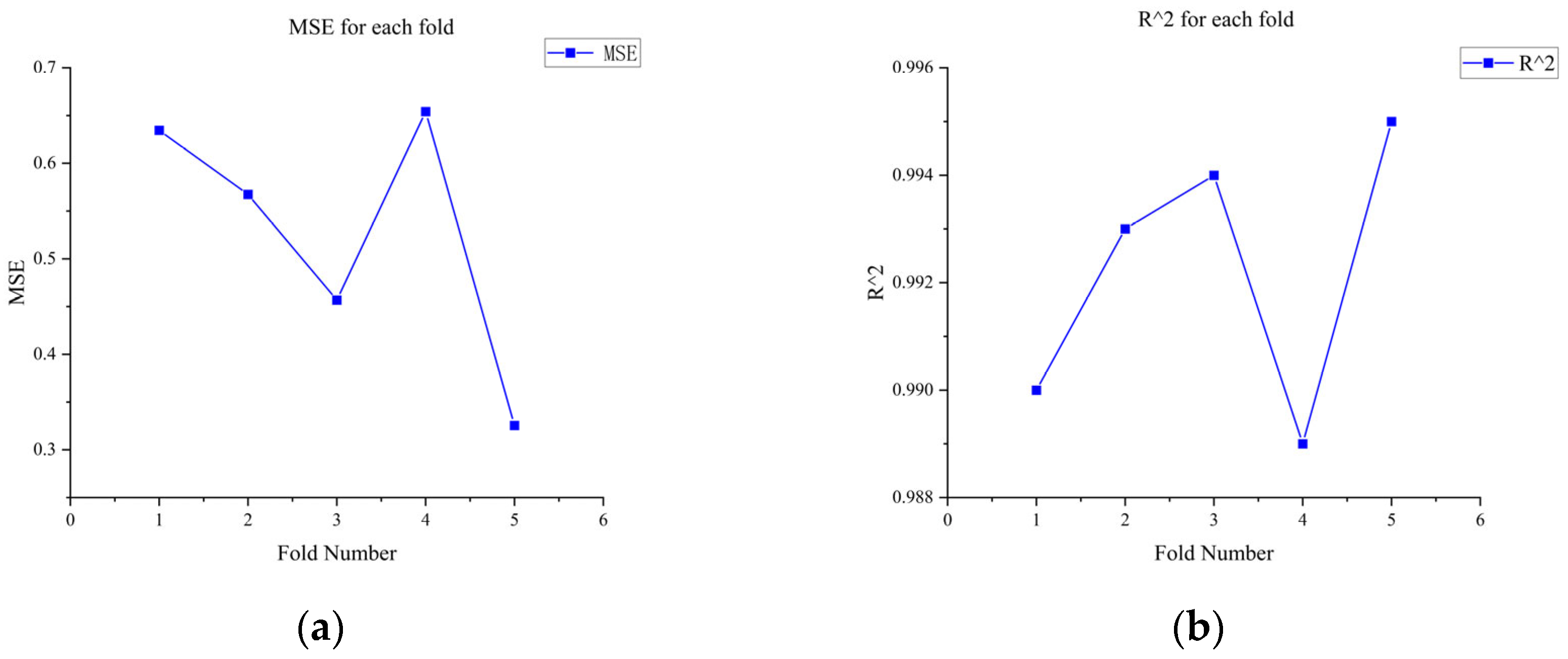
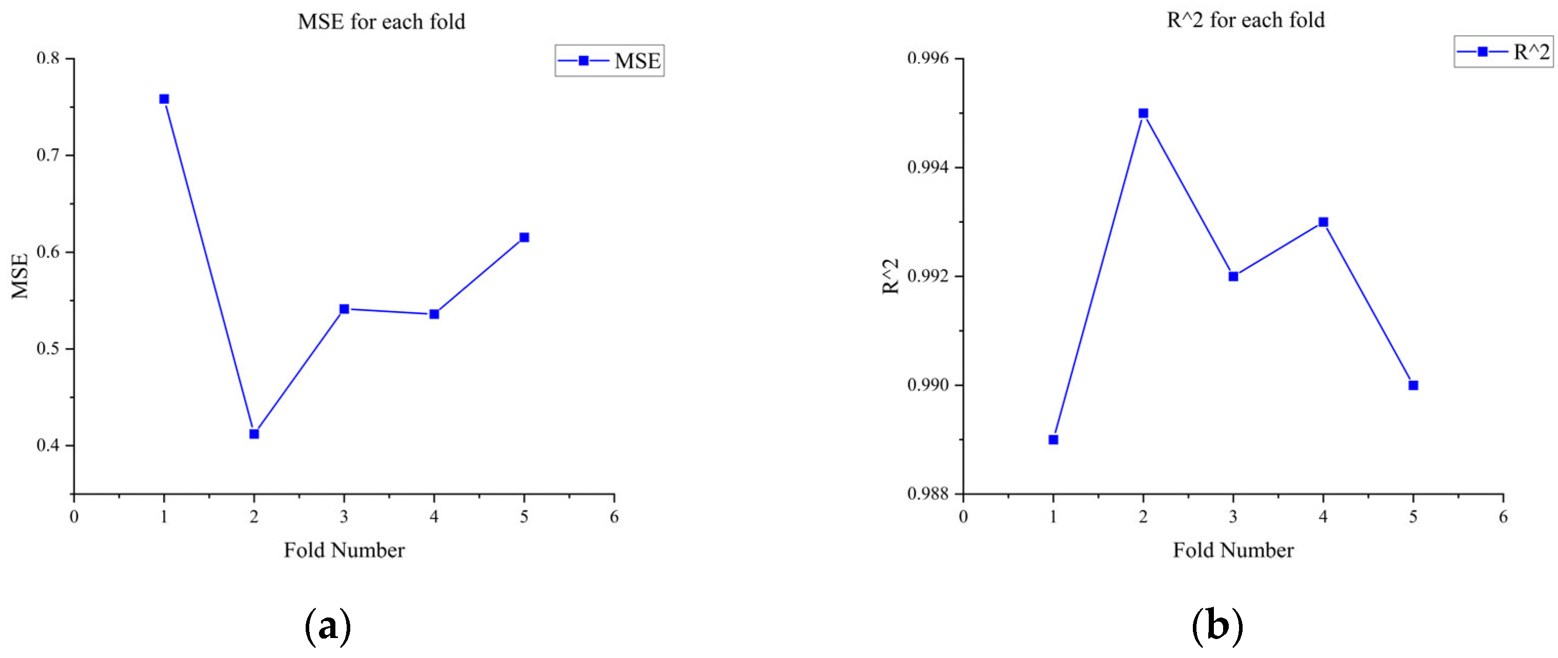
To verify the generalization ability of the proposed GHOA-RBF model and reduce the risk of overfitting, k-fold cross-validation was employed in this study. Specifically, the dataset was evenly divided into k = 5 subsets, and in each iteration, k − 1 subsets were used as the training set, while the remaining subset served as the test set. This process was repeated k times to ensure that each subset was used as the test set for evaluation. In each fold, the grey wolf and hunting falcon optimization algorithm (GHOA) was used to optimize the hyperparameters of the radial basis function (RBF) model, and the model’s predictive performance was then evaluated on the test set. Finally, the average performance metrics for each multiple, such as the mean square error (MSE) and coefficient of determination (R2), were calculated to evaluate the stability and reliability of the model, as shown in Figure 19 and Figure 20. This cross-validation method effectively prevents overfitting of the model to specific data segmentation, providing a more robust performance evaluation.
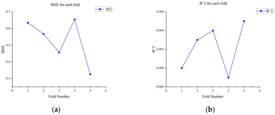
Figure 19.
Cross-validation of MSE and R2 values for each fold of oil flow rate; they should be listed as follows: (a) MSE value for each fold of oil flow prediction; (b) predict the R2 value for each discount of oil flow rate.
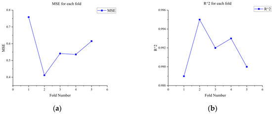
Figure 20.
Cross-validation of MSE and R2 values for each fold of water flow rate; they should be listed as follows: (a) MSE value for each fold of water flow prediction; (b) predict the R2 value for each discount of water flow rate.
To avoid the model “learning the fixed order of the samples”, which could lead to distorted prediction results [46], the 132 data samples obtained from the experiment were randomly shuffled. The shuffled data were then input into the network for training. A total of 112 data samples were used for training, and 20 samples were used for testing, with the training and testing data being consistent across the three methods.
To better assess the predictive performance of the model and evaluate the accuracy of the predicted values, it is necessary to define evaluation metrics for the prediction model. Several evaluation metrics were selected: mean square error (MSE), coefficient of determination (R2), and Residual Prediction Deviation (RPD). The formulas for the evaluation metrics are as follows:
where represents the predicted flow rate of the i-th sample; represents the actual measured flow rate of the i-th sample; and represents the average predicted value of the samples.
Generally, the smaller the MSE, the closer the predicted values are to the true values, indicating better prediction performance. This also suggests that the model has strong generalization ability. A larger R2 and RPD value indicates a higher degree of fit between the predicted and actual values, meaning the model is more accurate.
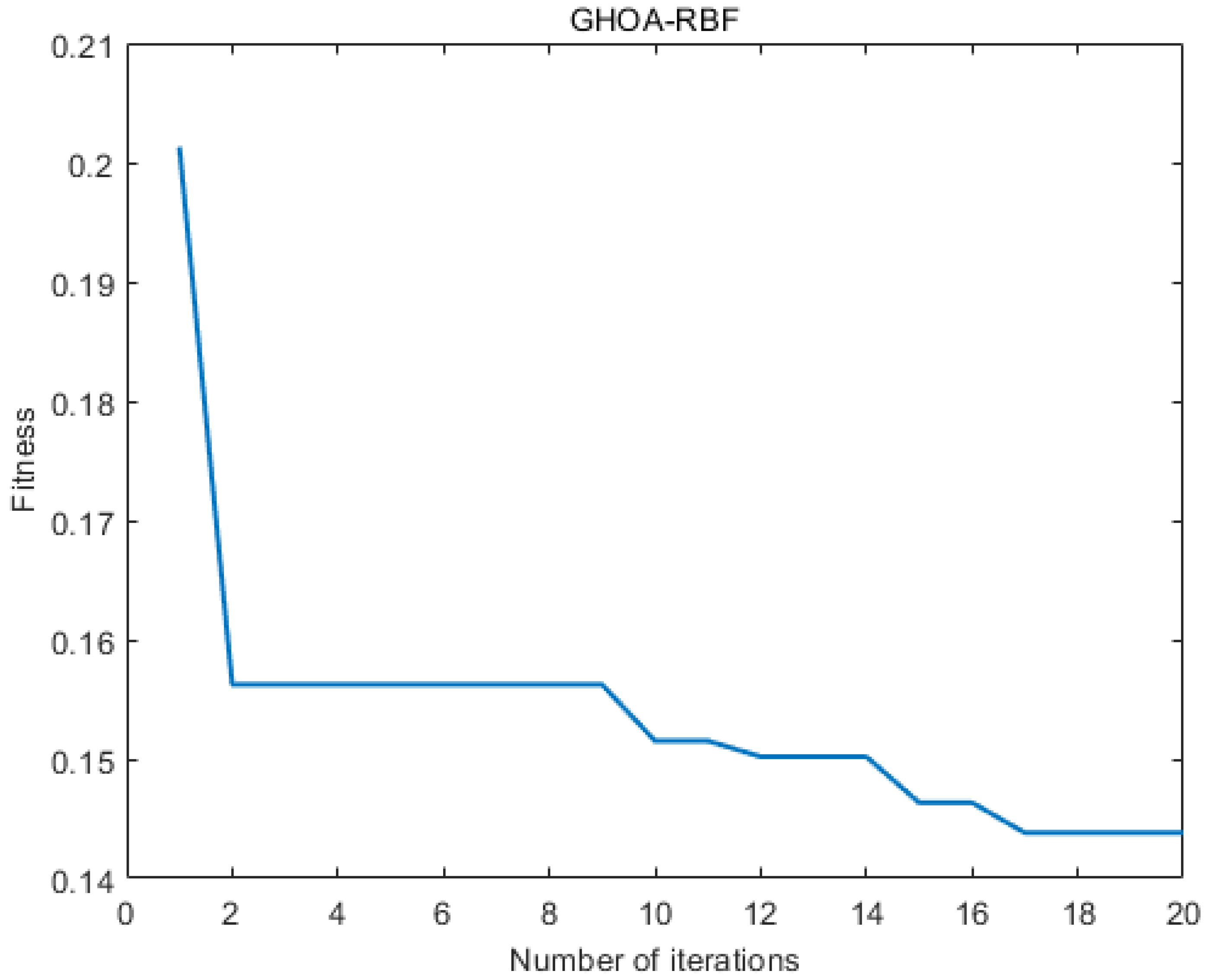
Figure 21 illustrates the variation in fitness over iterations. The fitness reaches near-optimal values by the 20th iteration, and the iteration time is approximately 20 s. The prediction results are shown in Table 7 and Table 8 and Figure 22, Figure 23 and Figure 24. From the tables, it can be seen that the mean squared error (MSE) for oil flow prediction using the GHOA-RBF algorithm is 0.44898, with an R2 of 0.996 and a PRD of 17.3264. For water flow prediction, the MSE is 0.59826, with an R2 of 0.993 and a PRD of 12.5224, indicating that the GHOA-RBF algorithm with flow type classification provides high predictive accuracy. The comparison between the predicted and actual results also shows that, among the three algorithms, the GHOA-RBF algorithm with flow type classification has the highest explanatory accuracy, followed by the GHOA-RBF without flow type classification, and the RBF neural network demonstrates the lowest predictive accuracy.
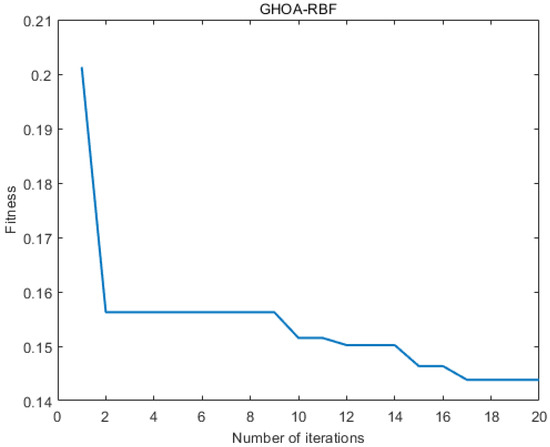
Figure 21.
GHOA-RBF iterative fitness change graph.
Table 7.
Comparison of oil flow model prediction results.
Table 8.
Comparison of water flow model prediction results.

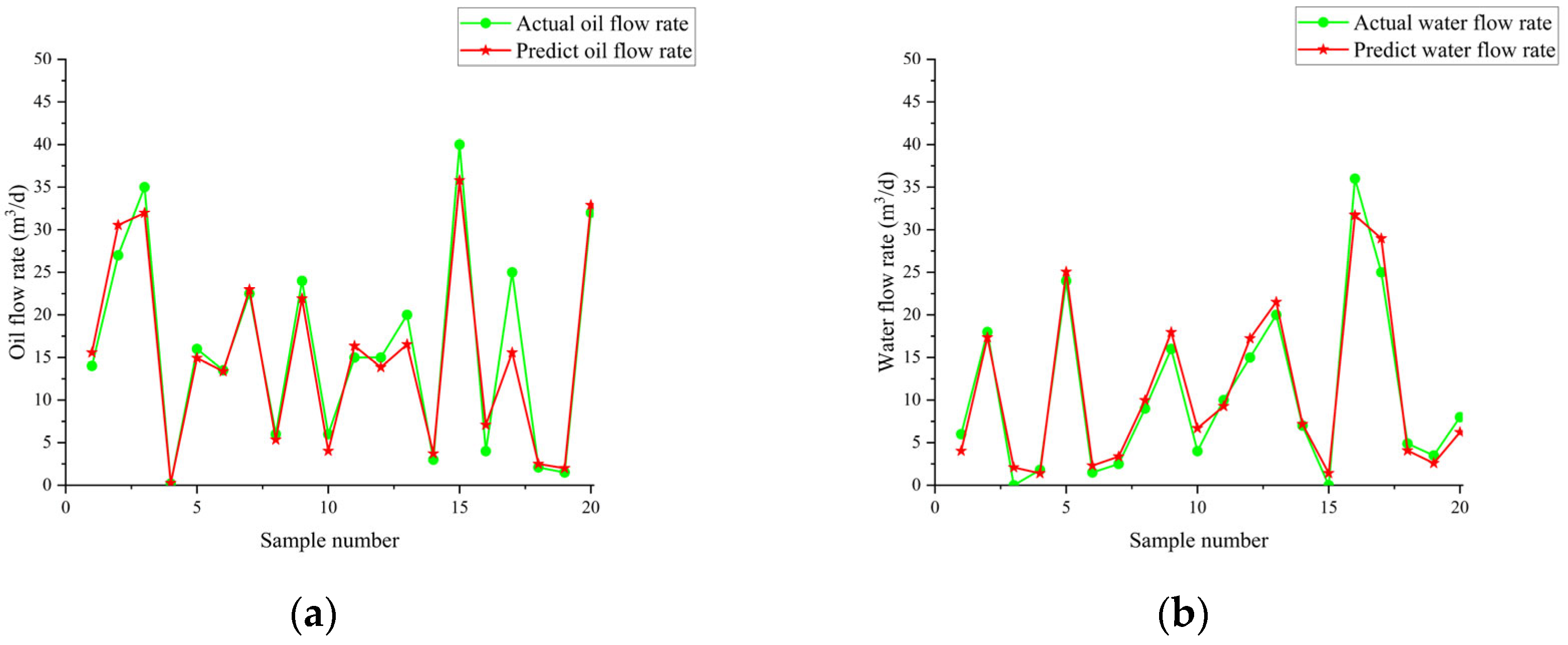
Figure 22.
RBF neural network traffic prediction results; they should be listed as follows: (a) oil flow prediction result; (b) water flow prediction result.
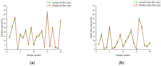
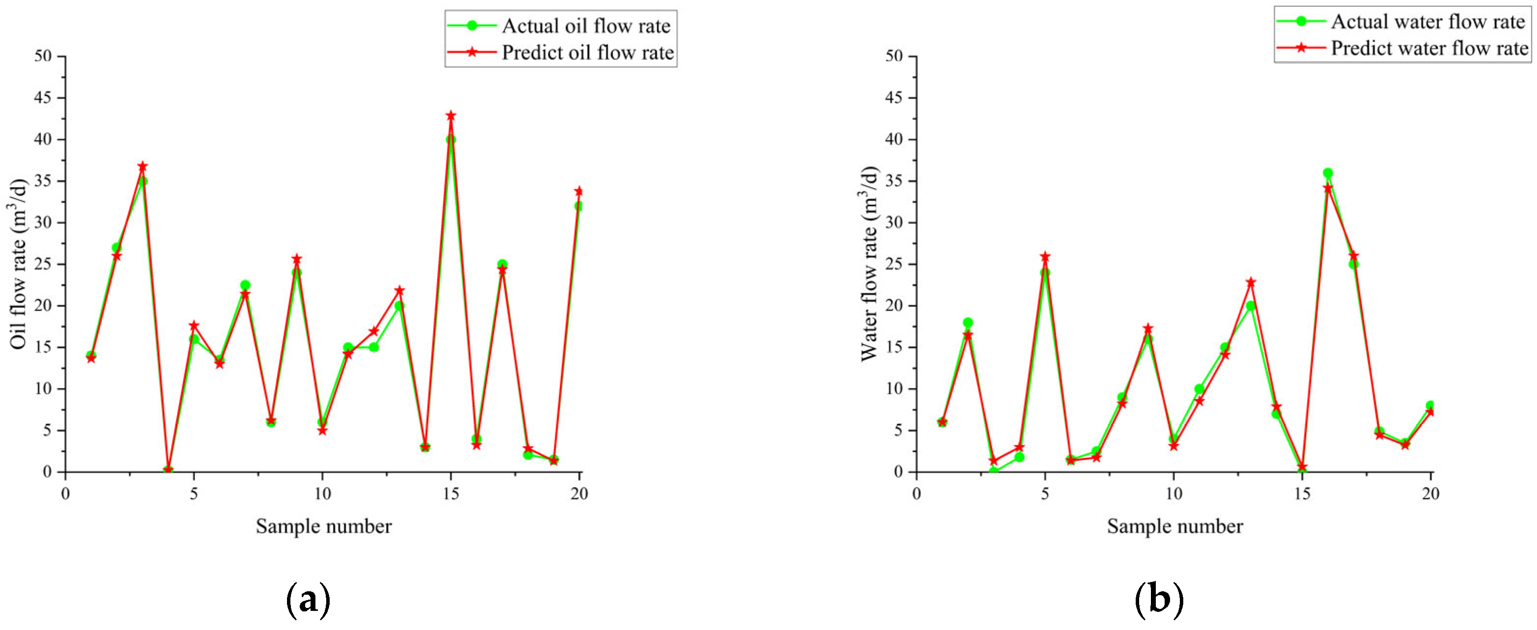
Figure 23.
Flow prediction results of GHOA-RBF algorithm without added flow pattern; they should be listed as follows: (a) oil flow prediction result; (b) water flow prediction result.
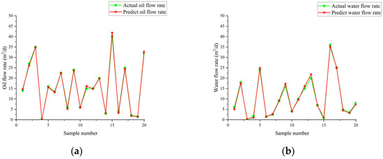
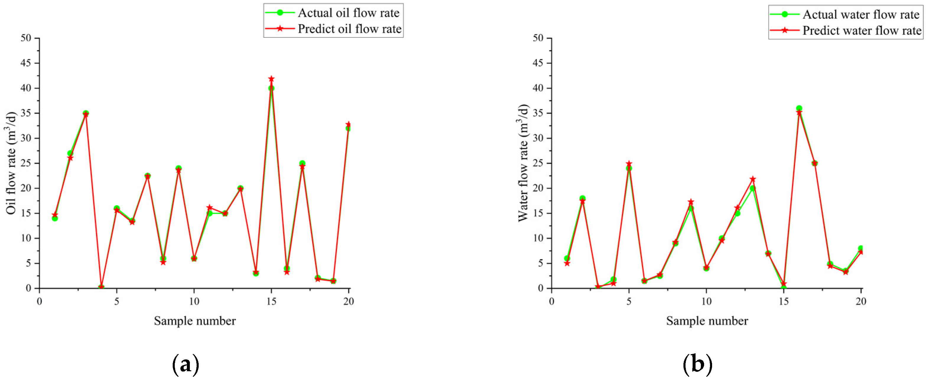
Figure 24.
Flow prediction results of GHOA-RBF algorithm with added flow pattern; they should be listed as follows: (a) oil flow prediction result; (b) water flow prediction result.
6. Conclusions
This study proposes an efficient production profile logging interpretation method based on oil–water two-phase flow numerical simulation, field experiments, and artificial intelligence algorithms. By combining numerical models, experimental data, and a GA-BP neural network optimized GHOA-RBF algorithm, the method significantly improves the accuracy of oil–water two-phase flow pattern recognition and enables precise production profile logging interpretation for high-water-cut oil–water two-phase flow. The experimental results show that the GHOA-RBF algorithm with flow pattern classification demonstrates superior predictive accuracy in oil and water flow rate predictions.
However, the limitations of the model should not be overlooked. Firstly, the training data used for the existing model primarily come from vertical well conditions, and they have not fully considered the adaptability under complex geological conditions (such as unconventional oilfields) or extreme operating conditions. Therefore, the application of the model needs further validation under various conditions and complex oilfield environments. Secondly, although flow pattern classification improves prediction accuracy, there is still room for optimization in computational efficiency when applied to large-scale datasets.
Future research should further expand the model’s adaptability by considering more types of oilfields and operating conditions and improving computational efficiency to ensure that the method can be widely applied in actual production. Overall, this study provides new theoretical support for the production profile logging interpretation of oil–water two-phase flow and has strong practical significance, but further validation and refinement are necessary to address more complex oilfield conditions.
Author Contributions
T.Z.: Methodology, Writing—original draft, Writing—review and editing; H.S.: Methodology, Funding acquisition, Conceptualization; M.L.: Resource. All authors have read and agreed to the published version of the manuscript.
Funding
This work was supported by the National Natural Science Foundation of China (42174155).
Data Availability Statement
The data presented in this study are available on request from the corresponding author. The data are not publicly available due to restrictions of privacy.
Acknowledgments
All the authors would like to thank the reviewers and editors for their thoughtful comments that greatly improved the manuscript.
Conflicts of Interest
Author Hongwei Song is affiliated with the company China National Petroleum Corporation. Author Ming Li is affiliated with the company Qinghai Oilfield Testing Company. The remaining author declares that the research was conducted in the absence of any commercial or financial relationships that could be construed as a potential conflict of interest.
References
- Xue, L.; Liu, P.; Zhang, Y. Status and prospect of improved oil recovery technology of high water cut reservoirs. Water 2023, 15, 1342. [Google Scholar] [CrossRef]
- Wang, N.; Tan, C.; Dong, F. Water holdup measurement of oil-water two-phase flow based on KPLS regression. In Proceedings of the 2015 Chinese Automation Congress (CAC), Wuhan, China, 28–30 July 2015; pp. 1896–1900. [Google Scholar]
- Burrus, B. Determination of Oil and Water Volumes by the Capacitance Method; Society of Petroleum Engineers: Kuala Lumpur, Malaysia, 1966. [Google Scholar]
- Maxit, J.O.; Reittinger, P.W.; Wang, J.; Kostelnicek, R.J. Downhole instrumentation for the measurement of three-phase volume fractions and phase velocities in horizontal wells. J. Energy Resour. Technol. 2000, 122, 56–60. [Google Scholar] [CrossRef]
- Ryan, N.D.; Hayes, D. A new multiphase holdup tool for horizontal wells. In Proceedings of the SPWLA 42nd Annual Logging Symposium, Houston, TX, USA, 17–20 June 2001; pp. 1–5. [Google Scholar]
- Ma, J. Study on the Measurement Method of Water Holding Ratio in Oil-Water Two-Phase Flow Using High-Frequency Sensors. Ph.D. Thesis, Tianjin University, Tianjin, China, 2019. [Google Scholar]
- Guo, H.; Zhang, B. Study on the method of measuring water holding ratio in the wellbore using conductivity method. J. Jianghan Pet. Inst. 1994, 16, 37–41. [Google Scholar]
- Xu, W.; Xu, L.; Cao, Z.; Chen, J.; Liu, X.; Hu, J. Normalized least-square method for water hold-up measurement in stratified oil–water flow. Flow Meas. Instrum. 2012, 27, 71–80. [Google Scholar] [CrossRef]
- Zhong, X.; Jin, Z.; Guo, H.; Li, Q.; Zhang, X. Effect of salinity on the response of radioactive density–water cut meter. J. Jianghan Pet. Inst. 1996, 01, 55–58. [Google Scholar]
- Yang, Q. Laboratory experimental study of radioactive three-phase flow logging instrument. Pet. Instrum. 2012, 26, 38+9. [Google Scholar]
- Hatton, G.J.; Helms, D.A.; Marrelli, J.D.; Durrett, M.G. A new microwave-based water-cut monitor technology. In Proceedings of the Offshore Technology Conference, Houston, TX, USA, 7–10 May 1990. [Google Scholar]
- Liu, X.; Yuan, Z.; Liu, Q.; Zhang, X.; Zhuang, H. Establishment of a theoretical model for high water cut measurement using ultra-short wave water cut meter. J. Metrol. 1995, 16. [Google Scholar]
- Hao, X.-Y.; Li, X.-B.; Zhang, H.-N.; Zhang, W.-H.; Li, F.-C. Review on multi-parameter simultaneous measurement techniques for multiphase flow—Part B: Basic physical parameters and phase characteristics. Measurement 2023, 220, 113397. [Google Scholar] [CrossRef]
- Govier, G.W.; Sullivan, G.A.; Wood, R.K. The upward vertical flow of oil-water mixtures. Can. J. Chem. Eng. 1961, 39, 67–75. [Google Scholar] [CrossRef]
- Zavareh, F.; Hill, A.D.; Podio, A. Flow regimes in vertical and inclined oil/water flow in pipes. In Proceedings of the SPE Annual Technical Conference and Exhibition, Houston, TX, USA, 2–5 October 1988; Society of Petroleum Engineers: Kuala Lumpur, Malaysia, 1988. [Google Scholar]
- Flores, J.G.; Chen, X.T.; Sarica, C.; Brill, J.P. Characterization of oil-water flow patterns in vertical and deviated wells. In Proceedings of the SPE Annual Technical Conference and Exhibition, San Antonio, TX, USA, 5–8 October 1997. [Google Scholar]
- Zhong, X.; Huang, Z.; Lv, P.; Xie, R.; Li, Q. Study on flow pattern identification of oil-water two-phase flow in a 125mm vertical round pipe. J. Pet. 2001, 22, 89–94. [Google Scholar]
- Jin, N.D.; Nie, X.B.; Ren, Y.Y.; Liu, X.B. Characterization of oil-water two-phase flow patterns in a vertical upward pipe. Chem. Eng. J. 2001, 52, 907–915. [Google Scholar]
- Li, Y.; Yu, L.; Kong, L. Oil-water two-phase flow pattern recognition based on multi-feature LS-SVM. J. Yanshan Univ. 2008, 32, 258–262. [Google Scholar]
- Ma, K.; Guo, L.; Jiang, R.; Zhang, X.; Wu, G. Numerical study of oil-water dispersed flow in a vertical pipe. J. Eng. Thermophys. 2011, 32, 1513–1515. [Google Scholar]
- Yao, Q. Experimental Study on the Flow Behavior of Two-Phase Flow and Sensor Response in Small-Diameter Vertical Pipes. Ph.D. Thesis, Northeast Petroleum University, Daqing, China, 2012. [Google Scholar]
- Yin, H. Study on the Prediction of Oil Bubble Flow Coalescence and Flow Pattern Recognition Method in Vertical Pipelines. Ph.D. Thesis, Tianjin University of Science and Technology, Tianjin, China, 2020. [Google Scholar]
- Chen, Q.; Yu, H.; Wei, Y. Implementation of the mixer circuit in the electromagnetic wave phase shift detection method for water cut measurement. J. Pet. Nat. Gas 2012, 34, 221–224. [Google Scholar]
- Jiang, J. Study on the slip velocity of gas-liquid flow in vertical casings. Geophys. Logging 1991, 15, 286–291. [Google Scholar]
- Wang, Z.; Wu, X.; Zhang, S. Sliding model for production logging interpretation of two-phase flow in vertical wells. Pet. Geophys. Prospect. 2003, 42, 276–278. [Google Scholar]
- Chen, K.; Li, M.; Yang, G.; Guo, C.; Wang, H.; Chen, Y. Interpretation method of liquid production profile logging using the Φ23 flow collection-type water-cut combination logging tool. Logging Technol. 2018, 42, 205–209. [Google Scholar]
- Zhang, S.; Guo, H.; Shi, X. Application of simulated annealing PSO optimization algorithm in oil-water two-phase flow production profile interpretation. Logging Technol. 2010, 34, 289–292. [Google Scholar]
- Zhou, Z. Study on the Interpretation Method of Well Testing and Logging Data Based on Deep Learning. Ph.D. Thesis, Hefei University of Technology, Hefei, China, 2021. [Google Scholar]
- Frooqnia, A.; A-Pour, R.; Torres-Verdín, C.; Sepehrnoori, K. Numerical simulation and interpretation of production logging measurements using a new coupled wellbore-reservoir model. In Proceedings of the SPWLA 52nd Annual Logging Symposium, Colorado Springs, CO, USA, 14–18 May 2011. [Google Scholar]
- Aliyeva, T.; Czuprat, O.; Byrski, P. CFD modelling of multiphase flow in horizontal pipe annulus: Effect of sweeping pills on drill cuttings removal. In Proceedings of the SPE Annual Technical Conference and Exhibition, New Orleans, LA, USA, 23–25 September 2024. [Google Scholar]
- Marrah, A.; Rahman, M.A. Erosion rate in a complex pipeline using CFD. In Proceedings of the Gas & Oil Technology Showcase and Conference, Dubai, United Arab Emirates, 13–15 March 2023. [Google Scholar]
- Wheeler, M.P.; Ryan, P.; Cimolin, F.; Gunderson, A.; Scherer, J. Using VOF slip velocity to improve productivity of planing hull CFD simulations. In Proceedings of the SNAME International Conference on Fast Sea Transportation, Providence, RI, USA, 26–27 October 2021. [Google Scholar]
- Olsen, J.J.; Hemmingsen, C.S.; Bergmann, L.; Nielsen, K.K.; Glimberg, S.L.; Walther, J.H. Characterization and erosion modeling of a nozzle-based inflow-control device. SPE Drill. Compl. 2017, 32, 224–233. [Google Scholar] [CrossRef]
- Song, H.; Guo, H.; Guo, S.; Shi, H. Measurement method for phase flow rates of horizontal well oil/water two-phase stratified flow. Pet. Explor. Dev. 2020, 47, 573–582. [Google Scholar] [CrossRef]
- Cmelik, H.R.M.; Sarabian, R.A. Quantitative analysis of production logs in two-phase liquid-gas systems. In Proceedings of the SPE Production Technology Symposium, Lubbock, TX, USA, 5–6 November 1979. [Google Scholar]
- Schlumberger. Production Logging Interpretation, 3rd ed.; Schlumberger: Houston, TX, USA, 1973. [Google Scholar]
- Rumelhart, D.; Hinton, G.; Williams, R. Learning representations by back-propagating errors. Nature 1986, 323, 533–536. [Google Scholar] [CrossRef]
- Holland, J.H. Adaptation in Natural and Artificial Systems; University of Michigan Press: Ann Arbor, MI, USA, 1975. [Google Scholar]
- Guo, H.; Song, H.; Liu, J. Principles of Production Logging and Data Interpretation; Petroleum Industry Press: Beijing, China, 2021. [Google Scholar]
- Wang, M.; Song, H.; Li, M.; Wu, C. Prediction of split-phase flow of low-velocity oil-water two-phase flow based on PLS-SVR algorithm. J. Pet. Sci. Eng. 2022, 212, 110257. [Google Scholar] [CrossRef]
- Broomhead, D.S.; Lowe, D. Multivariable functional interpolation and adaptive networks. Complex Syst. 1988, 2, 321–355. [Google Scholar]
- Cybenko, G. Approximation by superpositions of a sigmoidal function. Math. Control Signals Syst. 1989, 2, 303–314. [Google Scholar] [CrossRef]
- Wang, A. Research on production logging data interpretation method based on fuzzy neural network. Master’s Thesis, Daqing Petroleum Institute, Daqing, China, 2007. [Google Scholar]
- Mirjalili, S.; Mirjalili, S.M.; Lewis, A. Grey wolf optimizer. Adv. Eng. Softw. 2014, 69, 46–61. [Google Scholar] [CrossRef]
- de Vasconcelos Segundo, E.H.; Mariani, V.C.; dos Santos Coelho, L. Design of heat exchangers using Falcon optimization algorithm. Appl. Therm. Eng. 2019, 156, 119–144. [Google Scholar] [CrossRef]
- Sammut, C.; Webb, G.I. Encyclopedia of Machine Learning and Data Mining; Springer: Berlin/Heidelberg, Germany, 2017. [Google Scholar]


Disclaimer/Publisher’s Note: The statements, opinions and data contained in all publications are solely those of the individual author(s) and contributor(s) and not of MDPI and/or the editor(s). MDPI and/or the editor(s) disclaim responsibility for any injury to people or property resulting from any ideas, methods, instructions or products referred to in the content. |
© 2025 by the authors. Licensee MDPI, Basel, Switzerland. This article is an open access article distributed under the terms and conditions of the Creative Commons Attribution (CC BY) license (https://creativecommons.org/licenses/by/4.0/).