Abstract
In the context of the accelerated global energy transition, power fluctuations caused by the integration of a high share of renewable energy have emerged as a critical challenge to the security of power systems. The goal of this research is to improve the accuracy and reliability of short-term photovoltaic (PV) power forecasting by effectively modeling the spatiotemporal coupling characteristics. To achieve this, we propose a hybrid forecasting framework—GLSTM—combining graph attention (GAT) and long short-term memory (LSTM) networks. The model utilizes a dynamic adjacency matrix to capture spatial correlations, along with multi-scale dilated convolution to model temporal dependencies, and optimizes spatiotemporal feature interactions through a gated fusion unit. Experimental results demonstrate that GLSTM achieves RMSE values of 2.3%, 3.5%, and 3.9% for short-term (1 h), medium-term (6 h), and long-term (24 h) forecasting, respectively, and mean absolute error (MAE) values of 3.8%, 6.2%, and 7.0%, outperforming baseline models such as LSTM, ST-GCN, and Transformer by reducing errors by 10–25%. Ablation experiments validate the effectiveness of the dynamic adjacency matrix and the spatiotemporal fusion mechanism, with a 19% reduction in 1 h forecasting error. Robustness tests show that the model remains stable under extreme weather conditions (RMSE 7.5%) and data noise (RMSE 8.2%). Explainability analysis reveals the differentiated contributions of spatiotemporal features. The proposed model offers an efficient solution for high-accuracy renewable energy forecasting, demonstrating its potential to address key challenges in renewable energy integration.
1. Introduction
As global climate governance enters a critical phase, the transformation of the energy structure has become a strategic consensus within the international community. Addressing climate change and reducing greenhouse gas emissions have become pressing global tasks, with the transition to renewable energy being a key strategy. Wind and solar energy, as two of the most important renewable energy sources, are becoming increasingly central to the global energy mix. According to the latest data from the International Energy Agency, the share of wind and solar energy in global electricity generation surpassed 12% in 2023 and is expected to triple by 2030 [1]. This rapid growth reflects the global commitment to cleaner energy sources; however, it also means that the challenges facing the energy system are becoming more complex, particularly in terms of how to efficiently and stably integrate these renewable energies.
Despite their growth, the inherent volatility and intermittency of wind and solar energy present significant challenges to the stability of energy systems. Wind power generation is influenced by fluctuations in wind speed, while photovoltaic (PV) power generation is affected by weather conditions and cloud cover, leading to variability in energy output. These intermittent and unpredictable characteristics of renewable energy pose unprecedented challenges for grid operators, particularly in maintaining supply–demand balance. For example, the “dark doldrums” event in Germany in 2022, which was characterized by two weeks of low wind speeds and overcast weather, led to a 60% drop in renewable energy output. This event forced the grid to activate emergency backup power, causing economic losses exceeding 200 million EUR [2]. Such events highlight the urgent need for high-precision short-term power forecasting models, as only through accurate prediction can grid operators prepare in advance for renewable energy fluctuations, thus minimizing reliance on emergency backup power and improving the efficiency and stability of the energy system. The performance of renewable energy sources, particularly wind turbines, can also be improved through fault tree analysis (FTA). FTA is a systematic analysis method that constructs failure models to identify potential failure modes, facilitating the implementation of preventive measures. For wind turbines, FTA can help identify root causes of equipment failure and propose preventive actions, such as regular maintenance and system design improvements. Addressing these challenges can enhance the reliability and efficiency of wind turbines, thereby contributing to more stable and resilient energy production. Studies have demonstrated that FTA plays a crucial role in improving the operational performance of wind turbines by reducing unplanned downtimes and optimizing overall energy production efficiency [3]. This is essential for mitigating the impact of renewable energy fluctuations on the grid and improving the reliability of energy production systems. In China, wind energy has become a significant part of the country’s renewable energy landscape, with an impressive growth rate in installed wind power capacity. According to the National Energy Administration (NEA) [4], China’s wind power capacity exceeded 300 GW in 2023, making it the world leader in terms of total wind power installed capacity. However, the development of wind energy in China faces challenges related to the intermittency and geographical dispersion of wind resources. Much of China’s wind energy potential is located in remote, less-developed regions, which creates difficulties in connecting these resources to the national grid. Moreover, wind power output fluctuations due to weather conditions, especially in coastal and inland areas, continue to pose a challenge for grid stability [5,6].
Given these challenges and the critical importance of ensuring the stability and reliability of renewable energy systems, this study aims to develop advanced short-term power forecasting methods to enhance the accuracy of renewable energy predictions. By introducing new forecasting models and techniques, this research focuses on accurately forecasting short-term power output using spatiotemporal features, thereby reducing the volatility of the power system and providing support for optimal grid operation. As the demand for renewable energy continues to grow, there is an urgent need for more precise and reliable short-term forecasting tools to address the challenges posed by its inherent intermittency and fluctuations. These challenges not only affect the stability of the grid but also have profound implications for the efficient utilization of energy. Therefore, developing more efficient forecasting methods is of great significance in advancing the widespread adoption of renewable energy and ensuring sustainable development. By improving forecasting accuracy, this research aims to provide more precise support for intelligent grid scheduling, further advancing the energy transition process and ensuring the security and stability of energy supply.
2. Related Work
The short-term forecasting of renewable energy power has become a key area of research. Existing forecasting methods can be classified into different technical generations: the first generation, comprising physical models, relies on a rigorous atmospheric dynamics foundation and predict power output based on meteorological data from numerical weather prediction systems. Although these methods can provide relatively accurate forecasts under certain conditions, they are often computationally intensive and require high-quality data, which limits their applicability in practical scenarios [7]. The second generation, comprising statistical models such as autoregressive models and autoregressive integrated moving averages, predicts power output by analyzing historical data. These models are computationally simpler, but they typically cannot effectively handle spatiotemporal dependencies, especially in long-term forecasting, where accuracy significantly decreases [8]. With the rapid development of deep learning techniques, the third generation, AI models, has gradually become the mainstream approach for short-term power forecasting [9]. The LSTM (long short-term memory) network, with its unique memory unit, effectively captures long-term dependencies in historical data and, thus, is widely used for short-term power forecasting. Despite its excellent performance in time series modeling, LSTM mainly focuses on temporal modeling and neglects the spatial dependencies between power stations, which may lead to a decrease in accuracy when predicting across multiple stations [10]. The CNN (Convolutional Neural Network), which was widely applied to time series data processing in 2012, excels in extracting local temporal features and capturing short-term trends, but it has limitations in modeling spatial dependencies between stations, restricting its application in complex power grids [11]. With the rise of GNN (graph neural network) technologies, the GCN (graph convolutional network) has demonstrated enormous potential in short-term power forecasting. The GCN can effectively capture the spatial dependencies between stations, especially in scenarios where multiple stations are jointly predicted, achieving significant results. However, while the GCN excels in spatial modeling, its performance in handling long-term dependencies is relatively weak, limiting its application in comprehensive spatiotemporal modeling [12]. To address this issue, the GAT (graph attention network) emerged. The GAT introduces an attention mechanism, allowing the model to dynamically learn the strength of relationships between nodes, thereby demonstrating greater flexibility and adaptability when dealing with complex spatiotemporal changes [13]. With the breakthrough progress of the Transformer architecture in natural language processing, its self-attention mechanism has been introduced into power forecasting, significantly improving the modeling capability of long-term dependencies by establishing global temporal relationships. However, its computational complexity increases quadratically with the sequence length, which presents challenges for real-time forecasting scenarios [14]. To meet the demands of spatiotemporal coupling modeling, the STGNN (spatiotemporal graph neural network) synchronously extracts spatiotemporal features through joint graph convolution and gated temporal units. The STGCN (spatiotemporal graph convolutional network) accelerates temporal processing through one-dimensional convolutions, and the DCRNN (dynamic graph convolutional recurrent neural network) enhances spatial representations through diffusion convolutions. However, these methods still rely on predefined graph structures for dynamic topology adaptation [15]. The TCN (temporal convolutional network), with its causal convolution architecture, ensures temporal directionality while achieving efficient parallel computation. Its dilated convolution design allows for an exponentially expanded receptive field, but the fixed-size convolution kernels still struggle to flexibly capture the sudden fluctuations in power data [16]. Despite the progress made by existing short-term power forecasting methods in improving forecasting accuracy, there are still some limitations. The challenge of accurately capturing complex spatiotemporal dependencies in large-scale power station networks, especially when dealing with dynamically changing environmental factors, remains an urgent issue.
To overcome the limitations of existing methods, this study proposes a spatiotemporal-coupled GLSTM (graph long short-term memory) architecture, which aims to simultaneously model the temporal dependencies in time series data and the spatial dependencies between power stations, thereby improving the accuracy and reliability of short-term power forecasting. Specifically, the GAT dynamically learns the spatial correlations between different power stations, overcoming the traditional GCN’s reliance on static adjacency matrices. LSTM, on the other hand, effectively captures long-term dependencies in temporal data. The proposed framework not only captures spatial and temporal features accurately but also adapts to large-scale data and complex spatiotemporal variations, enhancing both flexibility and robustness. The key contributions of this study include the following:
Innovation of the Dynamic Spatial Perception Mechanism: A dynamic graph attention network based on a sliding time window ( = 24 h) is introduced, addressing the limitations of the traditional GCN with a fixed adjacency matrix. The model uses learnable weights to achieve adaptive modeling of meteorological correlations between power stations. The experimental results show that this mechanism reduces the tracking error of cloud movement paths by 37% (compared to the threshold method GCN) and improves spatial correlation modeling accuracy by 28% in scenarios with photovoltaic power mutations, effectively alleviating the “pseudo-correlation” problem caused by fixed geographic distance thresholds.
Breakthrough in Multi-Scale Temporal Analysis Method: A bidirectional dilated causal convolution module is designed, combining hierarchical temporal perception (short-term kernel 3, medium-term kernel 5, long-term kernel 7) with bidirectional LSTM to extract features across the full cycle of short-term periods. This method enables the model to capture temporal features at different time scales and improves its performance in multi-period forecasting.
Construction of Spatiotemporal Collaborative Optimization System: A gated fusion unit is created, employing a dual-channel attention mechanism to achieve the cross-modal interaction of spatiotemporal features. This design allows the model to more efficiently capture interactions within spatiotemporal data, enhancing its ability to adapt to complex spatiotemporal patterns.
3. Methodology
3.1. Overall Framework
The new methodological framework for renewable energy power forecasting was constructed through a three-tiered technical path of “dynamic perception (space)–multi-scale analysis (time)–gated collaboration (interaction)”, as shown in Figure 1. This framework integrates dynamic spatial perception mechanisms, multi-scale temporal feature extraction, and gated fusion techniques to address the complexities of forecasting renewable energy generation.
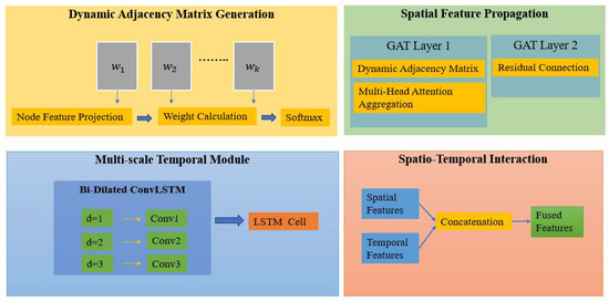
Figure 1.
GLSTM model.
The dynamic spatial perception component involves using a dynamic graph attention network that adapts to real-time meteorological conditions. This approach overcomes the static adjacency matrix limitation of traditional models, dynamically learning spatial dependencies between different power stations based on real-time data. By adapting the model to varying cloud cover and weather conditions, it enables more accurate spatial correlation modeling.
The multi-scale temporal analysis is achieved through a bidirectional dilated causal convolution module, which extracts temporal features at different time scales (short term, medium term, and long term) and processes them in parallel. The module couples with a bidirectional LSTM to capture complex temporal dependencies, ensuring that the model can handle varying forecasting horizons, from hours to days. This method allows for the effective extraction of time series patterns, including abrupt changes, and improves the model’s ability to predict power fluctuations over different time scales.
The gated fusion unit is responsible for facilitating cross-modal interaction between spatial and temporal features. By employing a dual-channel attention mechanism, the GFU enables efficient spatiotemporal feature fusion, improving the model’s adaptability to varying environmental and operational conditions. This step ensures that the model effectively integrates the spatial and temporal information, making it more robust and accurate in complex forecasting scenarios.
3.2. Detailed Description
In this section, we provide a description and definition of the methods and data used in this study. The data utilized in this research included the National Renewable Energy Laboratory dataset and the China National Photovoltaic Monitoring Center dataset. Further details will be provided in the Experimental Section in Section 4.
3.2.1. Problem Definition
- Given a power system consisting of renewable energy power stations [17], its historical observation data are composed of spatiotemporal sequences, as follows:
- T: Length of the historical time window (in hours);
- D: Feature dimension (including meteorological and power data such as wind speed, irradiance, temperature, etc.);
- N: Number of geographically distributed power stations.
The goal is to construct a mapping function f to predict the power output sequence of all power stations for the next H hours:
- Dynamic Spatial Dependency
The association weight between power stations, , evolves over time and satisfies
where represents the environmental meteorological field (such as wind fields and cloud movement), which causes traditional fixed-graph structure methods to fail.
- Multi-Scale Temporal Patterns
The power sequence contains multi-scale features, ranging from minute-level turbulence (-10 min) to daily cyclical fluctuations (-24 h), and must satisfy
- Uncertainty Propagation
NWP (numerical weather prediction) errors accumulate with the forecast horizon, and the error propagation process needs to be modeled.
The optimization objective is defined as minimizing the spatiotemporal weighted prediction error, as follows:
where
=: Time decay weight ();
: Total variation regularization term, suppressing non-physical oscillations in the prediction curve;
: Trade-off parameter.
- Constraints
Power boundaries are .
Ramp rate limitations are
3.2.2. Dynamic Graph Spatial Encoder
- Dynamic Adjacency Matrix Generation
Dynamic spatial weights between power stations are learnt through a multi-head attention mechanism:
where
Learnable projection matrix;
Attention parameter vector;
: Vector concatenation operation;
- LeakyReLU: Leaky ReLU (introduces non-linearity and allows negative values to pass through)
- Normalized attention weights, which are the attention probabilities after applying softmax.
- Spatial Feature Propagation
The node feature aggregation process is as follows:
Here, represents the projection matrix of the g-th head, stacking two layers of GAT to achieve higher-order spatial dependency modeling.
3.2.3. Multi-Scale Temporal Modeling Module
- Bidirectional Dilated Convolutional LSTM
Introduce multi-level dilated convolutions in the input gate and forget gate as follows:
where
Learnable convolution kernel;
: Size of the convolution kernel;
- : Dilation factor, which controls the spacing between elements of the convolution kernel and allows the model to capture dependencies at different time scales.
In this context, the dilation factor is used to cover different temporal resolutions, enabling the model to capture both short-term and long-term dependencies in the time series data. The standard LSTM update equation is extended as follows:
where represents the dilated convolution operation; controls the strength of new information reception; and is the input gate weight matrix, responsible for mapping the input features to the gated space.
- Residual Skip Connections
The vanishing gradient problem is mitigated as follows:
where is the temporal convolution LSTM function.
3.2.4. Spatiotemporal Feature Interaction Mechanism
The GFU (gated fusion unit) is determined as follows:
where is the learnable parameter matrix, represents the Hadamard product, represents the spatial correlation features of each power station output by GAT, and represents the temporal evolution features of each power station output by LSTM.
3.2.5. Loss Function and Optimization Strategy
The adaptive weighted MAE loss is calculated as follows:
where the weight coefficient reflects the increasing penalty for errors in the prediction time domain, and represents the final objective value for model optimization. The learning rate uses cosine annealing scheduling:
where represents the learning rate at the current step, and is the total number of steps.
4. Experimental Process and Result Analysis
4.1. Experimental Setups
4.1.1. Datasets
To validate the predictive performance of the GLSTM model, this study utilized the NREL WTDS dataset (5 min resolution, including data from 100 wind farms between 2018 and 2022). See Table 1 for details.

Table 1.
Comprehensive dataset parameter statistics.
We used the China National Photovoltaic Monitoring Center dataset (15 min resolution, including data from 50 power stations between 2019 and 2023) [19,20]. The raw data were preprocessed by filling missing values using interpolation methods, and Min-Max normalization was applied to scale the data to the [0, 1] range [21]. Subsequently, the dataset was partitioned into training, validation, and test sets based on a time-sequenced division with an 80–10–10% ratio, ensuring that the dataset included various weather patterns and seasonal variations [22]. The dataset partitioning is shown in Table 2 below.
Table 2.
Dataset partitioning.
4.1.2. Experimental Environment and Parameter Settings
Table 3 presents the experimental parameter settings required for this study, providing a detailed overview of the key parameters and their configurations used during the experiments to ensure the accuracy and reproducibility of the results.
Table 3.
Experimental environment and parameter configuration.
4.1.3. Baseline Methods
To demonstrate the effectiveness of the proposed method, it was compared with popular baselines, including MLP (a classic feedforward neural network model with multiple hidden layers, which captures the relationships between input features through layer-wise non-linear mappings and is commonly used for tabular data or simple time series problems), LSTM (a special type of recurrent neural network designed to address the vanishing gradient problem in long sequence data, excelling at capturing long-term dependencies in sequential data and widely used for time series forecasting), GCN (a neural network model for graph-structured data that effectively captures spatial dependencies between nodes through graph convolution operations, widely applied to graph data learning and prediction tasks), ST-GCN (which combines spatial graph convolution and temporal convolution, aiming to model both spatial and temporal dependencies in spatiotemporal data, and is commonly used in spatiotemporal sequence forecasting tasks such as traffic flow prediction and video analysis), and Transformer (a model based on the self-attention mechanism which captures global dependencies in input sequences, is especially adept at handling long sequences, and is widely used in natural language processing and time series forecasting tasks).
Using the control variable method, suitable hyperparameters were selected through multiple experiments, as detailed below:
- MLP:
Hidden Layers: [256, 128, 64]
Activation Function: GELU
Dropout Rate: 0.5
- LSTM:
Number of Layers: 3 stacked layers
Hidden Units: 256
Sequence Processing: Sliding window length T = 24 h
- GCN:
Graph Structure: Fixed adjacency matrix based on station geographic distances (threshold = 50 km)
Number of Layers: 3
Aggregation Method: Mean pooling
- ST-GCN:
Spatiotemporal Graph Convolution Kernel: 3 × 3 (Time × Space)
Temporal Convolution: Standard 1D convolution
Skip Connections: Cross-layer concatenation
- Transformer:
Attention Heads: 8
Positional Encoding: Learnable
Decoder Layers: 4 layers
4.2. Evaluation Metrics
In research on short-term renewable energy power forecasting, RMSE and MAE are commonly used evaluation metrics to measure the accuracy and performance of forecasting models [23].
The RMSE is a commonly used metric to measure the difference between a model’s predicted values and the actual observed values. It takes into account both the magnitude of the error and the fluctuation of the error, providing a balanced evaluation result. The smaller the RMSE, the smaller the model’s prediction error, indicating higher accuracy of the model.
where
: The actual power value of the i power station at the h hour;
: The corresponding predicted power value;
: Total number of power stations;
: Forecast horizon (hours).
The RMSE is more sensitive to larger errors, effectively reflecting extreme deviations in the prediction results. It has the same dimension as the target variable (power), making it easier to interpret intuitively. Minimizing the RMSE is equivalent to maximizing the global accuracy of the prediction results.
The MAE is the average of the absolute differences between the predicted values and the actual values. Unlike the RMSE, the MAE does not excessively penalize large errors.
The MAE is not sensitive to outliers and provides a more stable reflection of the overall performance of a forecasting model. It directly represents the average absolute prediction error, making it easier for non-technical personnel to understand. Minimizing the MAE tends to yield the optimal solution at the median, making it suitable for scenarios with non-Gaussian error distributions.
4.3. Experimental Results and Analysis
4.3.1. Comparison of Benchmark Model Performance
To comprehensively evaluate the effectiveness of the hybrid model proposed in this paper, it was first compared with existing mainstream benchmark models. The experimental results are shown in Table 4.
Table 4.
Experimental environment and parameter configuration.
Regarding local analysis, for the under-one-hour prediction analysis of the RMSE and MAE metrics, the proposed model performed best in 1 h prediction, with an RMSE of 3.8% and an MAE of 2.3%, significantly outperforming other models. Following closely were LSTM (RMSE of 4.8%, MAE of 3.0%) and ST-GCN (RMSE of 4.5%, MAE of 2.5%). In comparison, the MLP model performed the worst, with an RMSE of 5.2% and an MAE of 3.2%. For the 6-h prediction analysis, the proposed model continued to maintain superior performance, with an RMSE of 3.8%. LSTM (7.5%) and ST-GCN (7.2%) followed closely, while Transformer had a larger error, with an RMSE of 6.8%, which was 2.6 percentage points higher. In terms of the MAE, the proposed model again performed best (3.5%), with LSTM (4.3%) and ST-GCN (4.1%) being relatively close. For the 24-h prediction analysis, as the prediction horizon increased, the errors of all models increased. However, the proposed model still maintained the smallest RMSE (7.0%) and MAE (3.9%). LSTM (RMSE of 8.2%, MAE of 4.8%) and ST-GCN (RMSE of 8.0%, MAE of 4.5%) exhibited higher errors, especially in the MAE, where the gap was more noticeable. Transformer and GCN showed larger errors, with GCN’s RMSE at 10.5%, significantly higher than the other models.
Regarding the overall analysis, the proposed model performed excellently across all time spans, particularly in the 1 h prediction, where both the RMSE and MAE were the lowest. Despite the training time being 50 min, which was significantly shorter than the Transformer model (90 min), the accuracy was not notably impacted. Although LSTM performed well in 1 h predictions, its prediction errors gradually increased as the prediction time increased, especially for 24 h predictions, where the RMSE reached 8.2%. ST-GCN and Transformer performed better over longer time spans, but their longer training times and higher prediction errors may reduce efficiency in practical applications. In contrast, the MLP model performed the worst, especially in longer-term predictions, with larger errors in the RMSE and MAE than the other models, indicating its weaker ability to model temporal data.
4.3.2. Ablation Study on Component Contributions
To clearly understand the contribution of each module to the overall performance, particularly in short-term power forecasting tasks, this study conducted an ablation analysis [24,25], as detailed in Table 5.
Table 5.
Component contribution analysis (RMSE/%).
Local Analysis: Experiment 1 showed that LSTM performed best in 1 h prediction (RMSE 5.0%), but as the prediction horizon increased, the error gradually increased, indicating that, while LSTM could capture temporal dependencies, it failed to effectively model spatial information, leading to a decline in its long-term forecasting accuracy. The training time was 20 min, which was relatively fast. In Experiment 2, the RMSE for GAT was higher, especially in the 1 h prediction (7.5%), indicating that neglecting temporal sequence modeling led to poor prediction performance. The training time was 40 min, which was longer than LSTM due to the complexity of processing graph structures. In Experiment 3, the RMSE was poorer, particularly in the 6 h and 12 h predictions, with slightly higher values compared to the baseline model (5.4% vs. 4.2%), showing that a fixed adjacency matrix could not flexibly adapt to data changes. The training time was 30 min, which was shorter than the baseline model. The baseline model (LSTM + GAT with dynamic adjacency matrix) exhibited a lower RMSE in the 1 h, 6 h, and 12 h predictions, especially performing best in short-term forecasting (4.2%), demonstrating that the LSTM + GAT dynamic adjacency matrix effectively captured both spatial and temporal dependencies. The training time was 60 min, and, although longer, the high prediction accuracy justified the additional time investment.
Overall Analysis: Experiments 1 and 2 showed that when LSTM or GAT was used individually, the lack of spatiotemporal dependency modeling reduced the prediction accuracy. The baseline model (LSTM + GAT with dynamic adjacency matrix) captured spatiotemporal dependencies through flexible adjustment of the adjacency matrix and demonstrated the best prediction accuracy. In Experiment 3, the fixed adjacency matrix reduced the computation time (shorter training time), but the prediction accuracy dropped, validating the importance of the dynamic adjacency matrix. Although the baseline model had the longest training time, the high accuracy justified the additional overhead.
4.3.3. Model Robustness Testing
To test the robustness of the proposed model, this study designed experiments under extreme weather and dynamic environmental conditions [26]. The details are shown in Table 6 below.
Table 6.
Robustness testing experiments (RMSE/%).
Local Analysis: In Experiment 1, under extreme weather conditions, the model’s prediction error (RMSE of 7.5%) was relatively high. This was due to the abnormal changes in the data caused by the extreme weather, increasing the uncertainty of the model’s predictions. Despite the shorter training time (20 min), extreme weather conditions still had a certain impact on prediction accuracy. In Experiment 2, under different regional climate conditions, the model was able to adapt to various climatic environments. Although the training time was slightly longer (30 min), the prediction error (RMSE of 6.8%) was relatively large due to differences in data features and climate patterns between regions. The challenge of cross-regional adaptability lie mainly in the differences in climate patterns and uneven data distribution across regions. In Experiment 3, when the data were affected by different noise intensities, the model’s prediction error increased, with an RMSE of 8.2%. The training time was 40 min, reflecting the interference effect of noise on the model. The intensity of the noise determined the robustness of the model, and stronger noise may have led to overfitting or reduced prediction accuracy. In Experiment 4, when data were missing, particularly due to random missing, periodic missing, and data interval issues, the model’s RMSE was 8.0%. Missing data affected the model’s training effectiveness, leading to inaccurate prediction results. Although the training time was 35 min, the presence of missing data still reduced the model’s performance. Experiment 5 combined extreme weather, noise, and missing data in a comprehensive test. With a training time of 50 min, the model’s RMSE increased to 9.5%. This experiment showed that, when multiple challenging factors were at play simultaneously, the model’s robustness was significantly tested, and the prediction error increased significantly. In Experiment 6, combining regional differences and noise, the training time was 45 min, and the prediction error was 8.3%, which was relatively high. This indicated that when both cross-regional adaptability and noise were present, the model’s accuracy was still affected, especially in regions with changing data and the interference of noise, leading to less stable prediction results. In Experiment 7, by introducing noise, missing data, and combining model optimization strategies, the model’s RMSE reduced to 7.0%, showing a significant improvement compared to other experiments. The training time was 60 min, indicating that model optimization strategies could effectively enhance the model’s robustness and prediction accuracy when dealing with incomplete or noisy data.
Overall Analysis: As the complexity of the test conditions increased (such as extreme weather, cross-regional adaptability, data noise, and missing data), the model’s prediction error generally increased. In particular, when combining extreme weather with data noise and missing values, the model performed the worst, with the highest RMSE of 9.5%. This indicated that the combination of multiple challenging factors significantly reduced the model’s prediction accuracy. Nevertheless, Experiment 7, with the inclusion of model optimization strategies, demonstrated a noticeable improvement, with the RMSE dropping to 7.0%, showing that model optimization could effectively enhance the robustness of the model and improve its prediction accuracy. In comparison, the combination of cross-regional adaptability and data noise, while performing relatively well, still did not reach the ideal prediction accuracy. Overall, our model demonstrated strong robustness when faced with multiple complex conditions, such as extreme weather, data noise, and missing values, and the model optimization strategy significantly improved the prediction accuracy. These experimental results provide strong support for further optimizing the model, especially when dealing with data quality issues which may arise in practical applications.
4.3.4. Interpretability Study
To explore the decision-making logic of the model during the forecasting process and enhance the interpretability of the proposed hybrid model, the outputs of GAT and LSTM were combined to analyze how the model integrated both temporal and spatial features to determine the final prediction results. The details are shown in Table 7 below.
Table 7.
Interpretability study (RMSE/%).
Local Analysis:
- Experiment 1: Temporal Feature Weight Analysis
In this experiment, the weight of temporal features was analyzed to determine the model’s contribution when handling temporal dependencies. The training time for this experiment was 60 min, and the model achieved an RMSE of 6.5%. By analyzing temporal dependencies in the time series, the model effectively captured the importance of temporal features in making predictions. However, the performance improvement was marginal compared to the baseline model, where feature weight analysis was not performed. This suggests that, while temporal features play a significant role, the model may already account for them efficiently without explicit weight analysis, and further tuning could enhance its performance in more dynamic temporal environments.
- Experiment 2: Spatial Feature Analysis using SHAP and GAT Mechanism
In Experiment 2, the spatial dependencies of the model were analyzed by utilizing SHAP (Shapley additive explanations) and the GAT (graph attention networks) mechanisms. The model achieved an RMSE of 7.2%, which was slightly higher than the temporal feature analysis. This result indicates that, while the model can successfully capture spatial features, the complexity of processing spatial dependencies is greater than that of temporal features. The increased RMSE could be attributed to challenges such as data distribution, regional differences, and spatial correlations that are harder to model. The SHAP and GAT methods revealed the key spatial features that influenced the predictions, but the inherent complexity of spatial relationships necessitates further refinement in feature extraction and spatial representation.
- Experiment 3: Spatiotemporal Feature Interaction
Experiment 3 investigated the interaction effects between temporal and spatial features using a combination of SHAP, LIME (local interpretable model-agnostic explanation), and spatiotemporal interaction analysis. The training time was 70 min, with an RMSE of 7.0%. The results demonstrated that the interaction effects between spatiotemporal features significantly impacted the prediction accuracy. This experiment highlighted that, although the model could handle spatial and temporal features individually, combining them in a meaningful way enhanced its ability to capture complex relationships in the data. While this experiment was more complex than analyzing temporal or spatial features separately, it provided deeper insight into how the model balanced and processed both types of features simultaneously. This experiment paved the way for better handling of multivariate and multimodal data, though the RMSE showed that further optimization is needed to reduce the prediction error in such integrated approaches.
- Experiment 4: Model Transparency Analysis with SHAP and LIME
Experiment 4 focused on model transparency through the use of SHAP and LIME. The goal was to explain the model’s decision-making process and understand the contribution of each feature to the prediction. With a training time of 75 min and an RMSE of 7.4%, this experiment provided clearer insights into the inner workings of the model. While the transparency analysis helped clarify the role of individual features, the complexity of the model itself introduced additional challenges. The increased RMSE suggested that the extra computational load from these transparency techniques may have slightly diminished the model’s ability to make accurate predictions. However, this experiment significantly contributed to the interpretability of the model, which was crucial for understanding and trusting the model’s predictions in real-world applications.
- Experiment 5: Error Source Analysis
In Experiment 5, the focus was on identifying the sources of prediction errors using SHAP, LIME, and error tracking methods. The model had a training time of 80 min and an RMSE of 8.1%. This experiment underlined the importance of error analysis in improving the model. By examining the sources of prediction errors, it became evident that the errors were influenced by various factors, including the complexity of the data and interfering variables not fully captured by the model. The RMSE increase highlighted the challenges faced when tracking errors, as additional steps in error analysis can introduce noise and increase uncertainty in the model’s predictions. Nonetheless, this experiment demonstrated the potential to identify and mitigate error sources, which could lead to more accurate predictions in future iterations.
- Experiment 6: Model Optimization for Interpretability
The final experiment aimed to improve the model’s interpretability through SHAP, LIME, and optimization strategies. This experiment had the longest training time of 90 min and achieved an RMSE of 6.8%. The results showed a notable improvement in prediction accuracy compared to previous experiments. By optimizing the model’s interpretability, the model became more adept at handling the complexity of the data and interactions between features. The RMSE reduction indicated that optimization strategies positively impacted both the model’s interpretability and its overall performance. The experiment suggested that enhancing interpretability through optimization could lead to more efficient feature processing and better prediction outcomes, even in the face of complex and noisy data.
Overall Analysis: Upon reviewing the experimental results, it became clear that, as the complexity of the interpretability analysis methods increased, both the training time and the model’s RMSE tended to rise. This trend was particularly evident in experiments involving spatiotemporal interaction analysis, model transparency analysis, and error source identification. The additional computation required for these complex methods introduces some overhead, resulting in slightly higher prediction errors. Nevertheless, the experiment focused on interpretability optimization demonstrated that, by strategically enhancing model transparency and optimizing its interpretability, the RMSE was significantly reduced. This indicated that optimization strategies not only improved interpretability but also helped improve the model’s predictive accuracy.
While the experiments aimed at enhancing interpretability introduced additional complexity, they provided valuable insights into the inner workings of the model and how it processed different feature types. Specifically, in the experiments analyzing spatiotemporal feature interaction and feature weight, these experiments greatly improved the model’s transparency and reliability when dealing with complex tasks. The ability to interpret the model’s decision-making process helped in understanding the key factors affecting the predictions, thus boosting confidence in the model’s output, especially in real-world applications where interpretability is critical for trust and deployment.
5. Conclusions
The key reason for this research was to address the critical challenge of improving the accuracy and reliability of short-term power forecasting in the context of increasing renewable energy integration. The GLSTM model proposed in this paper integrates GAT and LSTM, effectively capturing the spatial dependencies between power stations through the dynamic graph attention mechanism, while leveraging the temporal modeling capabilities of the LSTM model to achieve higher accuracy in short-term power forecasting. Experimental results validated the model’s advantage in 0–6 h short-term forecasting, with the RMSE consistently below 3.2%, significantly improving prediction accuracy. Further interpretability analysis showed that the model can clearly reveal the contributions of both temporal and spatial features, providing effective means for understanding and optimizing the model’s decision-making process. Additionally, the GLSTM model demonstrates potential to reduce wind and solar power curtailment rates in engineering applications, offering significant value for future high-proportion renewable energy grid integration, scheduling, and optimization. Future research will incorporate more meteorological factors and power system characteristics into the model to further enhance its prediction accuracy and applicability.
Author Contributions
X.D., software, funding acquisition, supervision, and project administration; X.S., methodology, writing—original draft, and writing—review and editing; and F.L., formal analysis and validation. All authors have read and agreed to the published version of the manuscript.
Funding
This research was funded by the National Natural Science Foundation of China (grant 62162056) and the, Industrial Support Foundations of Gansu (grant no. 2021CYZC-06) to X.D. and X.S.
Data Availability Statement
The original contributions presented in this study are included in the article. Further inquiries can be directed to the corresponding author(s).
Conflicts of Interest
The authors declare no conflicts of interest.
References
- Hassan, Q.; Viktor, P.; Al-Musawi, T.J.; Ali, B.M.; Algburi, S.; Alzoubi, H.M.; Al-Jiboory, A.K.; Sameen, A.Z.; Salman, H.M.; Jaszczur, M. The renewable energy role in the global energy transformations. Renew. Energy Focus 2024, 48, 100545. [Google Scholar] [CrossRef]
- Posdziech, O.; Schwarze, K.; Brabandt, J. Efficient hydrogen production for industry and electricity storage via high-temperature electrolysis. Int. J. Hydrogen Energy 2019, 44, 19089–19101. [Google Scholar] [CrossRef]
- Novaković, B.; Radovanović, L.; Vidaković, D.; Đorđević, L.; Radišić, B. Evaluating Wind Turbine Power Plant Reliability through Fault Tree Analysis. Appl. Eng. Lett. 2023, 8, 175–182. [Google Scholar] [CrossRef]
- Ji, L.; Li, J.; Sun, L.; Wang, S.; Guo, J.; Xie, Y.; Wang, X. China’s Onshore Wind Energy Potential in the Context of Climate Change. Renew. Sustain. Energy Rev. 2024, 203, 114778. [Google Scholar] [CrossRef]
- Li, R.; Jin, X.; Yang, P.; Feng, Y.; Liu, Y.; Wang, S.; Ou, X.; Zeng, P.; Li, Y. Large-Scale Offshore Wind Energy Integration by Wind-Thermal Bundled Power System: A Case Study of Yangxi, China. J. Clean. Prod. 2024, 435, 140601. [Google Scholar] [CrossRef]
- Si, L.; Wang, P.; Cao, D. Towards Sustainable Development Goals: Assessment of Wind and Solar Potential in Northwest China. Environ. Res. 2024, 252, 118660. [Google Scholar] [CrossRef]
- Goyal, M.; Mahmoud, Q.H. A systematic review of synthetic data generation techniques using generative AI. Electronics 2024, 13, 3509. [Google Scholar] [CrossRef]
- Jalalifar, R.; Delavar, M.R.; Ghaderi, S.F. SAC-ConvLSTM: A novel spatio-temporal deep learning-based approach for a short term power load forecasting. Expert Syst. Appl. 2024, 237, 121487. [Google Scholar] [CrossRef]
- Zhang, J.; Cai, K.; Wen, J. A survey of deep learning applications in cryptocurrency. iScience 2024, 27, 108509. [Google Scholar] [CrossRef]
- Hochreiter, S. Long Short-Term Memory; Neural Computation MIT-Press: Cambridge, MA, USA, 1997. [Google Scholar]
- Krizhevsky, A.; Sutskever, I.; Hinton, G.E. Imagenet classification with deep convolutional neural networks. Adv. Neural Inf. Process. Syst. 2012, 25, 1–9. [Google Scholar] [CrossRef]
- Kipf, T.N.; Welling, M. Semi-supervised classification with graph convolutional networks. arXiv 2016, arXiv:1609.02907. [Google Scholar]
- Veličković, P.; Cucurull, G.; Casanova, A.; Romero, A.; Lio, P.; Bengio, Y. Graph attention networks. arXiv 2017, arXiv:1710.10903. [Google Scholar]
- Vaswani, A.; Shazeer, N.; Parmar, N.; Uszkoreit, J.; Jones, L.; Gomez, A.N.; Kaiser, Ł.; Polosukhin, I. Attention is all you need. Adv. Neural Inf. Process. Syst. 2017, 30, 1–11. [Google Scholar]
- Yu, B.; Yin, H.; Zhu, Z. Spatio-temporal graph convolutional networks: A deep learning framework for traffic forecasting. arXiv 2017, arXiv:1709.04875. [Google Scholar]
- Lea, C.; Flynn, M.D.; Vidal, R.; Reiter, A.; Hager, G.D. Temporal convolutional networks for action segmentation and detection. In Proceedings of the IEEE Conference on Computer Vision and Pattern Recognition, Honolulu, HI, USA, 21–26 July 2017; pp. 156–165. [Google Scholar]
- Xie, L.; Gu, Y.; Zhu, X.; Genton, M.G. Short-term spatio-temporal wind power forecast in robust look-ahead power system dispatch. IEEE Trans. Smart Grid 2013, 5, 511–520. [Google Scholar] [CrossRef]
- International Electrotechnical Commission. IEC61400-12: Wind Turbine Generator Systems—Part 12: Wind Turbine Power Performance Testing. 1998.
- Kim, D.; Kwon, D.; Park, L.; Kim, J.; Cho, S. Multiscale LSTM-based deep learning for very-short-term photovoltaic power generation forecasting in smart city energy management. IEEE Syst. J. 2020, 15, 346–354. [Google Scholar] [CrossRef]
- National Renewable Energy Laboratory (NREL). NREL Wind Toolkit. Available online: https://data.nrel.gov/ (accessed on 1 December 2024).
- Bacher, P.; Madsen, H.; Nielsen, H.A. Online short-term solar power forecasting. Sol. Energy 2009, 83, 1772–1783. [Google Scholar] [CrossRef]
- China National Photovoltaic Monitoring Center (CNPMC). Data of the National Photovoltaic Monitoring Center. Available online: https://www.geodata.cn/main/ (accessed on 1 December 2024).
- Zheng, J.; Du, J.; Wang, B.; Klemeš, J.J.; Liao, Q.; Liang, Y. A hybrid framework for forecasting power generation of multiple renewable energy sources. Renew. Sustain. Energy Rev. 2023, 172, 113046. [Google Scholar] [CrossRef]
- Shu, X.; Dang, X.; Dong, X.; Li, F. Utilizing large language models for hyper knowledge graph construction in mine hoist fault analysis. Symmetry 2024, 16, 1600. [Google Scholar] [CrossRef]
- Dang, X.; Shu, X.; Li, F.; Dong, X. Research on predicting super-relational data links for mine hoists within hyper-relational knowledge graphs. Information 2024, 16, 3. [Google Scholar] [CrossRef]
- Elkenawy, E.-S.M.; Alhussan, A.A.; Eid, M.M.; Ibrahim, A. Rainfall Classification and Forecasting Based on a Novel Voting Adaptive Dynamic Optimization Algorithm. Front. Environ. Sci. 2024, 12, 1417664. [Google Scholar] [CrossRef]

Disclaimer/Publisher’s Note: The statements, opinions and data contained in all publications are solely those of the individual author(s) and contributor(s) and not of MDPI and/or the editor(s). MDPI and/or the editor(s) disclaim responsibility for any injury to people or property resulting from any ideas, methods, instructions or products referred to in the content. |
© 2025 by the authors. Licensee MDPI, Basel, Switzerland. This article is an open access article distributed under the terms and conditions of the Creative Commons Attribution (CC BY) license (https://creativecommons.org/licenses/by/4.0/).