Evaporation of Non-Isothermal Wall Microlayer Based on the Lattice Boltzmann Method

Abstract

In the process of boiling heat transfer, the microlayer is not only a crucial medium for enhancing heat transfer but also directly determines the heat flux distribution, dry zone expansion, and overall heat transfer efficiency through its morphological evolution and evaporation behavior. Building on this, this study employs the Lattice Boltzmann Method (LBM) with a single-component multiphase model to numerically simulate the evaporation process of microlayers on non-isothermal walls. The results show that, due to the uneven velocity distribution in the flow field, the microlayer exhibits significant contraction behavior during evaporation, particularly at the three-phase contact point, where velocity differences lead to fluid accumulation and the formation of a “cap-like” structure. The initial growth of the dry zone follows a linear trend, but its growth rate gradually decreases as the microlayer thickness increases, while near-wall density effects result in residual thickness within the dry zone. Additionally, the microlayer height first increases and then decreases over time, accompanied by a noticeable time lag. Heat flux analysis reveals that, during the formation of the dry spot, the lowest heat flux occurs at the three-phase contact point, followed by a sudden increase. A cold air ring forms above the dry zone, expanding and splitting as it moves with the dry spot. Higher temperatures promote microlayer evaporation, with the evaporation volume exhibiting nearly linear growth and the total fluid mass decreasing linearly.

1. Introduction

Boiling heat transfer plays a crucial role in efficient thermal management, and the presence of a microlayer is considered to be an important factor influencing the heat transfer mechanism [1]. The microlayer is an ultra-thin liquid film formed during droplet impact or bubble growth, and its evaporation significantly affects overall heat transfer efficiency [2,3]. The thickness, spreading characteristics, and evaporation behavior of the microlayer directly determine the intensity of boiling heat transfer. Therefore, an in-depth study of microlayer formation and evolution, along with its coupling with heat transfer, is of great significance for optimizing heat exchanger design and improving heat transfer efficiency [4,5].

Gao et al. [6] employed high-speed imaging technology to analyze the dynamic changes in microlayer thickness and contact angle after the formation of a dry spot. Chen et al. [7] used laser interferometry to conduct an experimental study on microlayers, explaining the formation characteristics of the initially curved microlayer shape. Tecchio et al. [8] discovered through optical techniques that microlayer evaporation contributes approximately 18% to overall bubble growth. Han et al. [9] experimentally measured the thickness distribution of the microlayer and transition region, as well as the local heat flux density, and estimated that the heat transfer contributions of the microlayer and transition region to bubble growth were approximately 30% and 20%, respectively. Although these studies have made significant progress, experimental research still faces many challenges due to the extremely small scale of the microlayer. Limitations such as optical interference, experimental conditions, and measurement accuracy can introduce considerable errors. Furthermore, the behavior of the microlayer is influenced by complex physical mechanisms such as the Marangoni effect, which are difficult to capture and quantify through experiments.

Due to the limitations of experimental techniques, theoretical modeling and numerical simulations have become essential tools for studying microlayer behavior. Zhao et al. [1] proposed a new dynamic theory for predicting interfacial heat flux. Sato and Niceno [10] developed a depletable microlayer model, which was experimentally validated, showing good agreement between the calculated total heat transfer coefficient and the experimental results. Giustini et al. [11] modeled liquid film depletion from a molecular perspective and proposed an evaporation model based on simple kinetic theory, demonstrating its advantage in predicting the evaporative heat transfer coefficient. Gao et al. [12] developed a new complex microlayer model based on dynamic microlayer and macroscopic layer evaporation models, finding that the predicted data from this model had an error of less than 25% compared to experimental data. Although theoretical studies provide deeper mechanistic insights, they require simplified assumptions, which limit model accuracy and make it challenging to comprehensively describe actual microlayer behavior.

In recent years, Chen and Utaka [13] analyzed gas–liquid two-phase flow during the growth of a single bubble through numerical simulations, further revealing the contribution of microlayer evaporation to bubble volume growth and heat transfer characteristics, with results consistent with experimental observations. Chen et al. [14] used the Volume of Fluid (VOF) method to study the effect of heater thermal conductivity on microlayer evaporation, finding that microlayer evaporation accounted for 30–70% of the total heat transfer. Zhang et al. [15] conducted direct numerical simulations (DNSs) using the PHASTA solver, analyzing a complete microlayer driven by local temperature gradients, and suggesting that microlayer formation can be considered to be a quasi-steady-state process. Wang et al. [16] simulated microlayer behavior using the Lattice Boltzmann Method (LBM) and found that high-viscosity microlayers reduce heat transfer performance in pool boiling. However, previous studies have generally neglected conjugate heat transfer within the solid and interface evaporation kinetics, limiting a comprehensive understanding of microlayer behavior.

Although significant progress has been made in the study of microlayer evaporation, its evaporation mechanism has not yet been fully revealed. In this study, we employ the Lattice Boltzmann Method (LBM) to model microlayer behavior. This method naturally captures interface evolution, accurately resolves internal flow fields, and offers advantages such as low computational cost and ease of parallelization [17]. Based on our previous research, this study adopts a high-precision contact angle scheme and a single-component multiphase LBM model to simulate and analyze the dynamic behavior [18], heat flux, and temperature distribution of microlayer evaporation, aiming to further elucidate its underlying mechanisms.

2. Numerical Model

The Lattice Boltzmann Method (LBM) exhibits unique advantages, particularly in conjugate heat transfer, phase change, and multiphase flow simulations. Applying the LBM to microlayer evaporation studies allows for a more accurate representation of the evaporation mechanism. The following sections will introduce the fundamental numerical methods of the LBM and its applications in heat transfer.

2.1. Single-Component Multiphase Pseudopotential Lattice Boltzmann Method

The Lattice Boltzmann Method is a mesoscopic numerical simulation method for describing the interactions between particles, which has its origins in metric automata and can also be considered as a discrete format of the Boltzmann equation [19]. In the LBM, a series of inter-particle distribution functions describes the motion of the particles, based on the universally applied Bhatnagar–Gross–Krook (BGK) model, and the fluid density distribution function with a volumetric force term is expressed as follows [20]:

$$f_i\left(\mathit{r}+{\xi }_i\Delta t,t+\Delta t\right)=f_i(\mathit{r},t)+{\displaystyle \frac{1}{\tau }}\left[f_i^{eq}(\mathit{r},t)-f_i(\mathit{r},t)\right]+\Delta f_i(\mathit{r},t)$$

(1)

where f_i(r,t) is the distribution function of the fluid particle at r, time node t; Δt is the timestep, and in the LB method, Δt is usually equal to 1; ξ_i is the discrete velocity; Δf_i(r,t) is the volumetric force term of the internal/external force in the system; $f_i^{eq}$(r,t) is the equilibrium distribution function, and this equilibrium is given by

$$f_i^{eq}(\mathit{r},t)=\rho {\omega }_i\left[1+{\displaystyle \frac{{\xi }_i\cdot \mathbf{v}}{c_s^2}}+{\displaystyle \frac{{\left({\xi }_i\cdot \mathbf{v}\right)}^2}{2c_s^4}}-{\displaystyle \frac{\mathbf{v}\cdot \mathbf{v}}{2c_s^2}}\right]$$

(2)

The D2Q9 model is used in this paper, where 2 is the number of spatial dimensions covered by the velocity set, and 9 is the number of velocity sets. The value of ω is closely related to i. When i = 0, ω = 4/9; when i = 1~4, ω = 1/9; when i = 5~8, ω = 1/36; v denotes the equilibrium fluid velocity at r, time node t; and the volume force term Δf_i(r,t) can be calculated by the following equation, which can be introduced by the exact difference method (EDM) into Equation (1) [21]:

$$\Delta f_i\left(\mathit{r},t\right)=f_i^{eq}\left[\rho \left(\mathit{r},t\right),\mathbf{v}\left(\mathit{r},t\right)+\Delta \mathbf{v}\right]-f_i^{eq}\left[\rho \left(\mathit{r},t\right),\mathbf{v}\left(\mathit{r},t\right)\right]$$

(3)

where Δv = F·Δt/ρ, the change in velocity of the combined force F at the fluid node r, which can be given by the following equation:

$$\mathbf{F}={\mathbf{F}}_{\mathrm{int}}+{\mathbf{F}}_{\mathrm{ads}}$$

(4)

where F_int is the interaction force between fluid particles, and F_ads is the interaction force between fluid particles and solid walls, i.e., the fluid–solid force.

In the D2Q9 model, c_s² = c²/3. In this paper, the discrete velocity can be solved by the following equation:

$${\xi }_i=\left\{\begin{array}{ll}(0,0),& i=0\\ c\left(\cos {\displaystyle \frac{\pi (i-1)}{2}},\sin {\displaystyle \frac{\pi (i-1)}{2}}\right),& i=1,2,3,4\\ \sqrt{2}c\left(\cos {\displaystyle \frac{\pi (2i-9)}{4}},\sin {\displaystyle \frac{\pi (2i-9)}{4}}\right),& i=5,6,7,8\end{array}\right.$$

(5)

The fluid density ρ, the equilibrium fluid velocity v, and the kinematic viscosity υ of the fluid, as mentioned in the above equations, can be solved by the following equation:

$$\rho =\sum _i{f}_i$$

(6)

$$v={\displaystyle \frac{{\displaystyle \sum _i{f}_i}{\xi }_i}{\rho }}$$

(7)

$$v=(\tau -1/2)c_s^2\Delta t$$

(8)

The inter-particle force F_int is calculated based on the improved inter-particle interaction format proposed by Gong and Cheng [22] in this paper:

$${\mathbf{F}}_{\mathrm{int}}\left(\mathit{r}\right)=[(\beta -1)/2]{\displaystyle \sum _{r^{\prime }}G\left(\mathit{r},{\mathit{r}}^{\prime }\right){\psi }^2\left({\mathbf{x}}^{\prime }\right)({\mathit{r}}^{\prime }-\mathit{r})}-\beta \psi \left(\mathit{r}\right){\displaystyle \sum _{r^{\prime }}G\left(\mathit{r},{\mathit{r}}^{\prime }\right)}\psi \left({\mathit{r}}^{\prime }\right)({\mathit{r}}^{\prime }-\mathit{r})$$

(9)

where G(r,r′) is the Green’s function, which is calculated as follows:

$$G\left(\mathit{r},{\mathit{r}}^{\prime }\right)=\left\{\begin{array}{ll}{g}^{\prime },& \left|\mathit{r}-{\mathit{r}}^{\prime }\right|=1\\ g^{″},& \left|\mathit{r}-{\mathit{r}}^{\prime }\right|=\sqrt{2}\\ 0,& \mathrm{otherwise}\end{array}\right.$$

(10)

In this paper, g′ = 2 g, g″ = g/2, and the expression for “effective mass” Ψ(r) is given by

$$\psi \left(r\right)=\sqrt{{\displaystyle \frac{2(p-\rho c_s^2)}{c_{0}g}}}$$

(11)

Since the p-R equation has a high computational accuracy in modeling common workmasses (water, ammonia) [22], the p-R equation was used in this project for the macroscopic pressure calculation. In Equation (9), β = 1.16 in the case of using the p-R equation, and the specific expression of the p-R equation is as follows:

$$p={\displaystyle \frac{\rho RT}{1-b\rho }}-{\displaystyle \frac{a{\rho }^2\epsilon (T)}{1+2b\rho -b^2{\rho }^2}}$$

(12)

$$b=0.0778R{T}_{cr}/p_{cr},a=0.4572R^2{T}_{cr}^2/p_{cr}$$

(13)

$$\epsilon (T)={\left[1+\left(0.3746+1.5423\omega -0.2699{\omega }^2\right)\left(1-\sqrt{T/T_{cr}}\right)\right]}^2$$

(14)

where p_cr and T_cr are the critical pressure and temperature of the water, respectively. The water weighting factor ω = 0.344, a = 2/49, b = 2/21, and R = 1 [22,23].

When Hu et al. [24] used the “contact angle format based on pseudopotential method” described by Li et al. [25], they found that a large error occurs when using this method, which manifests in the large deviation of the fluid density near the wall from the system fluid density, and in order to improve the accuracy of the simulation, this error should be eliminated. For this reason, Li et al. were inspired by the contact angle format of the geometrical formulation of the phase-field method, and they put forward the “improved contact angle format of virtual density” [26] to reduce the deviation of the fluid density near the wall, which was used for the simulations in this paper, and the specific equations of the calculation are as follows:

$$F_{\mathrm{ads}}(\mathit{r})=-G_s\psi (\mathit{r}){\displaystyle \sum _i{\omega }_i}\psi \left({\rho }_{\mathrm{w}}(\mathit{r})\right)s\left(\mathit{r}+{\xi }_i\right){\xi }_i$$

(15)

$${\rho }_{\mathrm{w}}\left(\mathit{r}\right)=\left\{\begin{array}{lll}\phi {\rho }_{\mathrm{ave}}\left(\mathit{r}\right),& \phi \ge 1,& \mathrm{for} \mathrm{decreasing} \theta \mathrm{compared} \mathrm{with} {\rho }_{\mathrm{ave}}\left(\mathit{r}\right) \\ {\rho }_{\mathrm{ave}}\left(\mathit{r}\right)-\Delta \rho ,& \Delta \rho \ge 0,& \mathrm{for} \mathrm{increasing} \theta \mathrm{compared} \mathrm{with} {\rho }_{\mathrm{ave}}\left(\mathit{r}\right)\end{array}\right.$$

(16)

$${\rho }_{\mathrm{ave} }={\displaystyle \sum _i{\omega }_i}\rho \left(\mathit{r}+{\xi }_i\right)\left[1-s\left(\mathit{r}+{\xi }_i\right)\right]/{\displaystyle \sum _i{\omega }_i}\left[1-s\left(\mathit{r}+{\xi }_i\right)\right]$$

(17)

where ρ_w(r) is the virtual density of the solid near the wall at node r, which can be used as an adjustment parameter to change the size of the contact angle.

2.2. Energy Transfer and Vapor–Liquid Phase Change

While fluids are inherently slightly compressible and dissipate kinetic energy due to viscous friction, by neglecting the effects of compressive work and viscous dissipation, the temperature field is simplified, reducing to a scalar equation as follows [27]:

$${\displaystyle \frac{\partial T}{\partial t}}+\nabla \cdot (UT)=\nabla \cdot (\alpha \nabla T)+\varphi$$

(18)

where α is the heat diffusion coefficient, while ϕ is the source term of the energy equation involving the vapor–liquid phase transition.

With the development of the LB field, Gong and Cheng [28] derived the above passive scalar equation in a modified form, resulting in the following deformed format:

$${\displaystyle \frac{\partial T}{\partial t}}+\nabla \cdot (UT)={\displaystyle \frac{1}{\rho c_V}}\nabla \cdot (\lambda \nabla T)+T\left[1-{\displaystyle \frac{1}{\rho c_V}}{\left({\displaystyle \frac{\partial p_{EOS}}{\partial T}}\right)}_{\rho }\right]\nabla \cdot U$$

(19)

In order to solve the energy transfer problem in the vapor–liquid phase change process, it is necessary to introduce the temperature distribution function [28]. Li et al. [29] modified the temperature distribution function to obtain the following expression:

$$g_i\left(\mathit{r}+{\xi }_i\Delta t,t+\Delta t\right)=g_i(\mathit{r},t)+{\displaystyle \frac{1}{{\tau }_g}}\left(g_i^{eq}(\mathit{r},t)-g_i(\mathit{r},t)\right)+\Delta t{C}_i+\Delta t\left({\displaystyle \frac{\Delta t}{2}}\cdot {\displaystyle \frac{\partial G_i}{\partial t}}+G_i\right)$$

(20)

where $g_i^{eq}$(r,t) is the equilibrium temperature distribution function and C_i is the coefficient of the correction term of the thermodynamic LB equation, both of which can be derived from the study of Li et al. [29].

Furthermore, the expression for G_i is G_i = ω_iφ, where φ is the source term in the vapor–liquid phase transition model, and it is calculated by the following equation [29,30]:

$$\varphi =T\left[1-{\displaystyle \frac{1}{\rho c_{\mathrm{v}}}}{\left({\displaystyle \frac{\partial p_{\mathrm{EOS}}}{\partial T}}\right)}_{\rho }\right]\nabla \cdot U+{\displaystyle \frac{\nabla \cdot (\lambda \nabla T)}{\rho c_{\mathrm{v}}}}-\nabla \cdot (\alpha \nabla T)$$

(21)

where c_v is the constant-volume specific heat, λ is the thermal conductivity, and α = λ/(ρc_v) is the thermal diffusion coefficient.

The macroscopic temperature T and macroscopic heat diffusion coefficient α of the fluid can be calculated by the following equation:

$$T={\displaystyle \sum _i{g}_i}$$

(22)

$$\alpha =\left({\tau }_g-0.5\right)c_s^2\Delta t$$

(23)

2.3. Model Validation

Since the present simulation involves a gas–liquid interface, the Young–Laplace law can be used to verify the correctness of the interfacial tension calculations and assess the accuracy and consistency of surface tension in the multiphase flow model. Therefore, this validation is necessary. The expression of the Young–Laplace law is as follows: Δp = p_in − p_out = γ/R, and the scaling factor is the surface tension γ. Figure 1 gives a linear relationship between the differential pressure Δp and 1/R, with a surface tension of 0.103.

The D² law plays a crucial role in evaluating the evaporation characteristics of the microlayer evaporation model. By examining whether the simulation results conform to the D² relationship, the model’s evaporation capability can be assessed. As a theoretical benchmark, the D² law helps determine the accuracy and physical consistency of numerical simulations in microlayer evaporation studies.

To validate the phase transition, we can place a droplet at saturation temperature at the center of the computational domain, with periodic boundary conditions applied to all domain boundaries. The relationship between droplet diameter and time is then observed. If the squared ratio of the droplet diameter to its initial diameter exhibits a linear relationship with the evaporation time, it confirms the validity of the phase transition.

From the numerical simulation results shown in Figure 2, it is evident that (D/D₀)² exhibits a linear correlation with evaporation time. This indicates that the simulation results adhere to the D² law, aligning well with the experimental findings of Yang et al. [18].

To further validate the accuracy of the simulation, a grid independence study was performed to ensure that the computational results remained unaffected by grid resolution. Three different grid configurations, labeled G1–G3, were employed with resolutions of NX × NY = 200 × 100, NX × NY = 400 × 200, and NX × NY = 600 × 300, respectively. The microlayer morphology at the onset of the dry spot was analyzed across these grids, and the corresponding temperature distribution at the microlayer interface was also compared to assess consistency. From the comparison of the liquid film thickness profiles and liquid film interface temperature distributions in Figure 3, the three grid resolutions (G1, G2, and G3) exhibit overall consistency in their trends, indicating good convergence of the computational results.

In the microlayer thickness distribution (Figure 3a), the G1 curve appears smoother compared to G2 and G3, particularly in localized regions where it fails to capture subtle thickness variations. In contrast, the curves of G2 and G3 nearly overlap, suggesting that further grid refinement has a negligible impact on the thickness calculation.

Similarly, in the microlayer interface temperature distribution (Figure 3b), the results from all three grids exhibit a high degree of consistency in both the main trend and peak regions. Notably, the results of G2 and G3 almost completely coincide at all data points, whereas G1 shows slight deviations at certain points, although the overall error remains small.

Therefore, G2 can be considered sufficiently refined to ensure the accuracy of the computational results, while further refinement in G3 does not lead to a significant improvement in precision but instead increases the computational cost. As a result, G2 was identified as the optimal grid configuration, meeting the grid independence requirement while balancing computational accuracy and efficiency.

2.4. Computational Domains and Models

As shown in Figure 4, the initial state is that two adiabatic rectangular columns are placed on the heated substrate, and two quarter-circle droplets are placed at the inner angle between the horizontal wall and the vertical wall, and then spread freely until a stable liquid layer is formed, at which time the temperature distribution function is applied (timestep = 7200, i.e., t₀ = 7200), the Gong–Cheng phase transition model is introduced, and the liquid layer starts to evaporate. As the evaporation process proceeds, dry spots appear (timestep = 152,000, i.e., t_d = 152,000). The specific setup parameters are given in Figure 3: ρ_w (r) = 1.1ρ_ave (r) (vertical wall), and ρ_w (r) = 1.4ρ_ave (r) (horizontal wall). The bottom of the horizontal substrate is heated (heating = 0.93 T_cr), and the heating area is 50 ≤ x ≤ 350. The thickness of the heated substrate is H = 20, the height of the two columns is h = 80, and the computational area is finally selected as NX × NY = 400 × 200 after the verification of mesh irrelevance. According to the vapor–liquid coexistence curves constructed by Maxwell [31], the density of the saturated liquid and vapor phases is set to be ρ_l = 5.91 and ρ_v = 0.58, respectively, and the kinematic viscosities of the liquid-phase and vapor-phase fluids are set to be υ_l = 0.17 and υ_v = 1, respectively. The thermal diffusion coefficients are α_l = 0.1 and α_v = 0.17, respectively, and the thermal conductivity coefficients are λ_l = 1 and λ_v = 0.08, respectively. Periodic boundary conditions are imposed on the left and right boundaries, while the upper boundary is treated as adiabatic. For the density at the vapor–liquid interface, it is defined in this paper as $\rho =({\rho }_l+{\rho }_v)/2$. In the Lattice Boltzmann Method (LBM), all parameters are expressed in lattice units (l.u.), and all dimensionless parameters in this study have a unit of 1.

To facilitate the analysis, several dimensionless physical quantities are set up in this paper as follows:

$${\mathrm{t}}^{*}={\displaystyle \frac{\mathrm{t}–{\mathrm{t}}_0}{{\mathrm{t}}_{\mathrm{d}}–{\mathrm{t}}_0}},{\mathrm{r}}_{\mathrm{d}}^{*}=\mathrm{r}/{\mathrm{r}}_{\mathrm{d}},{\mathrm{\delta }}^{*}=\mathrm{\delta }/{\mathrm{\delta }}_0,{{\mathrm{\delta }}_{\mathrm{i}}}^{*}={\mathrm{\delta }}_{\mathrm{i}}/{\mathrm{\delta }}_0, T^{*}=T/T_{\mathrm{cr}}, {\mathrm{m}}_{\mathrm{evap}}^{*}={\displaystyle \frac{{\mathrm{m}}_{\mathrm{initial}}-\mathrm{m}}{{\mathrm{m}}_{\mathrm{initial}}}},{\mathrm{M}}^{*}=\mathrm{M}/{\mathrm{M}}_{\mathrm{initial}}.$$

3. Results and Discussion

3.1. Microlayer Dynamic Characteristics

When the microlayer moves along the solid surface, there is a certain difference in the flow velocity in different regions of the microlayer, and the difference in the flow velocity will lead to a pressure difference inside the microlayer. As shown in Figure 5a, when the dry point appears, the flow velocity at the three-phase contact line is higher, which forms an obvious difference compared with the flow velocity in other parts of the microlayer, thus leading to a change in the interfacial morphology of the microlayer, especially at the leading edge, i.e., the head of the microlayer, the bottom of the microlayer, and the head of the microlayer, which bulges due to the velocity difference and the pressure difference, leading to the accumulation of liquid in the head of the microlayer and the formation of a “cap-like” structure with a distinctly bulging leading edge. As the evaporation process proceeds, the dynamic equilibrium inside the microlayer will be continuously adjusted, the height and shape of the head of the microlayer will reach a steady state according to the flow rate and interfacial tension, and the height and shape of the head of the microlayer will remain essentially similar, as shown in Figure 5b.

The change in the dry zone is an important part of the dynamic change in the microlayer, which represents the change rule for the vapor–liquid–solid three-phase contact line and the turning point of the evaporation process. Figure 6 shows the dry spot radius with dimensionless time variation. For the first half, the growth of the dry zone shows a linear pattern of change. In the second half, with the increase in microlayer thickness, the dry spot’s growth slows down, and the change is relatively flat, which is consistent with the experimental observations of Utaka et al. [2].

Figure 7 shows the comparison of the thickness of the microlayer at different locations. For the dry zone, the thickness should be 0, but it is clear from the figure that the thickness here is greater than 0, and there is some variation, which is due to the density difference near the wall. The presence of a “cap” structure is clearly visible in the figure. The thickness of the microlayer gradually increases after the cap structure will, but since the thickness here is significantly different from the height at which the dry spot appears, the difference is small as time goes on. The microlayer thickness is generally expected to exhibit a linear trend with increasing radius. However, in this study, fluctuations were observed because we chose to directly plot the simulation results rather than apply curve fitting, ensuring the authenticity of the data. The high density of sampled points amplifies the characteristic features of the liquid film profile. Nevertheless, the overall fluctuation magnitude remains relatively small and does not significantly deviate from the linear trend. Similar curved patterns were also reported in Lakew et al.’s [32] study on liquid film thickness variation. For the region where x > 230, the decrease in the slope of δ with decreasing x may be attributed to surface tension, which tends to minimize the liquid–gas interface area, thereby inducing a certain degree of curvature in the liquid film. In the microlayer, the smaller the local radius of curvature, the greater the interface curvature, causing the liquid film to be pulled thinner at the center or in regions with higher curvature. This results in a thickness distribution trend where the film is thinner at the center and becomes thicker outward.

The initial microlayer thickness, δ₀, is defined as the microlayer thickness measured at the initial stage at a radial position r. The initial microlayer thickness obtained in this study was compared with the measurements by Chen et al. [7] and Wang et al. [33] in water, as shown in Figure 8. In this figure, we compare the normalized distribution of the initial microlayer thickness δ₀/δ_0,max as a function of the normalized radial position r/r_max across different studies. In terms of overall trends, all datasets indicate that the initial thickness reaches its maximum around r/r_max ≈ 1 and then decreases at larger radial positions. However, some differences can be observed in the specific data distributions. The data from Chen et al. are slightly lower than the results of this study at smaller r/r_max values and exhibit greater fluctuations beyond r/r_max > 1, which may be attributed to differences in physical properties between simulations and experiments. The data points from Wang et al. are relatively sparse, but they align well with our results around r/r_max ≈1, suggesting good reproducibility of the thickness distribution in this region. The dataset from this study features a higher density of data points, resulting in a smoother curve that more accurately captures the spatial distribution of microlayer thickness. Particularly near the maximum thickness, the trend is clearly defined, reflecting the non-uniform thickness distribution during microlayer spreading. Additionally, in the r/r_max > 1.1 region, our results show a rapid decrease in thickness, whereas the data from Chen et al. and Wang et al. exhibit some degree of dispersion, potentially influenced by experimental conditions or numerical simulation methods.

3.2. Heat Flux and Temperature

Figure 9 illustrates the temperature distribution characteristics around the microlayer during the evaporation process. In Figure 9a,b, the temperature distributions are shown before the formation of the dry spot. At t^* = 1.00, the dry spot forms (Figure 9c), and a small cold spot appears in the center region. This phenomenon is primarily caused by the evaporative cooling effect and the flow of cold and hot air, which result in a decrease in temperature above the dry region, creating a low-temperature zone. Due to the influence of the fluid density deviation near the wall, after the formation of the dry spot, the dry region continues to evaporate and absorb heat, and the cold air ring further expands (Figure 9d). Although the bottom heating increases the temperature of the air above the dry region, the temperature at the three-phase contact point remains relatively low due to the ongoing evaporation effect, as shown in the characteristics depicted in Figure 9e,f.

Figure 10 shows the variation in heat flux across the entire liquid film. It is evident from the figure that the heat flux changes more dramatically in the microlayer region, while the change in the thick liquid film region is relatively small. This result is consistent with the findings of Gao et al. [6]. When the dry spot forms, the presence of a low-temperature region increases the temperature gradient, leading to a sharp increase in heat flux, as shown in the t^* = 1.00 result in Figure 10a. Before the formation of the dry spot, as t^* increases, the microlayer’s thickness gradually decreases, its heat capacity reduces, and its surface temperature tends to rise. This leads to a reduction in the temperature difference between the microlayer surface and the heated wall, weakening the heat transfer’s driving force and causing the heat flux to gradually decrease.

In the stage after the formation of the dry spot (Figure 10b), regardless of the time t^*, the change in heat flux exhibits significant consistency. As time progresses, the heat flux in the dry region gradually decreases because the dry region is exposed to air, which has a much lower thermal conductivity than the liquid. As evaporation continues, the temperature difference gradually decreases, leading to a weaker temperature gradient and a further reduction in heat flux. The heat flux variation between the three-phase contact point and the tail of the microlayer is mainly influenced by the distribution of microlayer thickness. In regions where the microlayer is thinner, the temperature gradient is smaller, resulting in a decrease in heat flux.

3.3. Effects of Heating Conditions

In order to investigate the effects of heating conditions on the evaporation of the microlayer, the evaporation volume and total fluid mass at different temperatures were investigated, as shown in Figure 11 and Figure 12, respectively. During the evaporation process, the total fluid mass gradually decreased and the evaporation volume gradually increased. Under the condition of changing only the heating temperature and heating for the same time, the evaporation volume of T = 0.94 T_cr is 3.2% and 6.7% higher than that of T = 0.935 T_cr and T = 0.93 T_cr, respectively, when the Hs is 1,400,000, and the total fluid mass of T = 0.94 T_cr is 0.868, that of T = 0.935 T_cr is 0.881, and that of T = 0.93 T_cr is 0.894, which shows that temperature has a greater effect on evaporation, and the increase in temperature favors the evaporation process. As the evaporation process proceeds, the evaporation rate slows down due to the gradual increase in the thickness of the microlayer, but the evaporation rate decreases slowly throughout the evaporation process, making the evaporation volume show an almost linear growth pattern, while the total mass flow rate shows a linear downward trend. This is due to the presence of the Marangoni effect both at the head of the microlayer and inside the microlayer; the internal Marangoni has been discussed in the thickness section, the Marangoni at the head of the microlayer is shown in Figure 13, and the presence of the Marangoni effect can also be seen in the velocity vector diagram in Figure 5a. The external and internal Marangoni effects work synergistically; the internal Marangoni effect can enhance the flow inside the microlayer, while convection distributes the heat uniformly to promote uniform evaporation at the interface, and the external Marangoni effect induces fluctuations and perturbations at the gas–liquid interface, which increase the evaporated area on the surface of the microlayer and further promote evaporation, thus facilitating evaporation on the whole.

4. Conclusions

In this study, a simulation of microlayer evaporation from a non-isothermal wall was carried out based on the Lattice Boltzmann Method, using a single-component multiphase model. The validity and accuracy of the model were ensured through the Young–Laplace law, the D² law, and grid independence verification. The dynamic properties of the microlayer during evaporation were investigated, and the variability in heat flux and microlayer temperature was analyzed. The evaporation of the microlayer at different temperatures was simulated by varying the heating temperature of the wall, and the effect of temperature on the evaporation process was compared by varying the evaporation volume and the total fluid mass. The specific conclusions obtained are as follows:

(1)

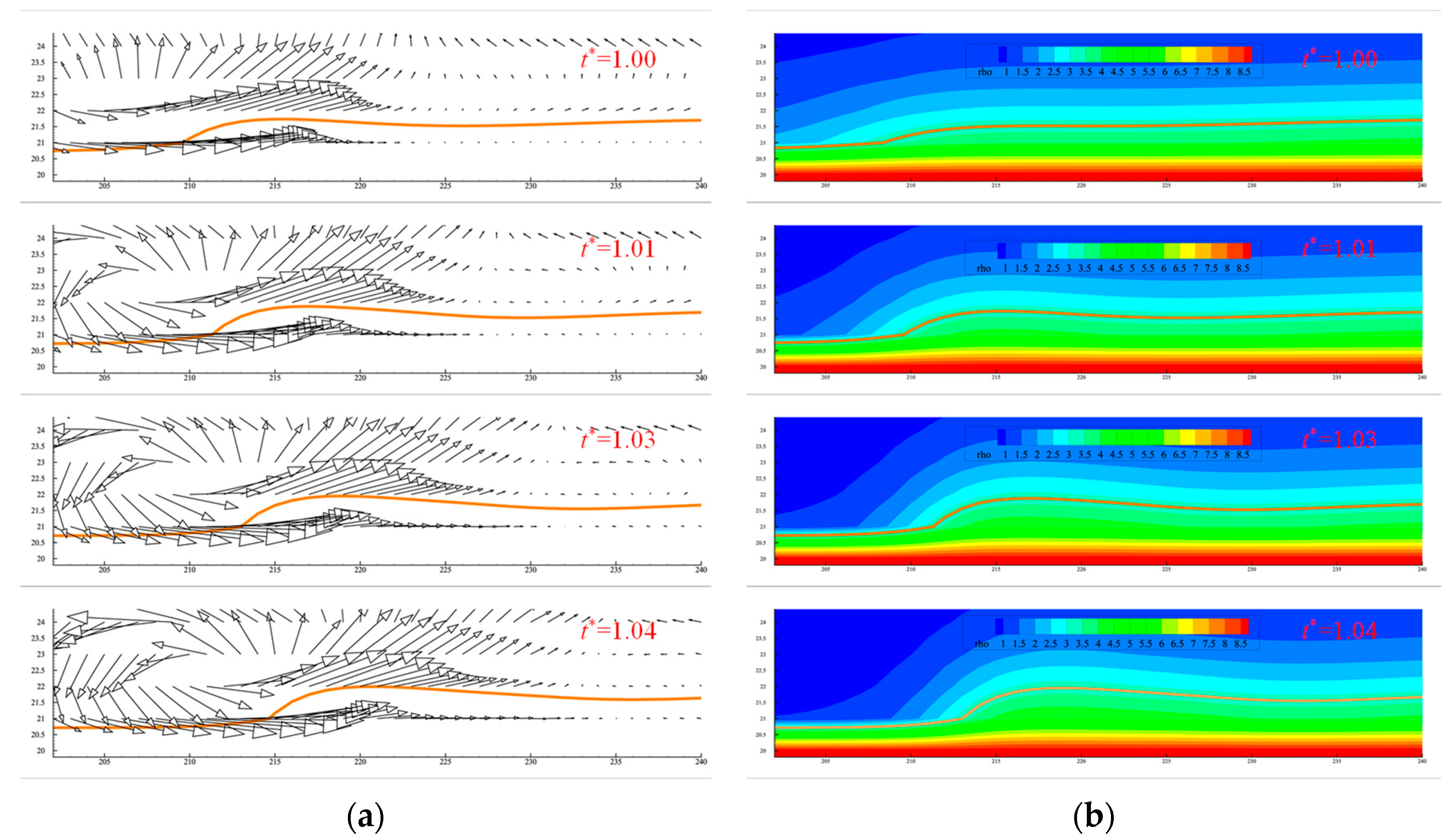
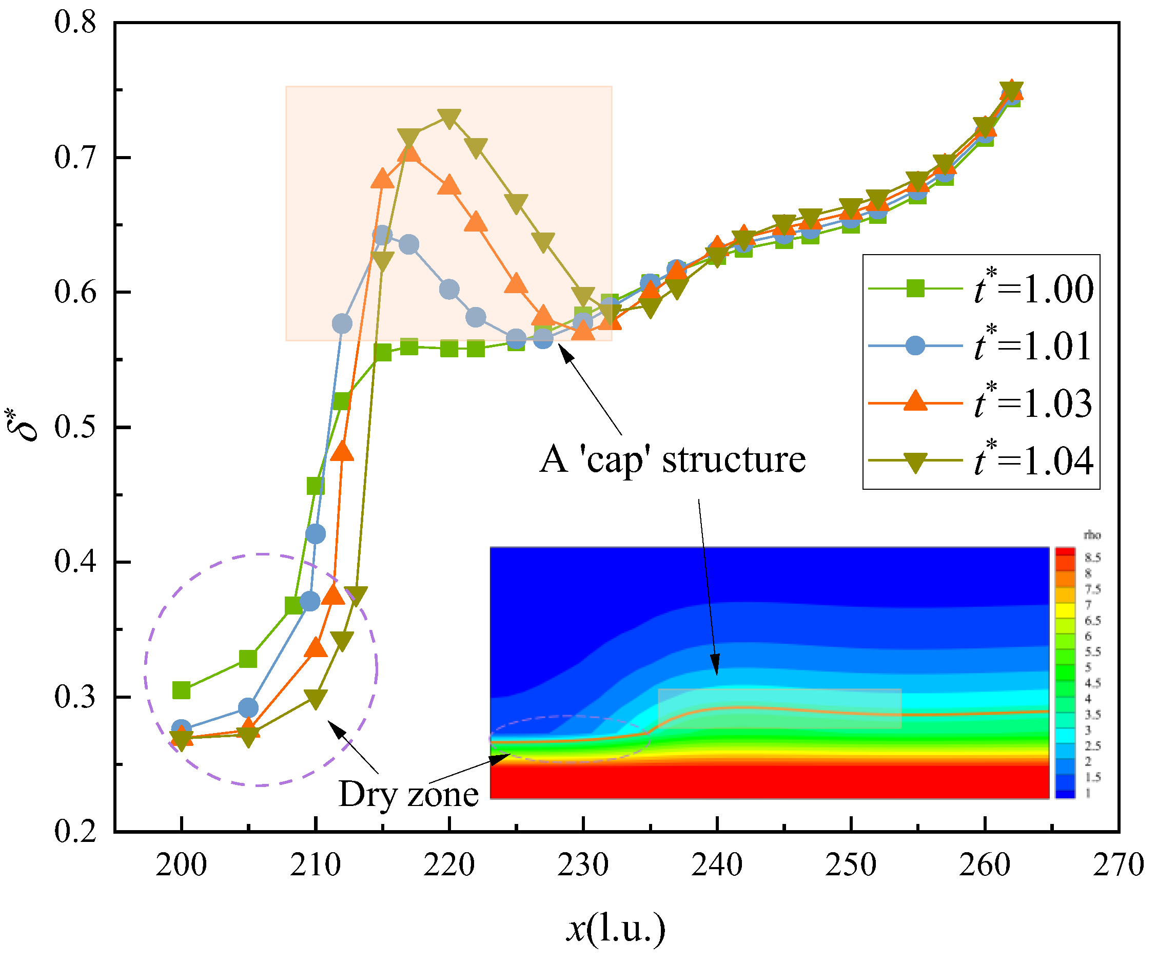
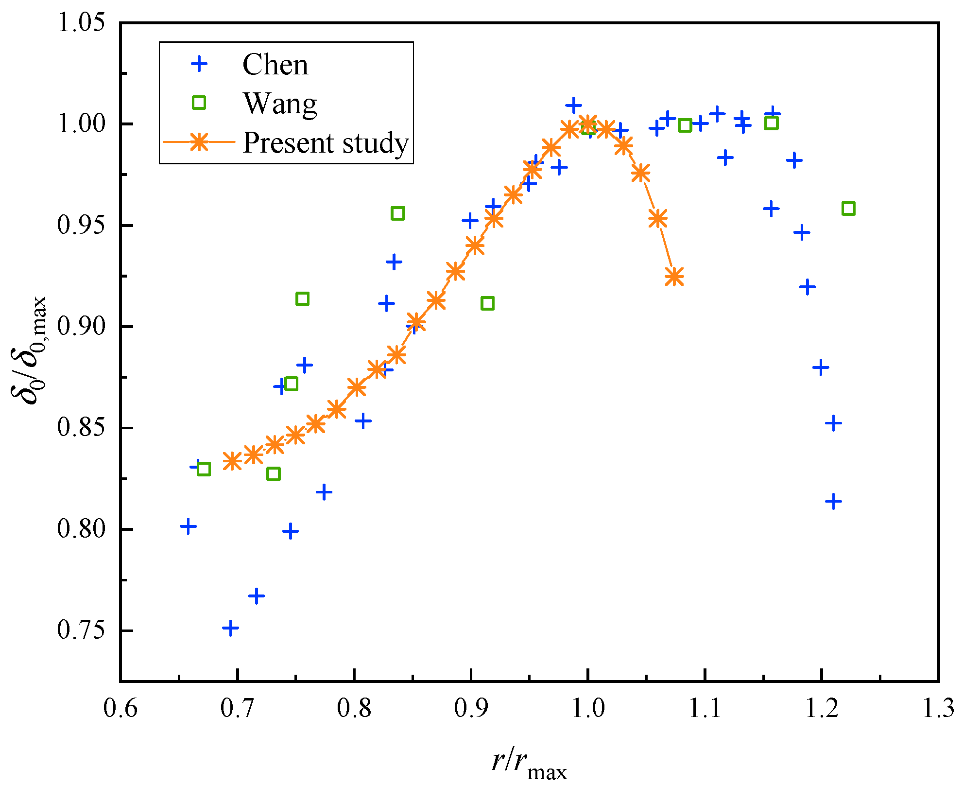
During the evaporation process, the microlayer displays a contraction behavior due to the differences in flow rate in different areas, especially at the three-phase contact point, where the difference in flow rate is larger than that in other places, leading to the accumulation of microlayer heads and the formation of a “cap-like” structure. The growth of the dry zone shows a linear pattern at the beginning; then, with the increase in the microlayer’s thickness, the growth of the dry spot slows down, and the change starts to become flat. Due to the effect of the density of the near-wall surface, there is also a certain thickness of the dry zone. The initial microlayer thickness was compared with previous studies, showing a consistent trend. However, some differences exist due to the inherent disparities between experimental and numerical simulations.

(2)

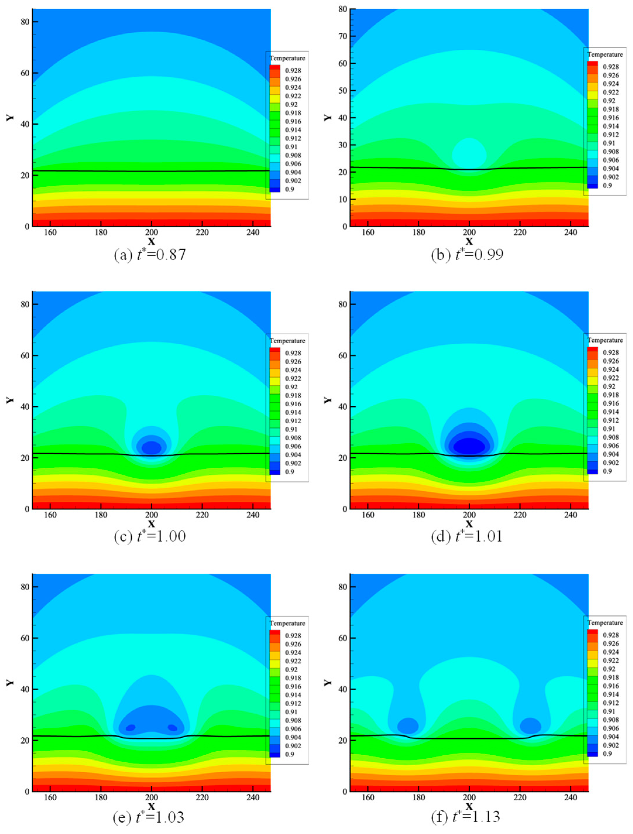
During the study of heat flux, the lowest heat flux at the three-phase contact point occurred when dry spots appeared and there was a sudden increase in heat flux. After the appearance of the dry spot, the heat flux at the three-phase contact point was the lowest. At the time of the dry spot, a cold air ring appeared above the dry zone, and it expanded and then split, moving with the three-phase contact point.

(3)

Raising the temperature is beneficial to the microlayer evaporation process. Under the condition of Hs = 1,400,000 and the same heating duration, increasing the temperature from T = 0.93 T_cr to T = 0.94 T_cr raises the evaporation volume by 3.2% and 6.7% compared to T = 0.935 T_cr and T = 0.93 T_cr, respectively, reduces the total fluid mass to 0.868 (compared to 0.881 and 0.894, respectively), and, through the synergistic action of internal and external Marangoni effects, leads to an approximately linear increase in evaporation volume and a linear decrease in total mass.

References

1. Zhao, Y.H.; Masuoka, T.; Tsuruta, T.J.I.J.o.H.; Transfer, M. Unified theoretical prediction of fully developed nucleate boiling and critical heat flux based on a dynamic microlayer model. Int. J. Heat Mass Transf. 2002, 45, 3189–3197. [Google Scholar] [CrossRef]
2. Utaka, Y.; Kashiwabara, Y.; Ozaki, M.; Chen, Z. Heat transfer characteristics based on microlayer structure in nucleate pool boiling for water and ethanol. Int. J. Heat Mass Transf. 2014, 68, 479–488. [Google Scholar] [CrossRef]
3. Utaka, Y.; Kashiwabara, Y.; Ozaki, M. Microlayer structure in nucleate boiling of water and ethanol at atmospheric pressure. Int. J. Heat Mass Transf. 2013, 57, 222–230. [Google Scholar] [CrossRef]
4. Liu, Z.; Wei, J.; Gong, S.; Cheng, P. High fidelity simulations of single bubble nucleate boiling heat transfer considering microscale effects. Int. J. Heat Mass Transf. 2025, 239, 126584. [Google Scholar] [CrossRef]
5. Sodtke, C.; Kern, J.; Schweizer, N.; Stephan, P. High resolution measurements of wall temperature distribution underneath a single vapour bubble under low gravity conditions. Int. J. Heat Mass Transf. 2006, 49, 1100–1106. [Google Scholar] [CrossRef]
6. Gao, M.; Zhang, L.; Cheng, P.; Quan, X. An investigation of microlayer beneath nucleation bubble by laser interferometric method. Int. J. Heat Mass Transf. 2013, 57, 183–189. [Google Scholar] [CrossRef]
7. Chen, Z.; Haginiwa, A.; Utaka, Y. Detailed structure of microlayer in nucleate pool boiling for water measured by laser interferometric method. Int. J. Heat Mass Transf. 2017, 108, 1285–1291. [Google Scholar] [CrossRef]
8. Tecchio, C.; Cariteau, B.; Houedec, C.L.; Bois, G.; Saikali, E.; Zalczer, G.; Vassant, S.; Roca i Cabarrocas, P.; Bulkin, P.; Charliac, J.; et al. Microlayer evaporation during bubble growth in nucleate boiling. Int. J. Heat Mass Transf. 2024, 231, 125860. [Google Scholar] [CrossRef]
9. Han, J.; Kim, I.; Choi, J.; Kim, H. Contribution of wall heat transfer in the transition region between microlayer and macroscopic regions to the growth of a single boiling bubble. Int. J. Heat Mass Transf. 2024, 235, 126213. [Google Scholar] [CrossRef]
10. Sato, Y.; Niceno, B. A depletable micro-layer model for nucleate pool boiling. J. Comput. Phys. 2015, 300, 20–52. [Google Scholar] [CrossRef]
11. Giustini, G.; Jung, S.; Kim, H.; Ardron, K.H.; Walker, S.P. Microlayer evaporation during steam bubble growth. Int. J. Therm. Sci. 2019, 137, 45–54. [Google Scholar] [CrossRef]
12. Gao, M.; Dong, W.h.; Shen, Z.X.; Zhang, L.x. Theoretical model of microlayer and macrolayer evaporation considering heating surface temperature radial distribution at the bottom of the bubble. Int. Commun. Heat Mass Transf. 2023, 140, 106515. [Google Scholar] [CrossRef]
13. Chen, Z.; Utaka, Y. On heat transfer and evaporation characteristics in the growth process of a bubble with microlayer structure during nucleate boiling. Int. J. Heat Mass Transf. 2015, 81, 750–759. [Google Scholar] [CrossRef]
14. Chen, Z.; Wu, F.; Utaka, Y. Numerical simulation of thermal property effect of heat transfer plate on bubble growth with microlayer evaporation during nucleate pool boiling. Int. J. Heat Mass Transf. 2018, 118, 989–996. [Google Scholar] [CrossRef]
15. Zhang, J.; Rafique, M.; Ding, W.; Bolotnov, I.A.; Hampel, U. Direct numerical simulation of microlayer formation and evaporation underneath a growing bubble driven by the local temperature gradient in nucleate boiling. Int. J. Therm. Sci. 2023, 193, 108551. [Google Scholar] [CrossRef]
16. Wang, J.; Wang, Z.; He, S.; Li, B.; Wang, J. Marangoni effect on the size of dry spot and CHF in saturated pool boiling of pure water and RB solution. Int. Commun. Heat Mass Transf. 2023, 141, 106601. [Google Scholar] [CrossRef]
17. Girimaji, S. Lattice Boltzmann Method: Fundamentals and Engineering Applications with Computer Codes. AIAA J. 2013, 51, 278–279. [Google Scholar] [CrossRef]
18. Yang, J.h.; Gao, M.; Wang, D.m.; Dong, W.h.; Zuo, Q.r. Lattice Boltzmann simulation of the effect for adding a ghost fluid layer on the simulation accuracy of a sessile droplet on a heated surface. Int. J. Therm. Sci. 2023, 193, 108525. [Google Scholar] [CrossRef]
19. He, X.; Luo, L.S. Theory of the lattice Boltzmann method: From the Boltzmann equation to the lattice Boltzmann equation. Phys. Rev. E 1997, 56, 6811–6817. [Google Scholar] [CrossRef]
20. Shi, Y.; Zhao, T.S.; Guo, Z.L. Thermal lattice Bhatnagar-Gross-Krook model for flows with viscous heat dissipation in the incompressible limit. Phys. Rev. E 2004, 70, 066310. [Google Scholar] [CrossRef] [PubMed]
21. Kupershtokh, A.L.; Medvedev, D.A. Lattice Boltzmann equation method in electrohydrodynamic problems. J. Electrost. 2006, 64, 581–585. [Google Scholar] [CrossRef]
22. Gong, S.; Cheng, P. Numerical investigation of droplet motion and coalescence by an improved lattice Boltzmann model for phase transitions and multiphase flows. Comput. Fluids 2012, 53, 93–104. [Google Scholar] [CrossRef]
23. Yuan, P.; Schaefer, L. Equations of state in a lattice Boltzmann model. Phys. Fluids 2006, 18, 42101–42111. [Google Scholar] [CrossRef]
24. Hu, A.; Li, L.; Uddin, R.; Liu, D. Contact angle adjustment in equation-of-state-based pseudopotential model. Phys. Rev. E 2016, 93, 053307. [Google Scholar] [CrossRef]
25. Li, Q.; Luo, K.H.; Kang, Q.J.; Chen, Q. Contact angles in the pseudopotential lattice Boltzmann modeling of wetting. Phys. Rev. E 2014, 90, 053301. [Google Scholar] [CrossRef]
26. Li, Q.; Yu, Y.; Luo, K.H. Implementation of contact angles in pseudopotential lattice Boltzmann simulations with curved boundaries. Phys. Rev. E 2019, 100, 053313. [Google Scholar] [CrossRef]
27. Guo, Z.; Shi, B.; Zheng, C. A coupled lattice BGK model for the Boussinesq equations. Int. J. Numer. Methods Fluids 2002, 39, 325–342. [Google Scholar] [CrossRef]
28. Gong, S.; Cheng, P. A lattice Boltzmann method for simulation of liquid–vapor phase-change heat transfer. Int. J. Heat Mass Transf. 2012, 55, 4923–4927. [Google Scholar] [CrossRef]
29. Li, Q.; Zhou, P.; Yan, H.J. Improved thermal lattice Boltzmann model for simulation of liquid-vapor phase change. Phys. Rev. E 2017, 96, 063303. [Google Scholar] [CrossRef]
30. Zhang, C.; Cheng, P. Mesoscale simulations of boiling curves and boiling hysteresis under constant wall temperature and constant heat flux conditions. Int. J. Heat Mass Transf. 2017, 110, 319–329. [Google Scholar] [CrossRef]
31. Nemati, M.; Shateri Najaf Abady, A.R.; Toghraie, D.; Karimipour, A. Numerical investigation of the pseudopotential lattice Boltzmann modeling of liquid–vapor for multi-phase flows. Phys. A Stat. Mech. Its Appl. 2018, 489, 65–77. [Google Scholar] [CrossRef]
32. Lakew, E.; Sarchami, A.; Giustini, G.; Kim, H.; Bellur, K. Thin Film Evaporation Modeling of the Liquid Microlayer Region in a Dewetting Water Bubble. Fluids 2023, 8, 126. [Google Scholar] [CrossRef]
33. Wang, J.; Wang, H.; Xiong, J. Experimental investigation on microlayer behavior and bubble growth based on laser interferometric method. Front. Energy Res. 2023, 11, 1130459. [Google Scholar] [CrossRef]
Figure 1. Young–Laplace law verification.
Processes 13 00872 g001
Figure 2. Variation in the droplet diameter ratio with heating time.
Processes 13 00872 g002
Figure 3. Grid independence verification: (a) Microlayer profile at the initial moment of dry spot formation under different grid resolutions. (b) Temperature distribution along the microlayer boundary at the initial moment of dry spot formation under different grid resolutions.
Processes 13 00872 g003
Figure 4. Liquid layer model.
Processes 13 00872 g004
Figure 5. Microlayer head change: (a) Velocity field around the microlayer during evaporation. (b) Density of microlayers during evaporation.
Processes 13 00872 g005
Figure 6. Variation in dry spot radius with dimensionless time.
Processes 13 00872 g006
Figure 7. Dimensionless thickness at different x.
Processes 13 00872 g007
Figure 8. Plot of the initial microlayer thickness.
Processes 13 00872 g008
Figure 9. Graph of temperature phenomena during evaporation.
Processes 13 00872 g009
Figure 10. Heat flux distribution of the microlayer: (a) before and at the appearance of the dry spot; (b) after the appearance of the dry spot.
Processes 13 00872 g010
Figure 11. Evaporation at different temperatures.
Processes 13 00872 g011
Figure 12. Total fluid mass at different temperatures.
Processes 13 00872 g012
Figure 13. Marangoni vortex outside the microlayer.
Processes 13 00872 g013
Disclaimer/Publisher’s Note: The statements, opinions and data contained in all publications are solely those of the individual author(s) and contributor(s) and not of MDPI and/or the editor(s). MDPI and/or the editor(s) disclaim responsibility for any injury to people or property resulting from any ideas, methods, instructions or products referred to in the content.