Numerical Analysis of the Flame-Arresting Performance of a Pipeline Flame Arrester

Abstract

This research aims to create a numerical model for analyzing the flame propagation and quenching mechanisms of a pipeline flame arrester. Based on fundamental theories of flame propagation and quenching, a numerical model is established and solved using Ansys Workbench. The model accuracy is verified by comparing numerical results with experimental data. The verified model enables detailed flow field analysis. Using this validated model, a detailed flow field analysis is conducted. The temperature field and chemical reaction rate distribution under practical working conditions are analyzed. A method for determining the quenching length is established. The effects of flame arrester porosity, flame arrester core thickness, inlet flame velocity, and flame arrester length on the quenching length are analyzed. The Box-Behnken response surface method is applied to predict the quenching length. This approach produces an accurate prediction equation. These results can help improve flame arrester design and strengthen safety performance.

1. Introduction

Pipeline flame arresters are critical devices designed to prevent flame propagation in pipeline systems. Pipeline flame arresters are widely used in industries such as oil, natural gas, chemicals, and other industrial pipelines [1]. With the advancement of industrialization and increasing safety demands, pipeline flame arresters have become an important research area. According to the relevant literature, the main goal of pipeline flame arresters is to effectively suppress the spread of flames. Pipeline flame arresters prevent the fire from spreading while keeping the fluid flowing in the pipeline [2].

Current research on pipeline flame arresters can be classified into three main areas: theoretical studies, experimental testing, and numerical simulations. Theoretical research mainly focuses on the analysis of the flame-quenching mechanism. Two main categories have emerged. One is the cold-wall effect theory, and the other is the wall effect theory [3]. However, due to the complex chemical reactions and multi-physical-field coupling involved in the actual process, existing theoretical models still need to be further improved to more accurately describe the flame-quenching process.

Experimental research provides critical support for validating theoretical models and optimizing flame arrester designs. Bao et al. [4] studied in-line detonation flame arresters. With a DN50 apparatus and a 6.6% C₂H₄–air mixture, they found pressure and velocity attenuation related to filter thickness. Two fire-extinguishing failure modes were identified. Cao et al. [5] used a visual system to explore a corrugated flame arrester’s resistance in hydrogen explosions. By varying the structural parameters and hydrogen concentration, they noted a link between flame propagation and pressure rise. Overall, experimental studies on flame arresters have provided valuable insights into their effectiveness in preventing flame propagation and explosions in industrial settings. However, experiments are costly, especially when simulating extreme conditions like high pressure and large flow rates. The safety and accuracy of experimental equipment become significant constraints [6].

With the development of computational fluid dynamics (CFD) technology, numerical simulation has been widely applied in flame arrester research. Numerical simulation research can be classified into two types. One is to study the material properties of flame arresters or pipeline systems under high-temperature conditions. Fonseca et al. [7] developed a finite element algorithm to perform the thermal and mechanical analysis of structural steel piping systems subjected to elevated temperatures. Zong et al. [8] proposed numerical material models for steel and mineral wool. The temperature distribution and structural deformation were simulated using Abaqus. The other type is to study the propagation characteristics of flames and the hydrodynamic characteristics of fluids within flame arresters or pipelines. Yue et al. [9] proposed a novel detonation arrester structure for large pipelines, based on heat transfer theory. The monolithic structure, composed of a large disk with long triangular slits, was analyzed for quenching characteristics and verified by simulation. Liu et al. [10] numerically modeled premixed gas propagation in a pipeline flame arrester. They found distinct flame propagation and pressure change patterns for propane–air, ethylene–air, and hydrogen–air mixtures. The effect of initial pressure on explosion pressure and flame propagation rate was also studied. Farah et al. [11] used a porous media model to numerically study the flow in a crimped flame arrester. Empirical coefficients in the Forchheimer equation were determined via small-scale tests. The model was verified with experimental data, then applied to a larger-scale arrester.

At present, the standards and specifications guiding the design of flame arresters are not perfect [1]. Existing research lacks comprehensive and in-depth exploration of the complex physical processes within flame arresters. As a result, the design of flame arresters often fails to achieve optimal performance under diverse working conditions. Numerical simulation has emerged as an effective approach for researching pipeline flame arresters. In this study, with the quenching length taken as a key parameter, numerical simulation methods are combined to conduct research on the flame-blocking performance. This approach aims to contribute to a more in-depth understanding of the flame-blocking mechanisms of pipeline flame arresters. A predictive model of quenching length based on the Box–Behnken response surface method is applied. It enables the development of more efficient and reliable flame arresters.

2. Physical Structure

The pipeline flame arrester commonly used in natural gas transmission stations is shown in Figure 1. The pipeline flame arrester is composed of an arrester housing and an arrester element, along with other related fittings. As the flame traverses the arrester, it infiltrates the microchannels of the arrester element. These microchannels are made up of numerous isosceles-trapezoid micro-structures. Simultaneously, the flame is fragmented into smaller flamelets. Owing to the high-efficiency heat absorption capacity of these microchannels, the flame can be effectively quenched.

The quenching mechanism of the flame arrester unit is mainly heat conduction. When the medium passes through the region of the flame arrester unit, a certain pressure difference will occur at both ends of the region. The magnitude of this pressure difference is jointly influenced by the structure of the flame arrester unit and the medium flow rate. Therefore, in this study, the region of the flame arrester unit within the pipeline is treated as a unified porous medium region. The flame arrester configuration is depicted in Figure 1. Pipelines of nominal diameter DN60 and length 400 mm are, respectively, connected to two extremities of the flame arrester. As a consequence, the internal flow field domain of the pipeline flame arrester is established, as illustrated in Figure 2.

3. Mathematical Model

3.1. Governing Equations

In the control volume, the principles of conservation governing continuity, momentum, and energy are upheld. These mathematical models, which encapsulate these fundamental conservation laws, can be formulated through the subsequent equations.

(1)

Continuity equation

The continuity equation is presented as Equation (1).

$${\displaystyle \frac{\partial \rho }{\partial t}}+u{\displaystyle \frac{\partial \left(\rho u\right)}{\partial x}}+v{\displaystyle \frac{\partial \left(\rho v\right)}{\partial y}}+w{\displaystyle \frac{\partial \left(\rho w\right)}{\partial z}}=0$$

(1)

where t is the time and ρ is the density. u, v, w are the components of velocity along the x-axis, y-axis, and z-axis, respectively.

(2)

Momentum equation

For compressible viscous fluids, the momentum conservation equation is presented as Equation (2).

$${\displaystyle \frac{\partial }{\partial t}}(\rho \overrightarrow{v})+\nabla \cdot (\rho \overrightarrow{v}\overrightarrow{v})=-\nabla P+\nabla \cdot (\overrightarrow{\overrightarrow{\tau }})$$

(2)

where P is the pressure. $\overrightarrow{\overrightarrow{\tau }}$ is the stress tensor, and its expression is shown in Equation (3).

$$\overrightarrow{\overrightarrow{\tau }}=\mu \left(\nabla \overrightarrow{v}-{\displaystyle \frac{2}{3}}\nabla \cdot \overrightarrow{v}I\right)$$

(3)

where μ is the dynamic viscosity of the fluid and I is the unit tensor.

(3)

Energy equation

The flame-arresting process has heat exchange phenomena. It is necessary to observe the law of energy conservation. The mathematical formulation of this law is presented as Equation (4).

$${\displaystyle \frac{\partial \left(\rho T\right)}{\partial t}}+{\displaystyle \frac{\partial }{\partial x_i}}\left(\rho u_{i}T\right)={\displaystyle \frac{\partial }{\partial x_i}}\left({\displaystyle \frac{\lambda }{C_p}}{\displaystyle \frac{\partial T}{\partial x_i}}\right)+{\displaystyle \frac{1}{C_P}}{\displaystyle \frac{\partial P}{\partial t}}+{\displaystyle \frac{h_c}{C_P}}{R}_{fu,A}$$

(4)

where T is the temperature, λ is the thermal conductivity, C_p is the heat capacity, h_c is the heat of combustion, and R_fu,A is the reaction activity rate of the component.

(4)

Species conservation equation

Within systems characterized by mass exchange or the presence of a multitude of chemical constituents, each component is required to follow the law of mass conservation. This principle describes how a specific chemical species in the system changes over time. The mathematical formulation of the component conservation equation is expressed as Equation (5).

$$\left\{\begin{array}{l}{\displaystyle \frac{\partial \left(\rho y_f\right)}{\partial t}}+{\displaystyle \frac{\partial }{\partial x_i}}\left(\rho u_i,y_f\right)={\displaystyle \frac{\partial }{\partial x_i}}\left(D\rho {\displaystyle \frac{\partial y_f}{\partial x_i}}\right)-R_{fu,A}\\ {\displaystyle \frac{\partial \left(\rho y_o\right)}{\partial t}}+{\displaystyle \frac{\partial }{\partial x_i}}\left(\rho u_i,y_o\right)={\displaystyle \frac{\partial }{\partial x_i}}\left(D\rho {\displaystyle \frac{\partial y_o}{\partial x_i}}\right)-s{R}_{fu,A}\\ {\displaystyle \frac{\partial \left(\rho y_p\right)}{\partial t}}+{\displaystyle \frac{\partial }{\partial x_i}}\left(\rho u_i,y_p\right)={\displaystyle \frac{\partial }{\partial x_i}}\left(D\rho {\displaystyle \frac{\partial y_p}{\partial x_i}}\right)-\left(s+1\right)R_{fu,A}\end{array}\right.$$

(5)

where u_i is the velocity in each direction. y is the mass concentration. The subscripts f, o, and y represent fuel, oxygen, and products, respectively. D is the diffusion coefficient, and s is the mass stoichiometric ratio.

3.2. Turbulence Model

The standard k-ε turbulence model has a wide range of applications. In the context of the present study, the phenomena of flame propagation and quenching can be classified as typical general flows. The standard k-ε model is chosen to describe the turbulent attributes inherent in the combustion process [12].

3.3. Combustion Model

A crucial aspect of the combustion model involves the determination of the turbulent combustion rate, denoted as R_fu. Numerous studies have confirmed that the EBU–Arrhenius model is effective in characterizing the turbulent combustion rate during the combustion process [13]. Within the framework of the EBU–Arrhenius model, the laminar reaction and turbulent fluctuation are two pivotal mechanisms that affect the combustion reaction rate [14].

The calculation formula for the turbulent combustion rate is shown in Equation (6).

$$R_{fu}=-\min \left(\left|R_{fu,A}\right|,\left|R_{fu,T}\right|\right)$$

(6)

where R_fu,A is the Arrhenius-type combustion rate and R_fu,T is the turbulent combustion rate. R_fu,A and R_fu,T are presented as Equations (7) and (8), respectively.

$$R_{fu,A}=B{\rho }^2{Y}_1{Y}_2\exp \left(-{\displaystyle \frac{E_a}{RT}}\right)$$

(7)

$$R_{fu,T}=C_{EBU}\rho {\displaystyle \frac{\epsilon }{k}}\min \left(Y_1,Y_2,Y_3\right)$$

(8)

where B is the pre-exponential factor. C_EBU is an empirical constant, and its value typically ranges from 0.34 to 0.4. E_a is the activation energy. R is the gas constant. Y is the mass fraction. The subscripts 1, 2, and 3 represent fuel, oxygen, and combustion products, respectively.

3.4. Porous Media Model

Within the porous media model, the continuity equation is expressed as Equation (9).

$${\displaystyle \frac{\partial \left(\gamma \rho \right)}{\partial t}}+\nabla \cdot \left(\gamma \rho \overrightarrow{u}\right)=0$$

(9)

where γ is the porosity of porous media and ρ is the fluid density.

In the momentum equation of the porous medium, the additional momentum source term is composed of the viscous loss term and the inertial loss term. The expression is shown as Equation (10).

$$S_i=-\left({\displaystyle \sum _{j=1}^3{D}_{ij}\mu v_j}+{\displaystyle \sum _{j=1}^3{C}_{ij}\frac{1}{2}\rho \left|v_j\right|v_j}\right)$$

(10)

where S_i is the momentum source term in the i-th direction. D is the diffusion coefficient matrix, and C is the resistance coefficient matrix.

Considering the properties of the flame arrester core, Equation (10) can be transformed into the form of Equation (11).

$$S_i=-\left({\displaystyle \frac{\mu }{\alpha }}{v}_i+C_2{\displaystyle \frac{1}{2}}\rho \left|v_j\right|v_j\right)$$

(11)

where 1/α is the viscous drag coefficient. C₂ is the inertial drag coefficient. The matrices D and C are simplified to diagonal matrices. The diagonal elements of these matrices are assigned the values of 1/α and C₂, respectively. All non-diagonal elements are set to zero.

The modification of the convective and transient terms in the governing equations gives rise to the porous-medium energy equation, as presented in Equation (12). This equation can describe the energy transfer process in the porous medium more accurately.

$$\begin{array}{l}{\displaystyle \frac{\partial }{\partial t}}\left(\gamma {\rho }_f{E}_f+\left(1-\gamma \right){\rho }_s{E}_s\right)+\nabla \cdot \left(\overrightarrow{v}\left({\rho }_f{E}_f+P\right)\right)\\ =\nabla \cdot \left[k_{eff}\nabla T-\left({\displaystyle \sum _i{h}_i{J}_i}\right)+\left(\overrightarrow{\overrightarrow{\tau }}\cdot \overrightarrow{v}\right)\right]+S_f^h\end{array}$$

(12)

where E_f is the total energy of the fluid, and E_s is the total energy of the solid medium. ρ_f is the density of the fluid, and ρ_s is the density of the solid medium. k_eff is the effective thermal conductivity coefficient, and S is the source term.

In order to more precisely unveil the heat transfer mechanism in the combustion process, the non-equilibrium energy equation is adopted for the solution. The temperatures of the fluid region and the solid region are calculated separately.

4. Numerical Methods

4.1. Boundary Conditions and Initial Conditions

In this study, some assumptions are made during the solution process of the established simulation calculation model of the flame arrester. The reaction in which methane burns with oxygen to produce gaseous water and carbon dioxide is irreversible. The nitrogen has no effect on the reaction. It is assumed that the wall has no thickness. The standard wall function is adopted. There is no slip on the wall surface. During the simulation calculation of flame arrestment, the effect of radiative heat transfer is not considered.

The flame-arresting unit is defined as a porous region. The porosity which affects the velocity scaling should be given. Based on the characteristics of the porous medium, the viscous drag coefficient and inertial drag coefficient are calculated. Then, the coefficients are put into viscous and inertial resistance fields in the software. The basic parameters of flame-arresting unit for the simulation are shown in

Table 1. Fire-retardant unit parameter settings [11].

Parameter Name	Value
Thickness of the flame arrester unit (mm)	140
Porosity	0.8
Viscous drag coefficient (in the X direction)	1.66 × 106
Viscous drag coefficient (in the Y direction)	1.66 × 109
Viscous drag coefficient (in the Z direction)	1.66 × 109
Inertial drag coefficient (in the X direction)	223,278
Inertial drag coefficient (in the Y direction)	223,278
Inertial drag coefficient (in the Z direction)	223,278

.

Regarding the inlet boundary conditions, a velocity inlet is specified with a constant velocity. The temperature at the inlet is set to the adiabatic combustion temperature of the methane–air mixture. For the outlet boundary conditions, a pressure outlet is employed with the pressure maintained at normal atmospheric pressure. The initial temperature at the outlet is set to 300 K. The composition of the gas mixture consists of 23% oxygen and 77% nitrogen. The wall surface is configured as a constant-temperature wall.

For the initial conditions, it is assumed that a small area near the closed end is the burned zone. The adiabatic combustion temperature of the burned zone is set to 2323 K. The initial conditions for the gas mixture are configured as presented in

Table 2. Setting of initial conditions for methane–air premixed flame.

Methane–Air Mixture	Unburned Zone	Burned Zone
T	300 K	2323 K
P0	101,325 Pa	101,325 Pa
YO2	22%	0
YCH4	15%	0
YH2O	0	11%
YCO2	0	15.5%

.

After initializing the computational domain, an ignition strategy is used. It introduces energy into a defined sub-region. This sub-region is called the burned zone, and its temperature is set to 2323 K. Concurrently, a specific quantity of reaction products is introduced into this zone to initiate the reaction. During the iterative process, the temperature of the burned zone is automatically adjusted to the temperature characteristic of normal methane combustion. This approach ensures the simulation’s rationality and accuracy.

4.2. Solution Method

The Ansys Workbench 19.2 is used to solve the mathematical model. To accurately discretize the convective terms present in all the governing equations, a second-order upwind scheme is implemented. The SIMPLE (Semi-Implicit Method for Pressure-Linked Equations) algorithm is adopted to deal with the pressure–velocity coupling [15]. A three-dimensional (3D) segregated solver, integrated with the under-relaxation method, is employed to solve the system of conservation equations. For all equations involved in the simulation, the convergence criteria for the residuals are set to a highly stringent value of 1.0 × 10⁻⁶.

4.3. Mesh Generation

Based on the structural characteristics of the flame arrester model, an O-type partitioning method is selected to perform structured grid division on the model. The result of the grid division is shown in Figure 3.

Multiple grids with different densities are generated for the flame arrester model. Four distinct grid configurations are considered, with the number of grid nodes set to 59,092, 33,892, 18,720, and 12,046, respectively. For each grid configuration, a numerical simulation is carried out to model the propagation of a methane–air mixture flame within the flame arrester. The temperature distribution on the central axis of the flame arrester at a specific time (1 ms) is chosen as the evaluation parameter. As shown in Figure 4, when the number of grid nodes is 59,092 and 33,892, respectively, the corresponding calculation results exhibit a high degree of similarity. In contrast, when the number of grid nodes is 12,046 and 18,720, there are significant discrepancies in the corresponding calculation results. The accuracy of the calculation results improves with an increase in the number of grid nodes. However, this improvement comes at the cost of an extended calculation time. Therefore, taking both the calculation results and the calculation time into consideration, a grid with 33,892 nodes is selected as the optimal grid number.

5. Results and Discussion

5.1. Validation

In order to verify the effectiveness of the numerical model in this study, the flame-arresting experimental parameters from Cui [16] were used to conduct numerical simulations. The settings of the simulation parameters are presented in

Table 3. Simulation parameter settings [16].

Simulation Parameters	Parameter Value
Inlet flame velocity (m/s)	10, 20, 30, 40, 50, 60
Porosity	0.8
YO2 (inlet)	22%
YCH4 (inlet)	15%
YH2O (inlet)	0
YCO2 (inlet)	0
YO2 (outlet)	0
YCH4 (outlet)	0
YH2O (outlet)	11%
YCO2 (outlet)	15.5%
Inlet ignition temperature (K)	2323
Outlet pressure (Pa)	101,325

.

The comparison between the pressure drop values obtained under different velocity conditions and the experimental results is shown in Figure 5. It can be seen that the results of the numerical simulation are in good agreement with the experimental results. The error is no more than 3%. This demonstrates that the established numerical calculation model can be used to study the performance of flame arresters.

5.2. Temperature Criterion for Flame Quenching

Establishing the criterion for flame extinction is a crucial issue. After years of research, scholars have introduced the Peclet number (Pe number) to accurately determine the extinction status of gas flames. The Pe number as a key indicator provides a powerful tool for solving this problem.

The Pe number is calculated according to Equation (13).

$$Pe=S_u{d}_{cr}/\alpha$$

(13)

where d_cr is the quenching diameter, S_u is the adiabatic premixed flame speed, and α is the thermal diffusivity of the unburned gas.

The Pe number was first proposed by Adler and Spalding [17] in 1961. The Pe number is the ratio of convective heat transfer to heat conduction. It reflects the quenching characteristics of the flame under specific conditions. The larger the Pe number, the more prone the flame is to quenching.

The Pe number can effectively measure the difficulty level of flame quenching. Hu [18] discovered that the significant differences in the calculated values of the Pe number are due to the different settings of initial and boundary conditions. However, there is still a lack of a unified standard for the temperatures corresponding to the quenching of different gas flames. Song [19] studied the propagation of combustion flames in parallel slits. When the flame propagation stopped, the temperature in the combustion zone was lower than 1704 K. However, this result is only applicable to premixed acetylene gas flames. Jiang [20] conducted experiments on C-H fuels. It was found that for the combustion reaction to sustain, the temperature of the active radicals generated by the reaction must be at least 1700 K. If the temperature falls below 1700 K, the combustion reaction stops. This means the flame is quenched.

Therefore, in this study, the stable position of the 1700 K isothermal line is taken as the maximum distance that the flame can propagate within the channel. This distance is precisely defined as the quenching length.

5.3. Flow Features

(1)

Temperature field

Numerical simulations of the flame propagation process were carried out based on the initial ignition conditions. The ignition parameters are shown in

Table 4. Simulated operating conditions.

Pipe Diameter	Ignition Method	Initial Pressure	Length of the Ignition End
60 mm	point-by-point ignition	normal pressure	400 mm

.

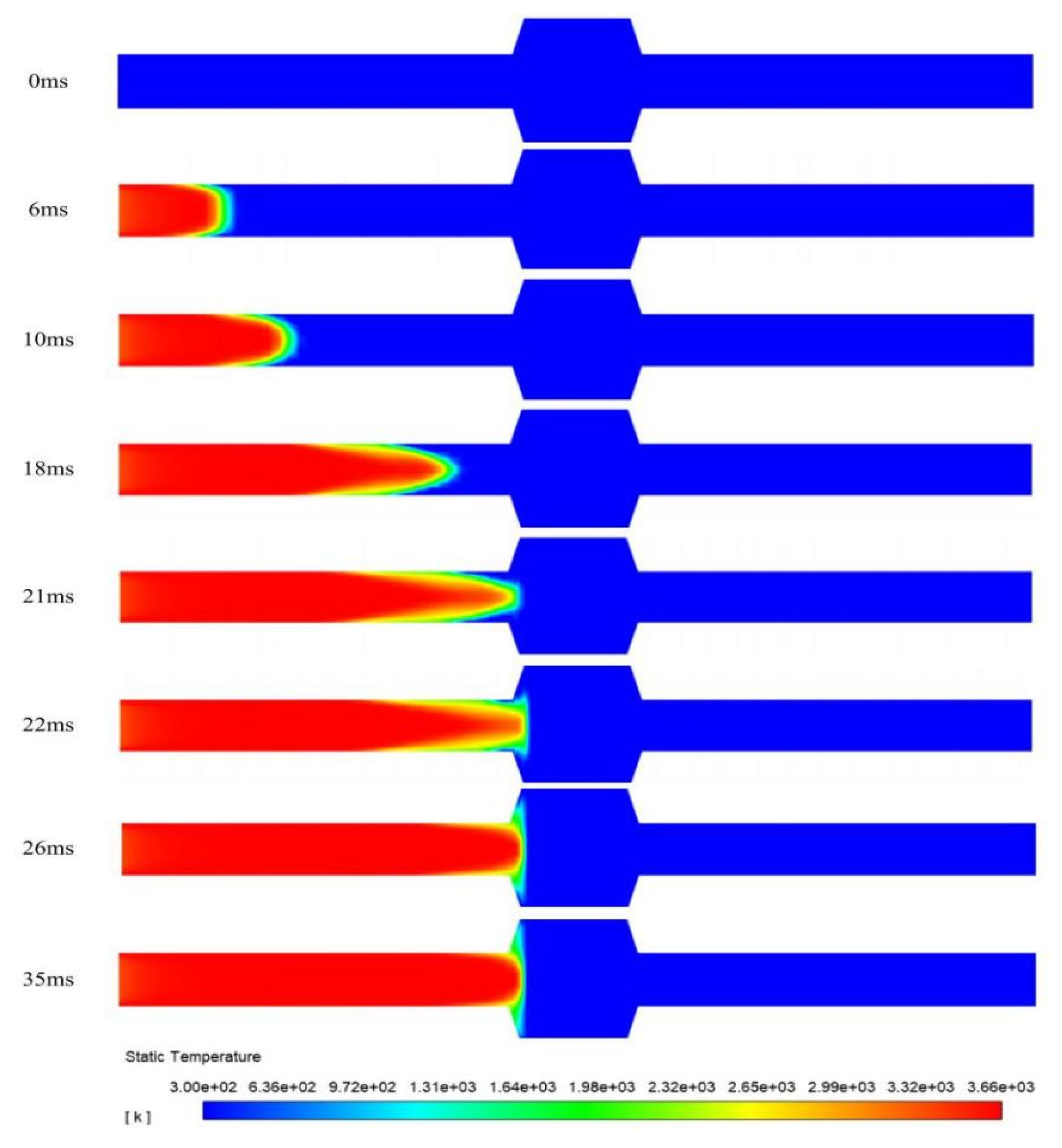
Figure 6 illustrates the propagation process of a deflagration flame within the pipeline. Temperature contour plots of the flame arrester system at different time instants are presented. During the flame propagation stage, at t = 6 ms, the flame has an expanded surface morphology. Its leading edge is hemispherical. The flame front deformation is induced by wall-induced thermal diffusion and viscous effects during propagation. Elongated sharp structures are developed by the initially smooth front. The axial propagation velocities of these structures significantly exceed those in the near-wall regions. By t = 10 ms, the flame transitions into a distinct fingertip configuration. During the quenching stage, at t = 21 ms, the flame front reaches the surface of the flame-arresting element. From t = 21 ms to t = 26 ms, the upstream flame gradually expands in the radial direction. But because of the quenching effect, the flame front near the flame-arresting element keeps stretching. The flame cannot penetrate the flame-arresting element and stays in this region. From t = 26 ms to t = 35 ms, the temperature field shows no significant displacement of the flame front. This means that further flame propagation has been completely suppressed. This proves that the flame arrester can effectively put out the flame under the given conditions.

(2)

Chemical reaction rate field

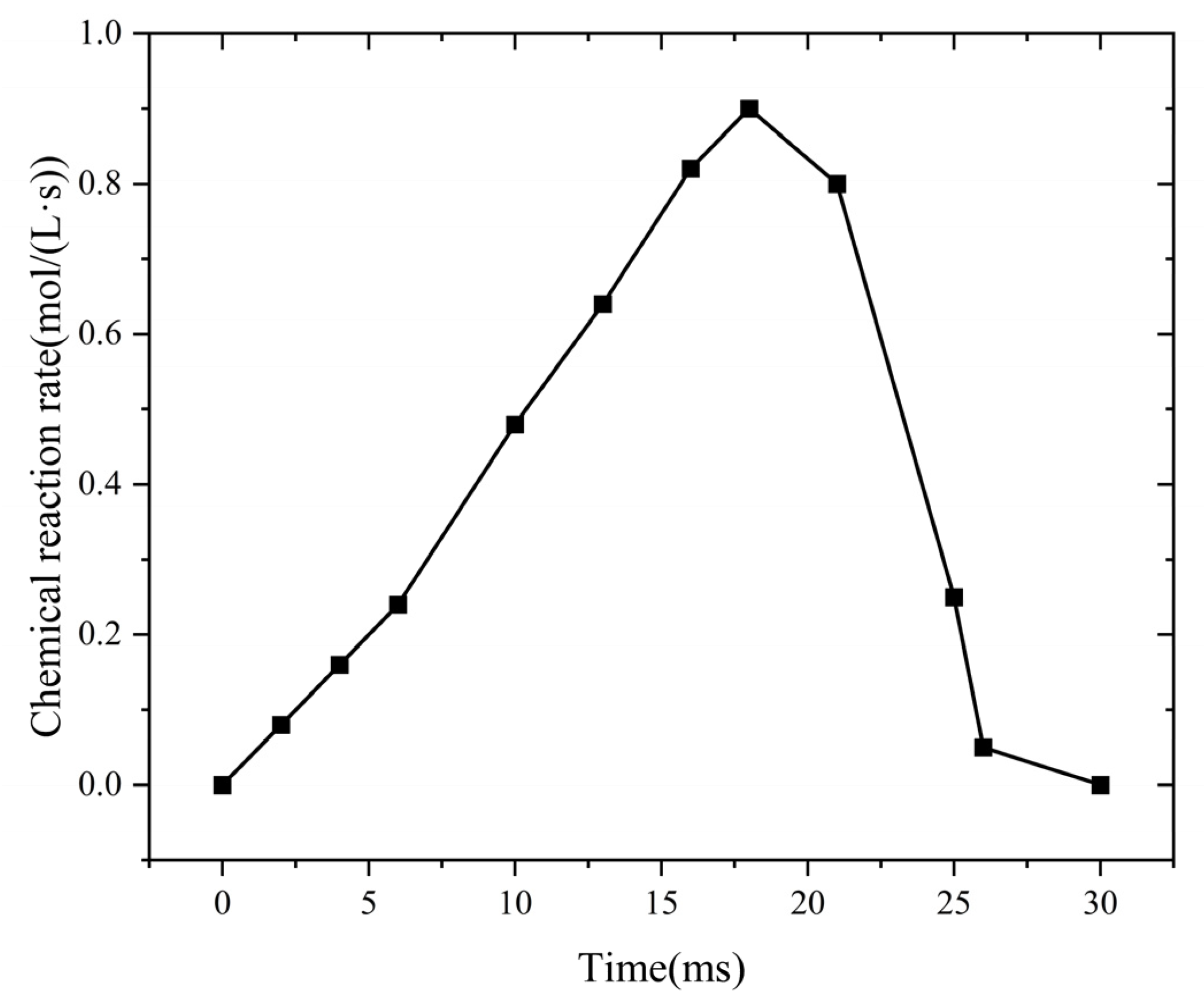
Figure 7 shows the temporal evolution of the chemical reaction rate within the flame-arresting system.

During the flame propagation stage, combustion begins, and the flame advances at a relatively uniform speed. At this point, the chemical reaction rate remains low. As the reaction progresses, the burned gas zone expands quickly. This expansion increases both the flame temperature and propagation speed. Then, the chemical reaction rate rises. During the quenching stage, at t = 21 ms, the flame reaches the flame-arresting element. The temperature of the flame-arresting unit rises gradually. At the same time, the flame temperature decreases. Between t = 21 ms and t = 26 ms, the small pores of the flame-arresting element provide a large specific surface area. This structure improves heat transfer. Heat transfer becomes the main factor in suppressing combustion. Then, the chemical reaction rate drops gradually. After t = 26 ms, the quenching effect spreads throughout the core of the flame-arresting unit. At this point, the chemical reaction rate falls to zero. The flame cannot propagate in the flame-arresting core, indicating that it has been successfully extinguished.

(3)

Analysis of the propagation and quenching processes of deflagration flames

During the flame quenching phase, the intense heat transfer occurring in the channel leads to significant heat loss from the flame as it enters the flame arrester. This rapid heat dissipation results in a substantial reduction in the flame’s temperature. Finally, the flame goes out. When the temperature drops to 1700 K, the C-H fuel cannot produce the active radicals. These radicals are needed for the continuous chemical reaction. As a result, the flame is extinguished due to the absence of these radicals. This shows that the flame quenching in the flame arrester is affected by the combined action of the cold-wall and wall surface effects. The cold-wall effect exerts a predominant influence. The 1700 K isotherm is defined as the flame front boundary. 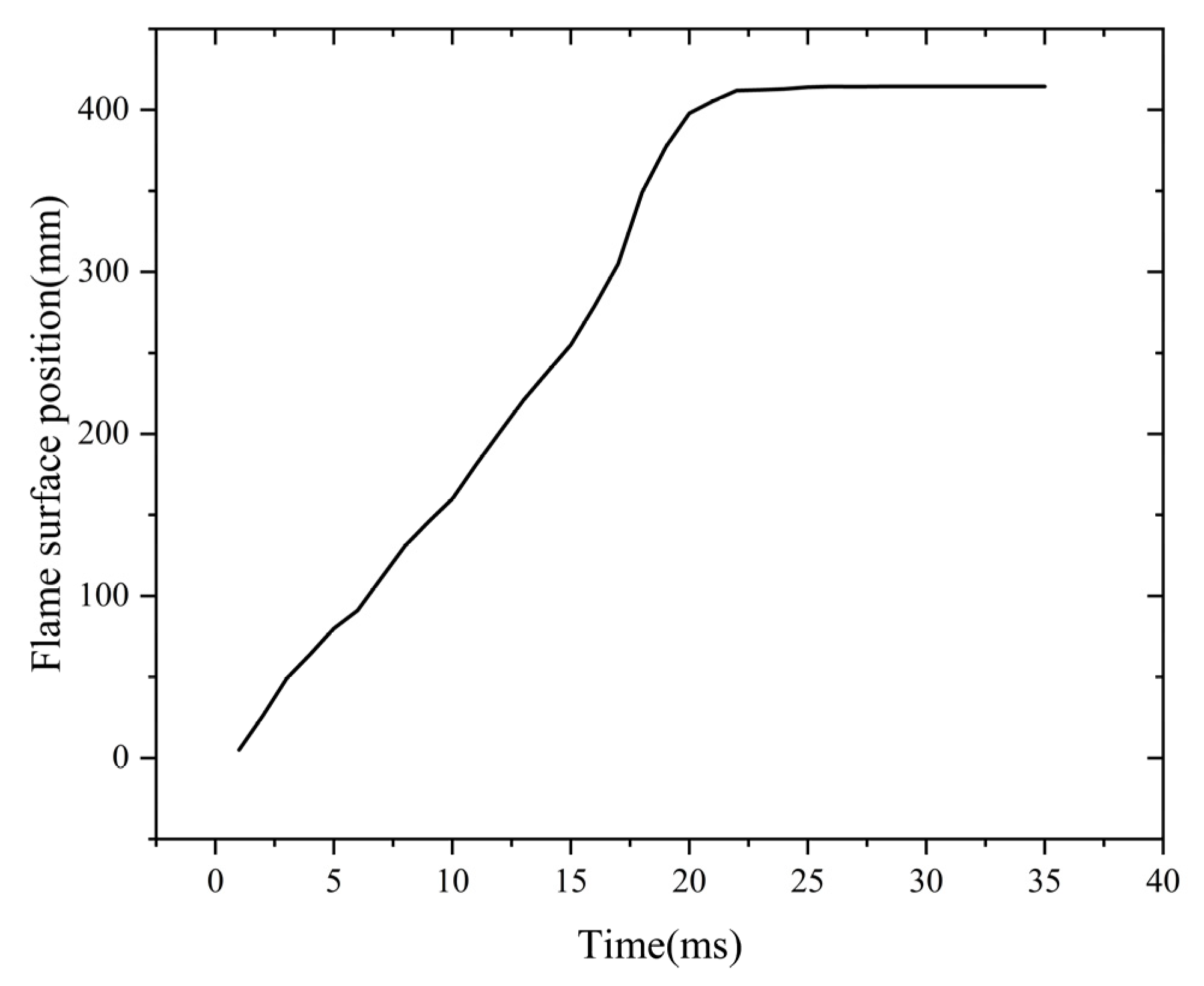Figure 8 illustrates the variation in the flame front position throughout the propagation and quenching stages. Figure 8 shows the dynamic evolution of the flame front position over time.

The data points in Figure 8 show that after ignition, the flame propagates within the flame arrester system. At t = 21 ms, the flame reaches the flame-arresting core. This is the start of the quenching process. Then, the flame advances a certain distance through the core. At t = 26 ms, the flame reaches its maximum advancement within the core. This maximum distance is defined as the quenching length of the flame arrester. After t = 26 ms, the propagation distance remains unchanged. This means the flame has been quenched successfully.

5.4. Parametric Studies

The effect of parameters such as porosity, flame arrester core thickness, inlet flame velocity, and flame arrester length on the quenching length is discussed as follows.

(1)

Analysis of the influence of porosity

Flame quenching simulations were carried out on methane–air pipeline flame arresters. The diameter of the arresters is 60 mm. The porosity gradients range from 0.2 to 0.9, and the pipe length is 400 mm. Figure 9 illustrates the change in quenching length related to porosity at different flame velocities.

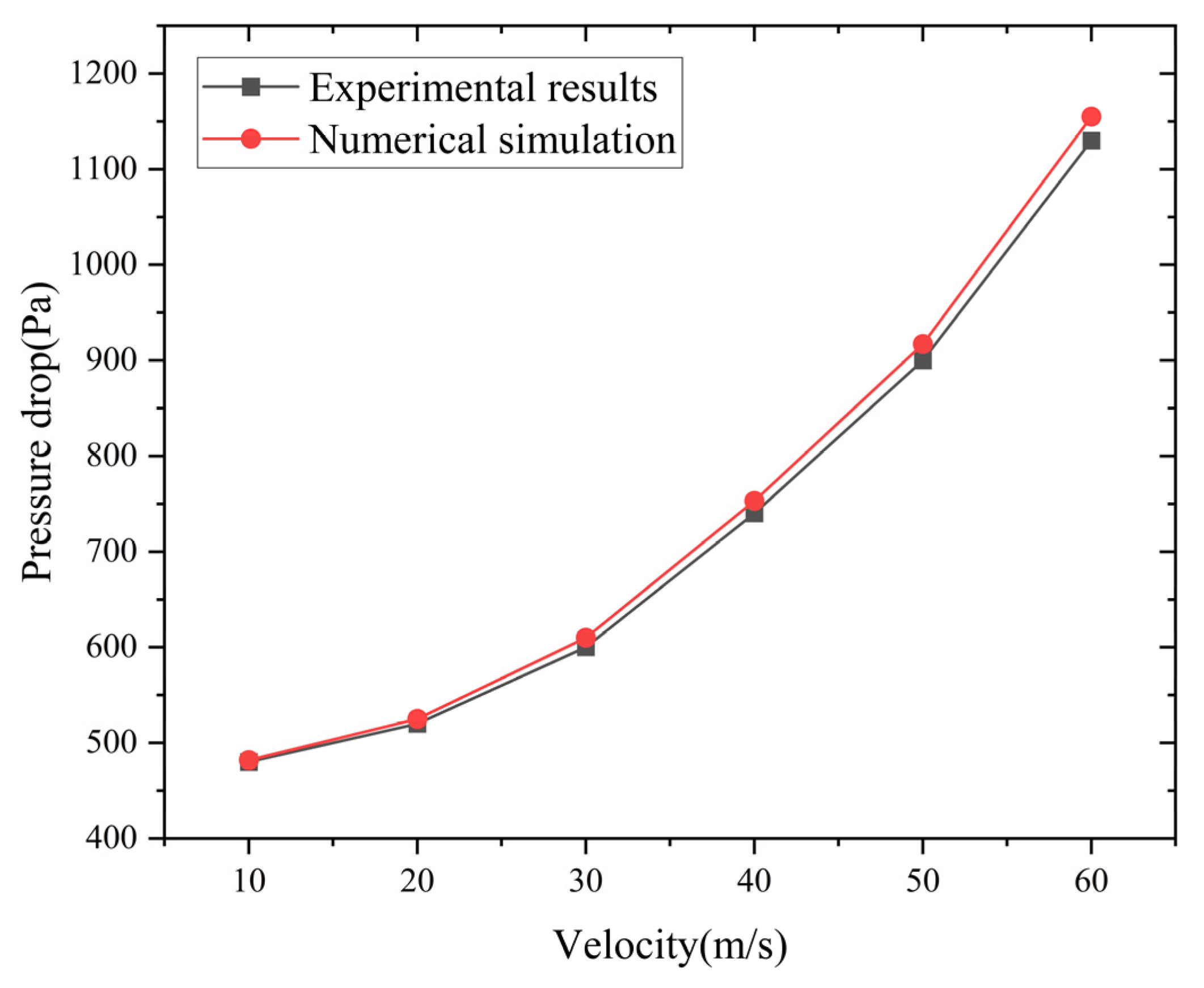
The numerical results show that there is a positive correlation between the porosity increment and maximum flame propagation distance within the arrester matrix. This relationship shows that when the porosity decreases from 0.9 to 0.2, the flame-quenching efficiency improves significantly. In low-porosity configurations, better suppression ability is achieved because of stronger thermal dissipation and flow resistance effects. However, as the porosity decreases, the pressure drop across the flame arrester will increase. Thus, in engineering design, the porosity must be precisely regulated within an appropriate and optimized range to ensure both effective flame-arresting performance and acceptable pressure drop levels.

(2)

Analysis of the influence of the flame arrester core thickness

Flame arrester cores with thicknesses of 80, 100, 120, 140, 160, and 180 mm were investigated. Figure 10 demonstrates the thickness-dependent quenching characteristics under varying flame velocities. The simulated data show an exponential decay pattern of quenching length with increasing core thickness. These findings confirm that the flame arrester core thickness effectively enhances the flame-quenching efficiency in methane–air mixtures. It does so by extending the heat dissipation paths and prolonging the gas residence time.

(3)

Analysis of the influence of the inlet flame velocity

Flame arresters with inlet velocities from 10 to 80 m/s were analyzed. Figure 11 shows the quenching length dependence on inlet velocity across varied arrester configurations. The simulation results indicate an exponential growth pattern of quenching length with increasing inlet velocity. This relationship between inlet flame velocity and quenching length shows that reducing the inlet flow speed effectively suppresses methane–air flame propagation.

(4)

Analysis of the influence of the flame arrester length

The flame arrester length’s effects on the quenching characteristics are presented in Figure 12. The simulated data show a positive relationship between the arrester length and quenching length. Shorter arresters have better flame suppression efficiency. Theoretically, a longer flame arrester allows for more sufficient heat exchange. However, if the length of the flame arrester is too long, the flow resistance of the flame arrester to the gas will increase. This increase in flow resistance leads to a larger quenching length.

5.5. Quenching Length Prediction Model Based on Response Surface Method

The single-factor numerical simulation results were studied. The analysis revealed four key influencing factors for flame quenching length. These factors are porosity (A), flame arrester core thickness (B), inlet flame velocity (C), and flame arrester length (D). A Box–Behnken experimental design was adopted to evaluate the effects of these factors. In this study, the quenching length was measured as the response variable. A design with four factors and three levels was carried out. It follows the principles of the Box–Behnken central composite design. The rules of the test design are detailed in

Table 5. Experimental factors and corresponding levels.

Factor	Factor Name	Unit of Factor	Low Level	High Level
A	Porosity	—	0.2	0.9
B	Flame arrester core thickness	mm	80	180
C	Inlet flame velocity	m/s	10	80
D	Length of the flame arrester	mm	40	100

. The selected factor levels were determined based on numerical simulation trends. The experimental schemes and corresponding simulation results are shown in

Table 6. Experimental scheme and results of Box–Behnken.

Number	Factor 1: A	Factor 2: B (mm)	Factor 3: C (m/s)	Factor 4: D (mm)	Response Value (mm)
1	0.2	80	45	70	2.68
2	0.9	80	45	70	3.6
3	0.2	180	45	70	1.97
4	0.9	180	45	70	3
5	0.55	130	10	40	2.25
6	0.55	130	80	40	2.65
7	0.55	130	10	100	2.51
8	0.55	130	80	100	3.2
9	0.2	130	45	40	2.26
10	0.9	130	45	40	3.22
11	0.2	130	45	100	2.65
12	0.9	130	45	100	3.64
13	0.55	80	10	70	2.55
14	0.55	180	10	70	1.95
15	0.55	80	80	70	3.15
16	0.55	180	80	70	2.44
17	0.2	130	10	70	2.2
18	0.9	130	10	70	2.95
19	0.2	130	80	70	2.52
20	0.9	130	80	70	3.72
21	0.55	80	45	40	2.75
22	0.55	180	45	40	2.08
23	0.55	80	45	100	3.14
24	0.55	180	45	100	2.5
25	0.55	130	45	70	2.8
26	0.55	130	45	70	2.8
27	0.55	130	45	70	2.8
28	0.55	130	45	70	2.801
29	0.55	130	45	70	2.8

.

Based on 29 experimental response values in Table 6, a regression model (Equation (14)) was created. This regression model is a quadratic regression equation that includes linear terms, interaction terms, and quadratic terms.

$$\begin{array}{l}Y=+1.61647-0.789102A+0.009203B+0.008860C+0.006699D\\ +0.001571AB+0.009184AC+0.000714AD-0.000016BC+0.000005BD\\ +0.000069CD+1.37673A^2-0.000063B^2-0.000099C^2-0.000029D^2\end{array}$$

(14)

where Y is the quenching length, A is the porosity, B is the flame arrester core thickness, C is the inlet flame velocity, and D is the length of the flame arrester.

The analysis of variance of the regression model is shown in

Table 7. Parameter optimization analysis of variance.

Source of Variance	Sum of Squares	d.f.	Mean Square	F-Value	p-Value	Level
Model	6.13	14	0.4378	7.661 × 106	<0.0001	Significant
A	2.85	1	2.85	4.991 × 107	<0.0001	Significant
B	1.29	1	1.29	2.252 × 105	<0.0001	Significant
C	0.8911	1	0.8911	1.559 × 105	<0.0001	Significant
D	0.4921	1	0.4921	8.611 × 105	<0.0001	Significant
AB	0.0030	1	0.0030	52,937.5	<0.0001	Significant
AC	0.0506	1	0.0506	8.859 × 105	<0.0001	Significant
AD	0.0002	1	0.0002	3937.5	<0.0001	Significant
BC	0.0030	1	0.0030	52,937.5	<0.0001	Significant
BD	0.0002	1	0.0002	3937.5	<0.0001	Significant
CD	0.0210	1	0.0210	3.679 × 105	<0.0001	Significant
A2	0.1845	1	0.1845	5.35 × 105	<0.0001	Significant
B2	0.1586	1	0.1586	2.775 × 105	<0.0001	Significant
C2	0.0955	1	0.0955	1.672 × 105	<0.0001	Significant
D2	0.0045	1	0.0045	78,814.99	<0.0001	Significant
Residual	8.0 × 10−7	14	5.714 × 10−8	—	—	—
Lack of fit	0.0001	10	0.00001	0.00001	0.991	No significant
Pure error	8.0 × 10−7	4	2.0 × 10−7	—	—	—
Sum total	6.13	28	—	—	—	—

.

Based on the statistical analysis presented in Table 7, the model shows an extremely high significance level. The F-value is 7.661 × 10⁶ and the p-value is less than 0.0001, which confirms that the regression equation is highly reliable. The lack-of-fit F-value is 0.00001 and the p-value is 0.9999 (>0.05). The lack of fit is insignificant. The model’s residual error is mainly due to random variation rather than systematic error. The response values predicted by the quadratic regression equation show no significant deviation from the measured values.

Based on the F-values of individual factors, A, B, C, D and their combinations are found to have a significant impact on the quenching length. These combinations include AB, AC, AD, BC, BD, CD as well as A², B², C², D².

The F-value indicates the relative influence of each factor on the quenching length. Higher F-values mean stronger effects. The results of the tests validate the significance order as follows: porosity (A) > flame arrester length (D) > flame arrester core thickness (B) > inlet flame velocity (C). This order reveals that porosity is the most dominant factor affecting the quenching length. The flame arrester length ranks second. The flame arrester core thickness comes third. The inlet flame velocity has the weakest effect.

As shown in

Table 8. Correlation parameter values.

Parameter Name	Parameter Value
Std. Dev	0.0002
Mean	3.00
C.V.%	0.0080
R2	0.9999
Adjusted R2	0.9999
Predicted R2	0.9999
Adeq Precision	9132.1292

, the regression model has a high degree of goodness of fit. The R² is 0.9999 and adjusted R² is 0.9999, both of which are close to 1.0. The regression model can explain the majority of the changes in quenching length. The Adequate Precision (Adeq Precision) value is 9132.1292. This value is much larger than the threshold of 4. The regression model provides a strong signal-to-noise ratio for reliable predictions. Adeq Precision assesses the proportion of the predicted response signal relative to the background noise. When the value exceeds 4, it indicates that the model has strong predictive accuracy. These statistical indicators are consistent with the results in Table 7. The high F-value, low p-value, and insignificant lack-of-fit term all confirm that the regression model is both significant and reliable for predicting quenching length.

6. Conclusions

(1)

Based on the fundamental theories of flame propagation and quenching, a numerical analysis model for a pipeline flame arrester is constructed. The model combines governing equations, the standard k-ε turbulence model, combustion model, and porous media model. The model is solved by using Ansys Workbench.

(2)

The characteristics of flame propagation and quenching are revealed by analyzing the flow field of the flame arrester. The distributions of flame temperature and chemical reaction rate at different time points are obtained. The temperature criterion for flame quenching in numerical simulations is proposed.

(3)

The effects of flame arrester porosity, core thickness, inlet flame velocity, and flame arrester length on the quenching length are investigated. The results indicate that the quenching length increases with porosity and inlet flame velocity, and decreases with core thickness. The quenching length becomes longer as the flame arrester length increases.

(4)

The response surface method is employed to predict the quenching length. A predictive equation for quenching length under different factor combinations is established. The equation has a high degree of goodness of fit. The influence of each factor on the quenching length follows the following order: porosity > flame arrester length > flame arrester core thickness > inlet flame velocity.

(5)

This work provides a robust numerical foundation for flame arrester design, bridging theoretical insights with engineering applications. Future efforts should focus on scalability to real-world industrial systems and dynamic flame arrester interactions under transient conditions.

References

1. Nie, Z.; Gao, W.; Jiang, H.; Zhao, F. Quenching characteristics and mechanism of hydrogen-air mixtures by corrugated plate flame arrester under inert conditions. Fuel 2024, 362, 130822. [Google Scholar] [CrossRef]
2. Wang, L.Q.; Ma, H.H.; Shen, Z.W.; Chen, D.G. Flame quenching by crimped ribbon flame arrestor: A brief review. Process Saf. Prog. 2019, 38, 27–41. [Google Scholar] [CrossRef]
3. Thomas, G.; Oakley, G.; Bambrey, R. Fundamental studies of explosion arrester mitigation mechanisms. Process Saf. Environ. Prot. 2020, 137, 15–33. [Google Scholar] [CrossRef]
4. Bao, L.; Wang, P.; Dang, W.; Kuang, C.; Yu, A. Experimental study on detonation flame penetrating through flame arrester. J. Loss Prev. Process Ind. 2021, 72, 104529. [Google Scholar] [CrossRef]
5. Cao, X.; Zhou, X.; Zhou, J.; Wang, Z.; Li, A.; Bi, S.; Ding, Z. Study on the resistance characteristics of corrugated flame arrester for hydrogen explosion. Clean Energy 2025, 9, zkae124. [Google Scholar] [CrossRef]
6. Farah, H.A. Numerical Study of Detonation Flame Arrestor Performance and Detonation Interaction with the Arrestor Element; The University of Texas at Arlington: Arlington, TX, USA, 2019. [Google Scholar]
7. Fonseca, E.M.M.; de Melo, F.J.M.Q.; Oliveira, C.A.M. The thermal and mechanical behaviour of structural steel piping systems. Int. J. Press. Vessel. Pip. 2005, 82, 145–153. [Google Scholar] [CrossRef]
8. Zong, S.; Liu, K.; Qiu, W.; Gao, Z.; Wang, J. Numerical and Experimental Analysis of Fire Resistance for Bulkhead and Deck Structures of Ships and Offshore Installations. J. Mar. Sci. Eng. 2023, 11, 1200. [Google Scholar] [CrossRef]
9. Yue, J.; Long, W.; Liu, H.; Guo, S. A novel detonation arrester containing a large disk with long triangular slits: Design and numerical simulation. Process Saf. Prog. 2021, 40, e12176. [Google Scholar] [CrossRef]
10. Liu, D.; Sun, S.; Wang, L. Numerical Simulation of the Propagation of Premixed Gas in a Pipe Flame Arrestor. In Proceedings of the 2023 2nd International Conference on Green Energy and Power Systems (ICGEPS 2023), Changsha, China, 6–8 January 2023; IOP Publishing: Bristol, UK, 2023. [Google Scholar]
11. Farah, H.A.; Lu, F.K.; Griffin, J.L. Numerical Study of the Pressure Drop in a Flame Arrestor Using a Porous Media Model. In ASME International Mechanical Engineering Congress and Exposition; American Society of Mechanical Engineers: New York, NY, USA, 2020. [Google Scholar]
12. Jovanovic, J. The Statistical Dynamics of Turbulence; Springer Science & Business Media: Berlin/Heidelberg, Germany, 2013. [Google Scholar]
13. da Silva, C.V.; Deon, D.L.; Centeno, F.R.; França, F.H.R.; Pereira, F.M. Assessment of combustion models for numerical simulations of a turbulent non-premixed natural gas flame inside a cylindrical chamber. Combust. Sci. Technol. 2018, 190, 1528–1556. [Google Scholar] [CrossRef]
14. Xinglong, C.; Lixing, Z.; Jian, Z. Numerical simulation of methane-air turbulent jet flame using a new second-order moment model. Acta Mech. Sin. 2000, 16, 41–47. [Google Scholar] [CrossRef]
15. Krishna, Y.; Mahuthannan, A.M.; Luo, X.; Lacoste, D.A.; Magnotti, G. High-speed filtered Rayleigh scattering thermometry in premixed flames through narrow channels. Combust. Flame 2021, 225, 329–339. [Google Scholar] [CrossRef]
16. Cui, J.K. Numerical Study on Quenching Characteristics of Premixed Flame in Crimped Ribbon Flame Arrester Structural Element; East China University of Science and Technology: Shanghai, China, 2020. [Google Scholar]
17. Adler, J.; Spalding, D.B. One-dimensional laminar flame propagation with an enthalpy gradient. Proc. R. Soc. London. Ser. A. Math. Phys. Sci. 1961, 261, 53–78. [Google Scholar]
18. Hu, C.M. The Study of Premixed Flame Propagating and Quenching in Narrow Channel; Dalian University of Technology: Dalian, China, 2006. [Google Scholar]
19. Song, Z.B. Research on the Propagation Mechanism and Quenching Conditions of Premixed Flames in Slits; Dalian University of Technology: Dalian, China, 2005. [Google Scholar]
20. Shi, D.Y. Study on Fire Resistance Characteristics of Honeycomb Fire Retarder with Light Hydrocarbon Mixed Gas; Xi’an Shiyou University: Xi’an, China, 2019. [Google Scholar]
Figure 1. A sketch of the pipeline flame arrester: (a) structure parameters; (b) the microchannels.
Processes 13 00847 g001
Figure 2. Internal flow field analysis model of pipeline flame arrester.
Processes 13 00847 g002
Figure 3. Grid diagram.
Processes 13 00847 g003
Figure 4. Temperature variation with mesh size.
Processes 13 00847 g004
Figure 5. Numerical simulation and experimental results were compared.
Processes 13 00847 g005
Figure 6. Flame distribution in the pipeline at different times.
Processes 13 00847 g006
Figure 7. Change in chemical reaction rate in fire-retarding system at different times.
Processes 13 00847 g007
Figure 8. Flame surface position curve with time.
Processes 13 00847 g008
Figure 9. Effect of porosity on quenching length at different flame velocities.
Processes 13 00847 g009
Figure 10. Influence of core thickness ratio on quenching length at different flame speeds.
Processes 13 00847 g010
Figure 11. Influence of inlet flame speed on quenching length.
Processes 13 00847 g011
Figure 12. Influence of flame arrester length on quenching length.
Processes 13 00847 g012