Abstract
In modern process industries, precise process modeling plays a vital role in intelligent manufacturing. Nevertheless, both mechanistic and data-driven modeling methods have their own limitations. To address the shortcomings of these two modeling methods, we propose a neural network model based on process mechanism knowledge, aiming to enhance the prediction accuracy and interpretability of the model. The basic structure of this neural network consists of gated recurrent units and an attention mechanism. According to the different properties of the variables to be predicted, we propose an improved neural network with a distributed structure and residual connections, which enhances the interpretability of the neural network model. We use the proposed model to conduct dynamic modeling of a benzene–toluene distillation column. The mean squared error of the trained model is 0.0015, and the error is reduced by 77.2% compared with the pure RNN-based model. To verify the prediction ability of the proposed predictive model beyond the known dataset, we apply it to the predictive control of the distillation column. In two tests, it achieves results far superior to those of the PID control.
1. Introduction
With the advent of Industry 4.0, the process industry has an ever-growing and urgent demand for digital twins and smart manufacturing. Aspects such as product quality monitoring, process control, fault diagnosis, and process data soft sensing are directly related to the profitability of plants, all of which require analysis and modeling of the processes. Pallavicini et al. [1] have constructed a digital twin model of a biogas purification absorption unit through an approach that involves experimental data-aided mechanistic modeling. Utilizing this model, they have obtained a substantial amount of reliable data for the evaluation and analysis of the unit’s performance. This method has ensured the quantity and accuracy of the data while simultaneously reducing costs and enhancing the speed of analysis. Min et al. [2] have proposed a digital twin framework for the optimization of petrochemical production control based on the industrial Internet of Things and machine learning. They have implemented and evaluated this digital twin framework and methods in a catalytic cracking unit of a petrochemical plant. The results have demonstrated the effectiveness and value of the framework and methods in optimizing production control, leading to a reduction in production costs and an increase in production efficiency.
The classical solution involves constructing simulation models based on process mechanisms using equations grounded in physical knowledge. Mechanistic models can be distinguished based on whether they incorporate a time parameter, dividing them into steady-state models and dynamic models. Steady-state models are commonly utilized in the design and optimization of industrial processes, characterizing a stable point of the system. To predict future process data, however, all extensive quantities in the model equations must be associated with the time variable. Dynamic models constructed through such equations are more aligned with the actual industrial processes and can be effectively applied in scenarios such as product quality monitoring and process control. Tanaka et al. [3] have performed steady-state local linearization on a multistage countercurrent extraction process. They characterized the relationship between metal ions and independent operational variables using total differential equations at each stage, and they verified the reliability of this model. The influence of parameters on the process can be visually represented through charts obtained from this model, providing a theoretical foundation for dynamic modeling. Zhang et al. [4] have employed the most classical mechanistic modeling approach to conduct steady-state and dynamic modeling of an ammonia synthesis reactor and the entire process. Based on this, they have investigated control strategies for the entire process. The optimal control strategy obtained can guide plants in reducing costs and increasing efficiency, exemplifying the value and significance of mechanistic modeling.
However, due to the uncertainties inherent in chemical processes, such as the decrease in the catalytic activity of catalysts, pipeline blockages, equipment corrosion, and changes in production procedures, mechanistic models are challenging to apply over an extended period without adjustments to all units. Furthermore, the construction of mechanistic models requires complex model equations, and the modeling process itself demands considerable labor. For large-scale industrial processes, the resource expenditure is substantial, particularly when changes in the production process occur, leading to model mispatch. In such instances, remodeling becomes necessary, which is an onerous task. This results in the limitations of the application of mechanistic models in actual industrial settings.
In recent years, data-driven model construction methods have been increasingly becoming the mainstream approach in research and application. On one hand, thanks to comprehensive industrial big data systems, the collection and storage of industrial process data have become quite straightforward; on the other hand, due to the rapid development of computer hardware computing power and the widespread application of artificial intelligence neural network algorithms, the rapid and efficient analysis of large-scale data has become feasible. Gao et al. [5] proposed a hybrid modeling strategy for the gas-phase catalytic coupling synthesis of dimethyl oxalate from carbon monoxide, which integrates process mechanism and data-driven methods, and its effectiveness has been verified. Savage et al. [6] tackled the inefficiency issues of traditional surrogate modeling and superstructure optimization techniques in dealing with complex process flows such as utility and refrigeration systems, by proposing an inherited data-driven modeling and optimization framework, which has been rigorously validated for its accuracy as well as its advantages in solution efficiency and flexibility. Chen et al. [7], in response to the complex chemical kinetic processes represented by the enzymatic biodiesel production system, have developed a modeling framework that combines prior physical knowledge with data-driven approaches, and have verified its accuracy and reliability. Alauddin et al. [8] have proposed a Process Dynamics-Guided Neural Network (PDNN) model to enhance the model’s generalization capability, which maintains superior performance in sparse and low-quality data environments.
In addition, numerous scholars have utilized neural networks to construct surrogate models for dynamic processes and have applied them within model predictive controllers, achieving favorable outcomes. Sharma et al. [9] investigated the tert-amyl methyl ether reactive distillation column and compared three control strategies: PID, Model Predictive Control (MPC), and Neural Network Model Predictive Control (NMPC). The study found that the NMPC exhibited the best performance. Li et al. [10], addressing the control issues of an intensified continuous reactor, proposed and implemented two nonlinear model predictive control algorithms based on neural networks. Through simulation, it was demonstrated that the algorithm with local linearization performed better. Jian et al. [11] introduced a multi-time-scale process modeling method based on Multi-Time-Scale Recurrent Neural Networks (MTRNNs) and validated the method’s effectiveness in multi-time-scale modeling through a Continuous Stirred Tank Reactor (CSTR). Rebello et al. [12] have formulated a set of guidelines for the identification of machine learning models in diverse applications within process systems engineering, which are commonly utilized for simulation or predictive purposes. They demonstrated that relying solely on test performance without considering the specific application context can be misleading. Xu et al. [13] have introduced a nonlinear identification method based on a Self-Adaptive Mechanism Regulated Long Short-Term Memory (SA-MRLSTM) network, which exhibits robustness and commendable generalization capabilities.
However, compared to classical mechanistic models, data-driven modeling methods suffer from a lack of interpretability, which makes it difficult for industrial personnel to place full trust in data-based model construction approaches. As a result, data-driven models face challenges in widespread application in actual industrial facilities. Many researchers have made attempts to fix this issue. Timur et al. [14] have explored various methods of integrating machine learning with process mechanisms and tested different models in a case study on multiphase flow estimation in petroleum production systems. Sun et al. [15] have proposed a comprehensive state-space description system and the corresponding hybrid first-principles/machine learning modeling framework, providing a theoretical foundation for intelligent manufacturing solutions in the process industry. Li et al. [16] have developed a Light Attention–Convolution–Gate Recurrent Unit (LACG) architecture to render data-driven dynamic chemical process models interpretable and have validated its efficacy. The model parameters of the LACG afford the observation of more detailed insights regarding the interactions between variables.
At present, research that combines model-driven and data-driven approaches for dynamic modeling, which holds higher application value, is quite rare. Generally, there are three methods to achieve the integration of mechanistic models and data-driven approaches [17]: The first method involves incorporating process mechanism knowledge when constructing the dataset, imposing physical constraints on input data, using parameters obtained from mechanistic models as inputs during model construction, and adding data generated by the mechanistic model to the dataset as training and test sets. The second method entails adding process mechanism constraints within the hidden layers of deep neural networks, such as modifying the hidden layer structure, incorporating additional intermediate output variables based on the mechanistic model, and altering the construction of the loss function. The third method involves imposing process mechanism constraints at the output stage, making judgments and selections of output parameters that align with chemical engineering knowledge through the experience and expertise of process engineers or the application experience of actual equipment. In our research, we focus on the first method, employing the results of mechanistic models to expand the dynamic range of the model, enhancing the generalization capability of data-driven models, and ensuring interpretability in the structure of input–output relationships.
Therefore, we have conducted research in this area and attempted to apply it to the predictive control of distillation systems. As one of the most typical unit operations in chemical engineering, distillation systems involve complex processes of mass transfer, momentum transfer, and heat transfer. The operational efficiency of distillation systems is intimately associated with the profitability of the production process. Specifically, the utility consumption of condensers and heaters affects the secondary costs of production, while the product quality, which determines the product’s market value, is a direct reflection of whether the product meets standards. This is the reason why distillation systems have long been a focus of attention. In this paper, we investigate a benzene–toluene distillation column, using a process mechanism to analyze the distillation system. Based on this analysis, we utilize a neural network with a targeted architecture to construct a predictive model for the distillation column, which is capable of forecasting the operational state of the distillation column over a certain period in the future. By constructing a surrogate model for the dynamic process of the distillation system, we can effectively predict the operational state of the system, thereby reducing energy consumption and increasing profitability.
The remainder of this paper is organized as follows: Section 2 is the Methodology section, where we first introduce the fundamental structures of neural networks such as recurrent neural networks and attention mechanisms. Subsequently, we discuss the improvement strategies for neural networks based on process mechanisms, and a brief introduction of the accompanying model predictive controller is also provided in this section. Section 3 is the Application and Discussion section, where we demonstrate the effectiveness of the proposed model in constructing predictive models for distillation processes and apply the predictive model to predictive control tasks. The conclusions of this study are summarized in Section 4.
2. Methodology
2.1. Recurrent Neural Network (RNN)
Chemical process data belong to time series data, which can be characterized as continuous data in the time domain and exhibit a certain degree of autocorrelation. Consequently, the data can reflect the state of the process system as it changes over time, and there is a relationship between the data of the subsequent time step and that of the preceding time step. In chemical processes, Recurrent Neural Networks (RNNs) are naturally suited for handling such systems and have demonstrated favorable performance. For instance, the Gated Recurrent Unit (GRU) model is capable of fully exploiting the dynamic and nonlinear relationships between input and output variables and has shown good performance in applications. This model primarily consists of a reset gate and an update gate. The update gate is used to compute the update rate , calculated as follows:
where xt is the input of the current time step, ht−1 is the hidden state of the last time unit, Wz is the input weights, and Uz is the hidden state weights. The update gate helps the model to decide how much information from the previous time step and the current time step needs to be passed on.
Similarly, the reset gate can be represented as the following formula:
The reset gate determines how much past information needs to be forgotten by the memory units.
The hidden state of the current time step can be computed by the following:
Candidate variable can be written as follows:
where is the input weights, is the hidden state weights, and is the Hadamard product.
2.2. Attention Mechanism
The attention mechanism was initially proposed by researchers at Google [18] to enhance the recognition efficiency of seq2seq models when performing NLP tasks. The attention mechanism assigns weights to each input variable. The method for calculating the attention weights is as follows:
where stands for query, which is the query vector; represents key, which is the key vector; and denotes value, which is the vector of input parameter values. The vector produced by the aforementioned equation has been processed by the attention mechanism. The allocation ratio of attention weights can be visualized using a heatmap, as illustrated in Figure 1:
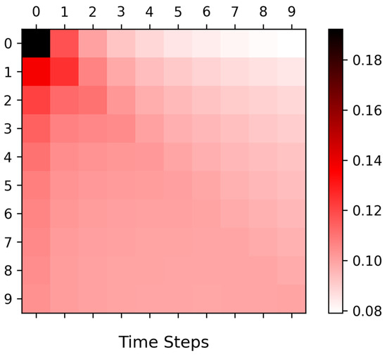
Figure 1.
Heatmap of attention weights.
In our work, the method employed is a special case of the attention mechanism known as self-attention. The characteristic of self-attention lies in the fact that the matrices used to compute the vectors , , and are the same matrix. This allows us to process the various input parameters to obtain attention in the feature dimension. The calculation method is as follows:
2.3. Neural Network Architecture
In this study, a neural network sub-model is constructed using Gated Recurrent Units (GRUs) and Attention Mechanism. The structure of this sub-model is depicted in Figure 2. Time series data must first undergo data preprocessing, which will be introduced as follows, and then these preprocessed data are fed into the self-attention layer for the extraction of latent relationships between variables. After the allocation of attention weights, the processed variables are passed through the GRU layer for feature extraction along the temporal dimension. Following the processing by the GRU layer, the time series data are compressed into a single context vector, which is believed to encapsulate all the information of the current time step. The context vector obtained from the previous step is then fed into a Feedforward Neural Network (FNN) composed of three layers of Multilayer Perceptions (MLPs) for computation, and the final results are obtained through the output layer. The activation function between layers is the Exponential Linear Unit (ELU) function. The ELU function is a variant of the Rectified Linear Unit (RELU) function, which is smoother at zero, facilitating gradient computation during backpropagation.
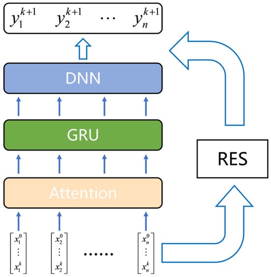
Figure 2.
Structure of sub-model.
Repeated experiments have shown that a more complex network structure, a larger network scale, and an increased number of network layers fail to improve the predictive performance of neural networks. Conversely, these factors can lead to more difficult convergence of the neural network, resulting in an inability to improve model accuracy and a decline in predictive efficacy. Therefore, we do not optimize the structure of the sub-models. In the subsequent section, the focus is on the utilization of these sub-models to construct a complete predictive model.
2.4. Dynamic Process Mechanism Model
In chemical engineering processes, there are numerous unit operations, each with its distinct internal structure. To describe these different unit operations, various model equations are required. However, regardless of the type of unit operation model, their dynamic models can be generalized as a system of differential equations and algebraic equations, which can be represented by the following equation set:
where and denote all the variables within the process; represents time; is the disturbance variable, expressed as a time-variant function.
However, there are numerous unknown variables in the model equations. A significant number of these variables cannot be directly measured by sensors, such as enthalpy, fugacity, and other thermodynamic parameters, and equipment parameters like heat transfer coefficients, separation efficiency, and pipe friction factors. Consequently, when modeling an actual plant, it is challenging to reduce model errors through parameter calibration, leading to certain dilemmas in the application of mechanistic models. Data-driven modeling methods can utilize specific measurement data from the process for analysis, thereby compensating for the deficiencies of mechanistic models in this regard.
For the purpose of applying dynamic models in predictive control, it is necessary to first deliberate upon the classification of variables. From the perspective of interactions between operators and the system, as well as between the environment and the system, variables can be categorized into four distinct types: state variables, control variables, environmental variables, and equipment parameters.
State variables represent the physical quantities used to characterize the current motion state of a system during the occurrence of transfer phenomena within the system. These variables are influenced by changes in external conditions and by human manipulation, and they are essential for calculating the system’s state at the subsequent moment. Examples include the pressure inside a distillation column, the temperature within a reactor, and the flow rate on a particular side of a heat exchanger.
Control variables represent the variables directly influenced by human operational actions, and the variation of these variables can impact the dynamic state of the system. Typical control variables include the opening of a throttle valve, the rotational speed of a compressor, and the power supplied to an electrolytic cell.
The distinction between environmental variables and control variables lies in the fact that environmental variables are not subject to human control and represent external influencing factors. Environmental variables can also impact the dynamics of the system. For instance, environmental variables may include the pressure at the boundary of the system, the content of impurities in the feedstock, and the ambient temperature around the industrial site.
The meaning of equipment parameters is self-evident; these variables are characterized by their independence from human operation and external environmental changes. They remain constant throughout the system’s dynamics. However, these variables are essential inputs for the development of mechanistic models. Examples include the heat transfer area and coefficient of a heat exchanger, the flow capacity of a valve, and the volume of a storage tank.
Upon substituting the aforementioned variables into the model equations and reorganizing them, the general set of equations for dynamic models used in predictive control can be represented as follows:
Owing to the requirement for numerical computations, the aforementioned continuous representation is subjected to discretization. Concurrently, in order to enable iterative calculations, it is necessary to convert the representation into an iterative form:
Ultimately, a formulation has been developed that can be represented as an input-to-output relationship and is amenable to direct iterative computation. By using the receding horizon method, it is possible to calculate the values of variables at future time instances, achieving the effect of over-horizon prediction. Applying this formulation to the input–output structure of machine learning models enables the establishment of a discretized data-driven process dynamic model.
However, it can be observed that within the model equations, there is a requirement for solving algebraic equation sets as well as integrating differential equation sets to determine the variables. In conventional methods, it is typical to first solve the algebraic equations followed by the integration process, resulting in some variables being derived from algebraic equations, while others are obtained through integration. The process of solving mechanistic models and applying them to predictive tasks can be regarded as a forward problem, whereas the use of historical data to identify parameters within the model equations constitutes an inverse problem. Similarly, if we can train a neural network model that is equivalent to the inverse problem using numerical methods, then the forward propagation process of the neural network model is equivalent to solving the mechanistic model. Under this premise, the process of training data-driven models can be viewed as a process of fitting algebraic equations and ordinary differential equations (ODEs).
A combined form of multiple sub-models is proposed, embedding prior mechanistic model knowledge into the neural network model. By incorporating sub-models within the neural network, the equations used to solve for each variable are approximated, thereby replacing the solution process of the mechanistic model and enhancing the interpretability of the neural network model. These concepts will be further elaborated in the subsequent section.
2.5. Strategies for the Enhancement of Multivariate Prediction Networks
In practice, single recurrent neural networks face challenges in multivariate prediction. Thus, a distributed network architecture optimized for such tasks is employed. In the present work, the entire model is replaced with multiple sub-models, each tasked with predicting a single variable. At the output layer of the neural network, all variables to be predicted are aggregated into a single array to serve as the output of the prediction model. The efficacy of this distributed model will be compared and demonstrated in the application section, with the model architecture illustrated in Figure 3.
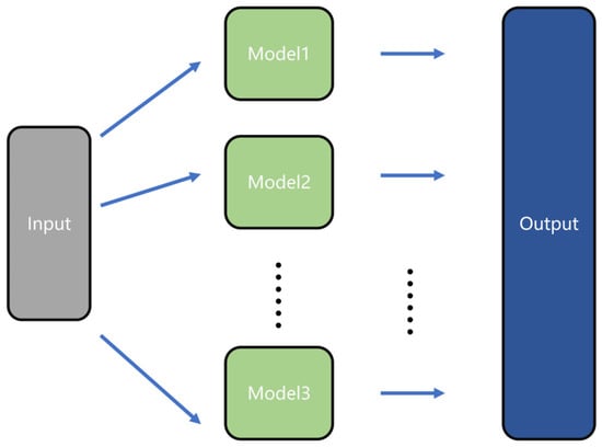
Figure 3.
Structure of distributed network.
Simultaneously, it is noted that for multivariate prediction in large-scale systems, the correlation between the variables to be predicted and the input variables is a consideration worth examining. In industrial processes, two-unit operations that are spatially distant may exhibit a time lag within the sampled time steps, such that the relationship between the variables of these two operations may not be captured. For instance, in a distillation sequence consisting of three distillation columns, an increase of 5 °C in the feed temperature may take several hours to propagate to the vapor phase outlet temperature of the last column in the sequence. However, the model does not sample forward for such an extended number of time steps during forward sampling. If machine learning models are directly applied to learn from the dataset without any preprocessing, such fundamentally uncorrelated variables might be mis-learned. To prevent this occurrence, a model mask is introduced at the beginning of the neural network model to enhance the precision of the prediction model and accelerate the convergence of the model.
The mask can be represented as a matrix of size input dimension × output dimension, denoting the connectivity relationship from inputs to outputs, where a value of 1 indicates connectivity and a value of 0 indicates disconnection. When combined with the proposed distributed network, the form of the model can be simply represented by the following equation:
By integrating the distributed network architecture with the model mask, it is possible to employ different sub-models for distinct variables and utilize different input variables for each sub-model, as illustrated in the figure. The advantage of this approach lies in the ability to decouple the prediction tasks for individual variables, and even to optimize the parameters of each sub-model separately, until a model with satisfactory precision is trained.
In the process of solving model equations, there are complex computational procedures. The model equations include tasks such as solving algebraic equations and integrating variables within differential equations. The conventional approach is to first handle the algebraic equations, obtaining results for some variables, and then conduct integration operations to determine the values of the other variables. From a modeling perspective, solving mechanism models for prediction tasks is considered a direct problem, while using historical data to determine the parameters in the model equations is considered an inverse problem.
If a neural network model equivalent to the inverse problem is trained using numerical methods, then the forward propagation process of this neural network model is equivalent to the solving process of the mechanism model. Based on this principle, the training process of data-driven models is actually a process of fitting algebraic equations and ordinary differential equations (ODEs).
To better harness the model’s performance, we adopt a combination of multiple sub-models, incorporating prior knowledge of mechanism models into the neural network model. By using the sub-models of the neural network to approximate the equations for solving various variables, we replace the complex solving process of the mechanism model and also enhance the interpretability of the neural network model.
Therefore, for the problem of solving ODEs, we have added residual connections to the network. The fundamental structure of the residual network can be described in the following form:
where represents the “optimal function” output by the residual network; represents the residual function within the residual network.
Residual networks were first proposed by researchers at Microsoft and applied to deep convolutional neural networks for image recognition [19]. Residual connections are capable of alleviating the difficulty of training and reducing the occurrence of overfitting.
Departing from conventional research, some scholars have explored the relationship between residual networks and ODEs/PDEs, providing a mathematical interpretation of residual networks based on differential equations, and proposing the feasibility of using residual networks for dynamic system modeling [20,21]. Indeed, by referencing Equations (9a) and (11), the residual network is also clearly similar in form to ODE, and this connection is easily discernible. By leveraging this relationship, units with residual connections can solve ODEs more efficiently. In other words, the model can more effectively predict variables that would originally need to be solved through integration in the model equations, which are various extensive quantities, such as heat, liquid holdup, etc.
In our research, sub-models with residual connections are used to predict variables that are solved using ODEs in the mechanism model, while the remaining variables are predicted using sub-models without residual connections. This approach is selectable for different variables.
Figure 4 illustrates the architecture of a neural network model for predictive control. The grey dashed lines in Figure 4 represent the input layer connections that are masked by the model mask. Sub-models have the option to include a residual connection module, and each sub-model can freely select the input variables it requires. Finally, the predictions from the sub-models are aggregated into a single output vector.
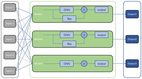
Figure 4.
Distributed network model within residual connections.
2.6. Data Acquisition, Dataset Compilation, and Data Preprocessing
Process systems are inherently continuous, both at the microscopic and macroscopic levels. However, when focusing on modeling, particularly when computational solutions are required, the model equations must be discretized in the temporal dimension to facilitate numerical solution methods. The discretization of time necessitates consideration of the corresponding time intervals that arise post-discretization. In the context of mechanistic modeling, this time interval refers to the integration time, whereas for process monitoring and subsequent process data analysis, it refers to the sampling interval during measurement. Different modeling approaches require different time intervals, and in practice, the sampling intervals may vary even for different variables. Therefore, it is essential to align the time scales to facilitate the modeling of input-to-output relationships. Moreover, the length of the time interval must be considered; an excessively long interval may result in data-driven models failing to capture sufficient information, leading to an inadequate approximation of the true process. Conversely, an overly short interval may cause unexpected overfitting due to the measurement noise inherent in the data. In our work, the integration time for the mechanistic model is set at 0.5 s, and the sampling interval for data-driven approaches is uniformly set at 5 s, a determination made through experimentation and constrained by computational speed.
Based on the established sampling rate, a time series dataset comprising 100 thousand data points was acquired and subjected to preprocessing. The min–max normalization method was employed to scale the data within the range of 0 to 1. The min–max normalization method can be described by the following expression:
Since it is necessary to compute the mean squared error for variables with different data dimensions, normalizing all variables to have the same data dimensionality renders the loss function and accuracy evaluation metrics more meaningful.
Subsequently, the dataset was partitioned into training, validation, and test sets according to a ratio of 7:1.5:1.5. The training set was utilized for the training of the neural network, while neither the validation nor the test set participated in the training process. The validation set served two purposes: first, to facilitate early stopping of the neural network training to prevent overfitting, and second, to optimize the hyperparameters of the neural network and the trainer. The test set was employed post neural network training to comprehensively evaluate the model’s fitting efficacy, including the assessment of the predictive performance for each predicted variable, as well as the distribution patterns of errors across the test set.
2.7. Model Predictive Control
To validate the efficacy of the proposed modeling methodology, we will apply the trained data-driven model to a predictive control task. A model predictive controller is utilized to manipulate the temperature and pressure within a distillation column, thereby controlling the concentration of the product.
The model predictive controller employed is the LMPC controller proposed by Wu et al. [22]. The objective of the MPC is to minimize the differences between the target trajectory and the predicted trajectory. The controller proposed by Wu et al. can be described as follows:
where denotes the model predictive trajectory; represents the control action trajectory; is the predictive model; Equation (13c) represents the error between the predicted trajectory and the actual trajectory. Wu et al. [23] have demonstrated that when the error of the predictive model is sufficiently small, the closed-loop stability of the controller can be guaranteed. For this reason, model accuracy is of great importance in the MPC. Equation (13d) represents the constraints on the control variables, and Equation (13e) denotes the equality and inequality constraints of the model.
In practical operations, the discrete form of the aforementioned is used, and the predictive model is described using discrete-time state-space equations. For the objective function, the explicit Euler method is employed for computation, which is formulated as follows:
where Equation (14a) represents the quadratic objective function; where is the prediction horizon; is the starting time of the prediction; is the predicted trajectory of the controlled variable; is the target trajectory; is the change in the manipulated variable; and are weight matrices. In the computation, at each sampling time, the controller establishes and solves the optimization problem based on historical data and current input data.
In addressing the optimization problem, it is necessary to repeatedly construct the prediction sequence. The method of constructing the prediction sequence is termed the moving horizon, and the specific procedure is delineated in Equation (15).
The method employs input variables at time step k to predict the state variables at time step k + 1 and utilizes the manipulated and environmental variables at time step k + 1 to predict the state variables at time step k + 2. This process is repeated in a cyclical manner to construct the prediction sequence . Following the construction of the prediction sequence, the objective function in Equation (14) can be optimized. The resulting optimization problem is a nonlinear optimization problem, which is typically solved iteratively using numerical methods. In this study, the Adam algorithm is employed for its resolution.
The Adam algorithm, known as Adaptive Moment Estimation, is a solution algorithm for nonlinear optimization problems, proposed by Kingma et al. [24] Derived from AdaGrad and RMSProp, Adam is an efficient stochastic optimization algorithm based on gradients. It was initially designed to address a variety of non-convex optimization problems in the field of machine learning, and in this study, it is applied to the solution of general nonlinear optimization problems. By solving the optimization problem constructed in Equation (14), the optimal control action trajectory and its corresponding predictive trajectory can be obtained. Once the solution is completed, only the initial several steps of the control action trajectory are implemented in the controlled system to achieve the optimal dynamic performance.
3. Results and Discussion
3.1. Introduction to Distillation Column
In the section pertaining to the mechanism model, the distillation system is modeled using equations of material balance, phase equilibrium, mole fraction summations, and heat balance (MESH).
Equation of material balance:
Equation of phase equilibrium:
Equation of mole fraction summations:
Equation of heat balance:
The system of interest comprises benzene and toluene, with the Peng–Robinson method utilized for phase equilibrium calculations. The distillation column operates at a pressure of 440 kPa, with a pressure drop of 13 kPa across the column. The column is configured with a total of 20 theoretical stages, and the feed is introduced at the 10th theoretical stage. The reflux ratio is 0.278. Steady-state flow rates are presented in Table 1.

Table 1.
Distillation process stream data.
As the neural network-based dynamic model in this study is designed for prediction control tasks, input and output variables are selected in accordance with the specific information of the control task.
Initially, it is essential to determine the overall control strategy based on the characteristics of the distillation column. Following the research by Konda et al. [25], after calculating the Control Degrees of Freedom (CDOF), it can be observed that for a benzene–toluene distillation column, which operates as a fully condensing reflux column, the control scheme depicted in Figure 5 is required. This scheme involves the control of four target variables, which are the liquid levels in the reflux drum and the column bottom, the column pressure, and the temperature of the sensitive tray. In Figure 5, the blue part represents the distillation section of the distillation column, the red part represents the stripping section of the distillation column, the green dotted line represents the control loop, and the label on the stream corresponds to the stream code in Table 1.
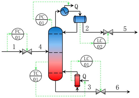
Figure 5.
Dynamic simulation flowsheet of distillation process.
In our study, the control strategy employs a hybrid MPC-PID control scheme. For the liquid levels in the flash drum and the column bottom, PID controllers are utilized to manipulate the withdrawal rates. For the column pressure and the temperature of the sensitive tray, an MPC controller is directly employed to manage the cooling and heating utilities at the column top and bottom, thereby controlling the column top pressure and the sensitive tray temperature. The comparison of this scheme with a PID-only control scheme clearly demonstrates the advantages of using predictive models, which will be elaborated upon in the discussion section.
In accordance with the requirements of the control task, there are five state variables required, which are the column top pressure, column bottom pressure, column top temperature, column bottom temperature, and the temperature of the sensitive tray. There are two environmental variables, namely, the feed temperature and feed flow rate. The control variables consist of the cooling capacity at the column top and the heating capacity at the column bottom.
Now that the variables involved in the model have been determined, the state variables, environmental variables, and operation variables at time k are taken as the input parameters of the model, and the state variables at time k + 1 are taken as the output parameters of the model. In this way, a machine learning model with an input dimension of 9 and an output dimension of 5 can be obtained.
After identifying the input and output parameters of the model, according to the method mentioned in Section 2.6 above, all the data of relevant variables within 500,000 thousand seconds are selected to create a dataset, obtaining data sufficient to represent the dynamic range of the system, and these data are used for data-driven modeling.
Additionally, in real chemical industrial processes, the majority of the time is spent in stable operation, which means that the historical operational data from factories does not provide a sufficient range of parameter variations. This limitation precludes the use of existing data for modeling purposes. However, it is possible to conduct mechanistic modeling of process units based on the equipment parameters and operational conditions of the factory, thereby generating highly available dynamic data. Utilizing such data can compensate for the required range of parameter variations.
The hidden layer dimensions of the neural network are set to 32 for all layers. The network is trained using the Adam optimizer with an initial learning rate of 0.001. The learning rate is adjusted using an exponential decay method with a decay factor of 0.98, and the maximum number of training epochs is set to 1000. We have explored the adjustment of the hidden layer dimensions of the neural network, conducting a comparative study with dimensions of 16, 24, 32, and 64. It was found that the performance of the neural network does not improve beyond a hidden layer dimension of 32, leading us to apply a dimension of 32 for all hidden layers. Both training and testing were conducted on a laptop equipped with Intel Core i5-12400 CPU and NVIDIA RTX 3070 GPU.
3.2. The Training of Neural Networks and the Analysis of Outcomes
To ascertain the efficacy of the process-mechanism-based improvement strategies proposed in the previous section, four model architectures were designed in this part. Using the same training and validation sets, neural networks with four different structures were trained. The improvement strategies to be validated are two: Distribution net and Residual connections. The model structures for architectures 1 through 4 are as follows:
Structure 1: Distribution net + Residual connections + RNN
Structure 2: Distribution net + RNN
Structure 3: Residual connections + RNN
Structure 4: RNN only (baseline)
Maintaining all other model parameters and training parameters as constant, the neural networks with four distinct architectures were trained separately. The root mean squared error (RMSE) was employed to compute the average error of the models, while R2 was used to represent the model accuracy. A lower RMSE value indicates a smaller model error, and an R2 value closer to 1 signifies higher model accuracy. Table 2 documents the RMSE and R2 values for the neural networks with four different structures on the test set.
Table 2.
The RMSE and R2 of four model structures.
The results presented in Table 2 suggest that all four architectures achieve a satisfactory level of accuracy, thus validating the superiority of the recurrent neural network model. Upon comparing the accuracy gaps among the four structures, it is observed that Structure 1, which employs both a Distribution net and Residual connections, attains the highest level of precision. The outcomes for Structure 2 and Structure 3 are, to varying degrees, inferior to those of Structure 1. Meanwhile, the performance of Structure 4 is relatively the least favorable. From this set of results, it can be inferred that both the Distribution net and Residual connections contribute to enhancing the predictive efficacy of the neural network.
The following analysis focuses on the neural network derived from Structure 1 as a case study. Figure 6 presents a comparison between the predicted and actual values of the five variables on the test set. It can be observed that for each variable, the predicted values closely align with the actual values, exhibiting a level of model accuracy comparable to that of mechanistic models. On one hand, this demonstrates the potential of recurrent neural networks for processing sequential data. On the other hand, it also attests to the effectiveness of the two improvement strategies based on process mechanisms, thereby validating the feasibility of the data-driven modeling approach that integrates process mechanisms. The data-driven model established using the proposed method can serve as a surrogate, effectively replacing mechanistic models and playing a significant role in various scenarios.
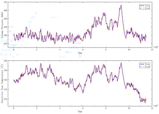
Figure 6.
Comparison of predicted and true values on the test set.
3.3. Gaussian Noise Data Test
In order to evaluate the performance of the model under suboptimal dataset conditions, normally distributed noise was incorporated into the dataset, with the process noise adhering to distribution υ~N (0,σ2). Noise with σ = 0.002 and σ = 0.005 was respectively applied to the dataset after normalization, followed by retraining and testing. The results of the training are presented in the Table 3, and Figure 7 illustrates the impact of noise on the prediction accuracy.
Table 3.
The RMSE and R2 under various noise conditions.
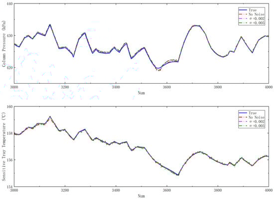
Figure 7.
Comparison of test results under noise data on the test set.
3.4. Model Predictive Control Using Predictive Model
Once a neural network model with adequate accuracy is obtained, it is integrated into the LMPC framework for the predictive control. The controller performance is evaluated through closed-loop disturbance tests and setpoint tracking tests, respectively, on both MPC and PID control systems. These two tests are capable of characterizing the control system’s ability to quickly stabilize against external disturbances in the closed-loop circuit, as well as its capability to respond rapidly to setpoint changes due to real-time optimization and production scheduling. The Integral Square Error (ISE) is employed to reflect the efficacy of the MPC, where the ISE is calculated by integrating the squared error over time for a single controlled variable. The calculation method for the ISE is as follows:
The closed-loop disturbance test involves introducing a perturbation of a 5 °C decrease in feed temperature. The closed-loop response curves are depicted in Figure 8. The ISE is calculated for the two controlled variables under the use of MPC and PID controllers, respectively, and the values are presented in Table 4.
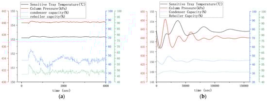
Figure 8.
Dynamic response curves of disturbance testing of distillation process: (a) MPC response curve; (b) PID response curve.
Table 4.
Disturbance test ISE of distillation process.
The PID control scheme, configured as column top pressure–column top cooling capacity and sensitive tray temperature–column bottom heating capacity, inherently causes significant lag and fails to stabilize rapidly. Modifying the control scheme to column top pressure–reflux flow rate may yield improvement. Due to the extended stabilization time, the calculation of the ISE for the PID controller is limited to the first 4000 s. Upon examining the response curves of the MPC controller, the disturbance in feed temperature has negligible impact on the column pressure and temperature, indicating a robust resistance to disturbances. Under the combined regulation of cooling and heating capacities, the heat is prematurely conducted into the column through the gas–liquid mass transfer process within the column, counteracting the effect of the temperature decrease.
In the setpoint tracking performance test, the setpoint of the column top pressure was increased by 5 kPa. The closed-loop response curves are depicted in Figure 9. The ISE was calculated for the two controlled variables under the use of MPC and PID controllers, respectively, and the values are presented in Table 5.
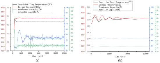
Figure 9.
Dynamic response curves of control point tracking testing of distillation process: (a) MPC response curve; (b) PID response curve.
Table 5.
Control point tracking test ISE of distillation process.
By analyzing the behavior of the MPC, it can be observed that upon a setpoint change, the cooling capacity at the column top rapidly decreases and the heating capacity swiftly increases to achieve a rapid rise in the overall column pressure, followed by a gradual adjustment of the cooling and heating capacities to a new steady state. In the setpoint tracking test, the PID controller takes nearly 100 times as long as the MPC controller to reach stability (correspondingly, the ISE integration time takes up to 10,000 s for this case), whereas the MPC controller achieves stability rapidly. The mass and heat transfer within the distillation column necessitate time, and the effect becomes more significant as the number of tray stages increases, leading to a significant time lag. Additionally, the presence of volume in the column bottom and reflux drum introduces the volume lag. For processes with such a substantial lag, the PID controller is unable to quickly stabilize the distillation column, whereas the MPC, by invoking the predictive model and utilizing multiple variables measured by a distributed control system, is capable of predicting the overall column conditions and responding swiftly and accurately to external changes.
By examining the log records generated during the control process, the prediction errors of the prediction model within the control process were compiled. Upon comparison, it was found that the prediction errors, as measured by the MAE (Mean Absolute Error), were all below 0.001. Due to the dynamic variation patterns of input variables during the prediction process being smoother than those in the test set, there were no instances of abrupt changes in other system parameters caused by sudden mutations in operational parameters. Consequently, the performance during the prediction process was superior to that of the test set.
In the MPC testing, it was observed that under the condition of utilizing a sufficiently accurate model, the MPC controller demonstrated robust performance against disturbances, as well as the capability to respond rapidly to commands from the scheduling layer. On one hand, this verifies the high precision and strong generalization ability of our process-mechanism-based deep neural network model. On the other hand, it also confirms that this model is fully applicable for tasks involving model predictive control.
The results of the testing were compared with similar studies, selecting the Simultaneous Multistep Transformer Architecture proposed by Park et al. [26], the physics-informed hybrid neural network model based on the Long Short-Term Memory (LSTM) neural network proposed by Zarzycki et al. [27], and the Neural Ordinary Differential Equation proposed by Luo et al. [28].
The Simultaneous Multistep Transformer Architecture proposed by Park et al. [26]. serves as a multistep prediction model. In their study, the transformer-based model was used for comparison with an LSTM-based model. Since the RMSE for each case was not listed in their study, we selected Case III: Temperature Control Lab Device for comparison, which involves a multivariate prediction task similar in form and difficulty to our established scenario. Firstly, in terms of accuracy, both the LSTM and transformer models in Park et al.’s study had MAEs above 1; in our study, the errors calculated during the control process were used to characterize the model’s multistep prediction performance, and the relative errors were converted to obtain the MAE, with all MAEs not exceeding 0.05. In terms of computational efficiency, although our proposed model is also based on RNN, it benefits from a neural network framework constructed on automatic differentiation and gradient backpropagation, which forms the MPC architecture. The solution speed for each MPC problem is within 2 s, which is significantly faster than the LSTM-based model used for comparison by Park et al., and comparable to the transformer model used for multistep prediction.
The physics-informed hybrid neural network model based on the Long Short-Term Memory (LSTM) neural network proposed by Zarzycki et al. [27]. is a data-driven modeling approach that incorporates process physical information, which shares some similarities with our approach. In the study by Zarzycki et al., a model was developed for a polymerization reactor to predict the Number-Average Molecular Weight (NAMW). As the model’s performance on the test set was not directly provided, and only the control process error was given without units, a direct comparison with our model is infeasible. In terms of computational speed, the model proposed by Zarzycki et al. exhibits rapid computation, completing a single iteration within approximately 140 milliseconds. This may be attributed to the fact that their study employed single-variable prediction, whereas our research involved multi-variable prediction, indicating a difference in model scale, as well as the efficiency of the employed MPC algorithms. Regarding the interpretability and extrapolation capabilities of the model, the Physics-Informed Neural Network (PINN) elegantly addresses this issue. In contrast to our study, which focuses on guiding the construction of data-driven models with process knowledge, the research by Zarzycki et al. presents a true hybrid model.
The Neural Ordinary Differential Equation proposed by Luo et al. [28]. is a novel deep neural network that integrates ordinary differential equations. In terms of model accuracy, the study by Luo et al. reported a Mean Squared Error (MSE) of 3.1 × 10⁻⁴ for datasets without noise. Since our research utilized Root Mean Squared Error (RMSE) for measurement, the converted MSE is 2.24 × 10⁻⁶, indicating significantly higher precision. For datasets with noise, due to the inability to quantify the relative scale of noise for comparison, the following are provided for reference only. The model proposed by Luo et al. yielded an MSE of 0.0068 at a 2% noise level and an MSE of 0.03 at a 6% noise level. In contrast, our model achieved an MSE of 1.15 × 10⁻⁵ at a 0.2% noise level and an MSE of 4.16 × 10⁻⁵ at a 0.5% noise level.
Relative to the model proposed by Luo et al. [28], our model exhibits slight deficiencies in computational speed and resistance to noise, which identifies areas for potential improvement in our research.
4. Conclusions
This study proposes a deep neural network model based on a process mechanism and applies it to the predictive control of distillation processes. Initially, a neural network sub-model based on the GRU + attention mechanism is constructed, with the input–output relationship for machine learning determined according to the mechanism equations of chemical unit operation models. Furthermore, based on the principles of solving ordinary differential equations (ODEs) in mechanism models, improvement strategies such as a Distribution net and Residual connections are proposed. Comparative experiments are designed with four neural network architectures, and the results indicate that the model’s accuracy is significantly enhanced after employing the aforementioned improvement strategies. Compared to the RNN-only model, the mean squared error is reduced by 77.2%.
The well-trained model is applied to the predictive control of distillation columns. When compared to the PID control, the integral squared error (ISE) for key variables is significantly decreased in both closed-loop disturbance tests and setpoint tracking tests. For instance, the ISE of our model is reduced by 98.8% compared to the PID control in sensitive tray temperature control, and by 90.3% in the column pressure control. This fully demonstrates the high efficiency and practicality of the model in the control of distillation processes.
In summary, the model proposed in this study is capable of fitting the complex nonlinear behavior of chemical systems with high precision and exhibits strong generalization capabilities. It can serve as a general framework for predictive applications in various unit operations and plant systems. Future research will focus on the optimization of the model structure, expanding its application in more complex industrial processes, and exploring its potential in real-time optimization and fault diagnosis to enhance the overall benefits and safety of industrial production.
Author Contributions
Conceptualization, Z.W.; Methodology, Z.W.; Software, Z.W.; Validation, Z.W. and H.W.; Formal analysis, Z.W.; Resources, Z.W. and H.W.; Data curation, Z.W. and H.W.; Writing—original draft preparation, Z.W.; Writing—review and editing, Z.W., H.W., and Z.D.; Visualization, Z.W. and H.W.; Project administration, Z.W. and Z.D.; Funding acquisition, Z.D. All authors have read and agreed to the published version of the manuscript.
Funding
This research received no external funding.
Data Availability Statement
Data are contained within the article.
Acknowledgments
The authors thank the editors and reviewers for their helpful comments regarding the manuscript and other individuals who contributed but are not listed as authors of this study.
Conflicts of Interest
The authors declare no conflicts of interest.
Abbreviations
The following abbreviations are used in this manuscript:
| PID | Proportional-Integral-Derivative Control |
| MPC | Model Predictive Control |
| NMPC | Nonlinear Model Predictive Control |
| CSTR | Continuous Stirred Tank Reactor |
| RNN | Recurrent Neural Network |
| GRU | Gated Recurrent Unit |
| FNN | Feedforward Neural Network |
| MLP | Multilayer Perception |
| ELU | Exponential Linear Unit |
| RELU | Rectified Linear Unit |
| NLP | Natural Language Processing |
| ODE | Ordinary Differential Equation |
| PDE | Partial Differential Equation |
| LMPC | Lyapunov-based Model Predictive Control |
| ISE | Integral Square Error |
References
- Pallavicini, J.; Fedeli, M.; Scolieri, G.D.; Tagliaferri, F.; Parolin, J.; Sironi, S.; Manenti, F. Digital Twin-Based Optimization and Demo-Scale Validation of Absorption Columns Using Sodium Hydroxide/Water Mixtures for the Purification of Biogas Streams Subject to Impurity Fluctuations. Renew. Energy 2023, 219, 119466. [Google Scholar] [CrossRef]
- Min, Q.; Lu, Y.; Liu, Z.; Su, C.; Wang, B. Machine Learning Based Digital Twin Framework for Production Optimization in Petrochemical Industry. Int. J. Inf. Manag. 2019, 49, 502–519. [Google Scholar] [CrossRef]
- Tanaka, M.; Koyama, K.; Shibata, J. Steady-State Local Linearization of the Countercurrent Multistage Extraction Process for Metal Ions. Ind. Eng. Chem. Res. 1997, 36, 4353–4357. [Google Scholar] [CrossRef]
- Zhang, C.; Vasudevan, S.; Rangaiah, G.P. Plantwide Control System Design and Performance Evaluation for Ammonia Synthesis Process. Ind. Eng. Chem. Res. 2010, 49, 12538–12547. [Google Scholar] [CrossRef]
- Gao, S.; Bo, C.; Jiang, C.; Zhang, Q.; Yang, G.; Chu, J. Hybrid Modeling for Carbon Monoxide Gas-Phase Catalytic Coupling to Synthesize Dimethyl Oxalate Process. Chin. J. Chem. Eng. 2024, 70, 234–250. [Google Scholar] [CrossRef]
- Savage, T.; Almeida-Trasvina, H.F.; del Río-Chanona, E.A.; Smith, R.; Zhang, D. An Adaptive Data-Driven Modelling and Optimization Framework for Complex Chemical Process Design. In Computer Aided Chemical Engineering; Pierucci, S., Manenti, F., Bozzano, G.L., Manca, D., Eds.; 30 European Symposium on Computer Aided Process Engineering; Elsevier: Amsterdam, The Netherlands, 2020; Volume 48, pp. 73–78. [Google Scholar] [CrossRef]
- Chen, Y.; Yu, H.; Liu, C.; Xie, J.; Han, J.; Dai, H. Synergistic Fusion of Physical Modeling and Data-Driven Approaches for Parameter Inference to Enzymatic Biodiesel Production System. Appl. Energy 2024, 373, 123874. [Google Scholar] [CrossRef]
- Alauddin, M.; Khan, F.; Imtiaz, S.; Ahmed, S.; Amyotte, P. Integrating process dynamics in data-driven models of chemical processing systems. Process Saf. Environ. Prot. 2023, 174, 158–168. [Google Scholar] [CrossRef]
- Sharma, N.; Singh, K. Model Predictive Control and Neural Network Predictive Control of TAME Reactive Distillation Column. Chem. Eng. Process. Process Intensif. 2012, 59, 9–21. [Google Scholar] [CrossRef]
- Li, S.; Li, Y.-Y. Neural Network Based Nonlinear Model Predictive Control for an Intensified Continuous Reactor. Chem. Eng. Process. Process Intensif. 2015, 96, 14–27. [Google Scholar] [CrossRef]
- Jian, N.L.; Zabiri, H.; Ramasamy, M. Data-Based Modeling of a Nonexplicit Two-Time Scale Process via Multiple Time-Scale Recurrent Neural Networks. Ind. Eng. Chem. Res. 2022, 61, 9356–9365. [Google Scholar] [CrossRef]
- Rebello, C.M.; Marrocos, P.H.; Costa, E.A.; Santana, V.V.; Rodrigues, A.E.; Ribeiro, A.M.; Nogueira, I.B.R. Machine Learning-Based Dynamic Modeling for Process Engineering Applications: A Guideline for Simulation and Prediction from Perceptron to Deep Learning. Processes 2022, 10, 250. [Google Scholar] [CrossRef]
- Xu, B.; Wang, Y.; Meng, Z.; Chen, Y.; Yin, S. An Intelligent Identification Method Based on Self-Adaptive Mechanism Regulated Neural Network for Chemical Process. J. Taiwan Inst. Chem. Eng. 2024, 155, 105318. [Google Scholar] [CrossRef]
- Bikmukhametov, T.; Jäschke, J. Combining Machine Learning and Process Engineering Physics towards Enhanced Accuracy and Explainability of Data-Driven Models. Comput. Chem. Eng. 2020, 138, 106834. [Google Scholar] [CrossRef]
- Sun, B.; Yang, C.; Wang, Y.; Gui, W.; Craig, I.; Olivier, L. A Comprehensive Hybrid First Principles/Machine Learning Modeling Framework for Complex Industrial Processes. J. Process Control 2020, 86, 30–43. [Google Scholar] [CrossRef]
- Li, Y.; Li, N.; Ren, J.; Shen, W. An Interpretable Light Attention–Convolution–Gate Recurrent Unit Architecture for the Highly Accurate Modeling of Actual Chemical Dynamic Processes. Engineering 2024, 39, 104–116. [Google Scholar] [CrossRef]
- Bradley, W.; Kim, J.; Kilwein, Z.; Blakely, L.; Eydenberg, M.; Jalvin, J.; Laird, C.; Boukouvala, F. Perspectives on the Integration between First-Principles and Data-Driven Modeling. Comput. Chem. Eng. 2022, 166, 107898. [Google Scholar] [CrossRef]
- Vaswani, A.; Shazeer, N.; Parmar, N.; Uszkoreit, J.; Jones, L.; Gomez, A.N.; Kaiser, L.; Polosukhin, I. Attention Is All You Need. arXiv 2023, arXiv:1706.03762. [Google Scholar] [CrossRef]
- He, K.; Zhang, X.; Ren, S.; Sun, J. Deep Residual Learning for Image Recognition. In Proceedings of the 2016 IEEE Conference on Computer Vision and Pattern Recognition (CVPR), Las Vegas, NV, USA, 27–30 June 2016; pp. 770–778. [Google Scholar] [CrossRef]
- E, W. A Proposal on Machine Learning via Dynamical Systems. Commun. Math. Stat. 2017, 5, 1–11. [Google Scholar] [CrossRef]
- Ruthotto, L.; Haber, E. Deep Neural Networks Motivated by Partial Differential Equations. arXiv 2018, arXiv:1804.04272. [Google Scholar] [CrossRef]
- Wu, Z.; Tran, A.; Rincon, D.; Christofides, P.D. Machine Learning-based Predictive Control of Nonlinear Processes. Part I: Theory. AIChE J. 2019, 65, e16729. [Google Scholar] [CrossRef]
- Wu, Z.; Rincon, D.; Christofides, P.D. Process Structure-Based Recurrent Neural Network Modeling for Model Predictive Control of Nonlinear Processes. J. Process Control 2020, 89, 74–84. [Google Scholar] [CrossRef]
- Kingma, D.P.; Ba, J. Adam: A Method for Stochastic Optimization. arXiv 2014, arXiv:1412.6980. [Google Scholar]
- Murthy Konda, N.V.S.N.; Rangaiah, G.P.; Krishnaswamy, P.R. A Simple and Effective Procedure for Control Degrees of Freedom. Chem. Eng. Sci. 2006, 61, 1184–1194. [Google Scholar] [CrossRef]
- Park, J.; Babaei, M.R.; Munoz, S.A.; Venkat, A.N.; Hedengren, J.D. Simultaneous multistep transformer architecture for model predictive control. Comput. Chem. Eng. 2023, 178, 108396. [Google Scholar] [CrossRef]
- Zarzycki, K.; Ławryńczuk, M. Long short-term memory neural networks for modeling dynamical processes and predictive control: A hybrid physics-informed approach. Sensors 2023, 23, 8898. [Google Scholar] [CrossRef]
- Luo, J.; Abdullah, F.; Christofides, P.D. Model predictive control of nonlinear processes using neural ordinary differential equation models. Comput. Chem. Eng. 2023, 178, 108367. [Google Scholar] [CrossRef]
Disclaimer/Publisher’s Note: The statements, opinions and data contained in all publications are solely those of the individual author(s) and contributor(s) and not of MDPI and/or the editor(s). MDPI and/or the editor(s) disclaim responsibility for any injury to people or property resulting from any ideas, methods, instructions or products referred to in the content. |
© 2025 by the authors. Licensee MDPI, Basel, Switzerland. This article is an open access article distributed under the terms and conditions of the Creative Commons Attribution (CC BY) license (https://creativecommons.org/licenses/by/4.0/).