The Dynamic Mechanical Response of Anchored Fissured Rock Masses at Different Fissure Angles: A Coupled Finite Difference–Discrete Element Method

Abstract

Anchored surrounding rock is prone to large nonlinear deformation and instability failure under dynamic disturbances. The fissures and defects within the surrounding rock make the rock mass’s bearing characteristics and deformation instability behavior increasingly complex. To investigate the effect of the fissure angle on the dynamic mechanical response of the anchored body, a dynamic loading model of the anchored, fissured surrounding rock unit body was established based on the finite difference–discrete element coupling method. The main conclusions are as follows: Compared to the indoor test results, this numerical model can accurately simulate the dynamic response characteristics of the unit body. As the fissure angle increased, the dynamic strength, failure strain, and dynamic elastic modulus of the specimen generally decreased and then increased, with a critical angle at approximately 45°. Compared to 0°, when the fissure angle was 45°, the dynamic strength, failure strain, and dynamic elastic modulus decreased by 17.08%, 15.48%, and 9.11%, respectively. Additionally, the evolution process of cracks and fragments shows that the larger the fissure angle, the more likely cracks are to develop along the initial fissure direction, which then triggers the formation of tensile cracks in other regions. Increasing the fissure angle causes the specimen to rupture earlier, making the main rupture plane more directional.

1. Introduction

Ensuring the safety and stability of fissured surrounding rock is crucial during the construction and operation of underground engineering projects [1,2]. As one commonly used method for controlling the stability of the surrounding rock, bolt support has evolved into various techniques centered around anchor bolts over the years. Anchorage technology forms an effective system between the rock mass and the anchor cables, fully utilizing the bearing characteristics of the anchor bolts and rock mass while minimizing the disturbance to the rock mass and avoiding significant secondary damage [3,4]. However, the surrounding rock is often not intact due to excavation unloading and construction disturbance, but instead consists of a fissured rock mass. The load experienced by fissured, anchored rock masses is not limited to static loads, and impact loads should not be overlooked [5]. In addition, the nonlinear and anisotropic characteristics [6,7] of fissured rock masses make their bearing properties and deformation instability behaviors more complex, and the fissure structure itself should also be considered. Especially under the disturbance caused by impact loading, ensuring the safety and stability of the fissured, anchored surrounding rock is crucial (Figure 1). Understanding the mechanical behavior, fracture evolution, and anchor bolt deformation mechanisms of the anchored, fissured surrounding rock under dynamic loading is fundamental to ensuring the safe and efficient operation of underground engineering.

The structural characteristics of fissures directly influence the bearing and deformation properties of rocks, such as the fissure length [8,9], roughness [10,11], density [12,13], and angle, among others [14]. Xia et al. [15] reported the effect of the fissure angle on the compressive strength of sandstone. As the fissure angle increased, the compressive strength and elastic modulus showed an asymmetric U-shaped trend, with the failure mode being a mixed tensile–shear failure. Kang et al. [16] conducted cyclic loading and unloading tests on sandstone specimens with fissures under complex stress paths at different angles. From an energy perspective, they found that as the fissure angle increases, the rock’s energy storage coefficient increases while the energy dissipation coefficient decreases, indicating a higher bearing capacity of the rock. The influence of the fissure angle is not only observed in a static state but also affects the dynamic mechanical response. Liu et al. [17] reported the dynamic failure process of single-fissure rocks with different fissure angles under dynamic loading. They found that a greater inclination angle leads to more cracks during failure. Yan et al. [18] conducted static–dynamic coupled loading on rocks with multiple defects and found that as the fissure angle increased from 15° to 60°, the failure mode transitioned from mixed tensile–shear cracking to mixed compressive–shear cracking.

The influence of the inclination angle of defects (such as fissures, bedding planes, and notches) is also reflected in the anchored rock mass. Yang et al. [7] studied the strength and deformation behavior of anchored joint samples and found that for joint samples with crack inclination angles ranging from 0° to 90°, the peak strength and elastic modulus decrease and then increase. Sun et al. [19] investigated the anchoring performance of conventional bolts and constant-resistance large-deformation bolts in rock masses, revealing that variations in the inclination angle can influence the failure mode of the anchored rock mass. Wen et al. [20] performed uniaxial compression tests on double-fissure anchored granite and determined that the fissure inclination angle affects the influence of anchor bolts on rock deformation control and strength enhancement. Similarly, the dynamic response behavior of anchored fissure units with varying inclination angles has attracted significant attention. For example, using numerical simulation, Chen et al. [21] discussed the reinforcement and crack arrest mechanisms of anchored, fissured granite at different angles. Fan et al. [22] determined the optimal anchoring angle for anchored units by analyzing the dynamic mechanical properties, strain rate evolution, and energy dissipation of anchor–fissure units.

However, the above studies mainly focused on the overall bearing capacity of the unit, with limited research on the mechanisms of fissure evolution, the anchor force, and deformation characteristics. In addition, traditional single-simulation methods struggle to simultaneously model both the specimen’s fragmentation and discrete failure and the rod elements’ elastic deformation. The coupling simulation method based on PFC and FLAC software is becoming an important tool for addressing such issues [23,24]. Therefore, this work focuses on the anchored, fissured surrounding rock unit as the research object, using rock-like anchoring units as prototypes. Based on a finite difference–discrete element coupled numerical method, a dynamic loading numerical model for anchored fissure units was constructed, and the influence of the fissure angle on the dynamic mechanical properties, fissure evolution, and anchor force–deformation behavior of the anchored fissure units is discussed.

2. Methodology

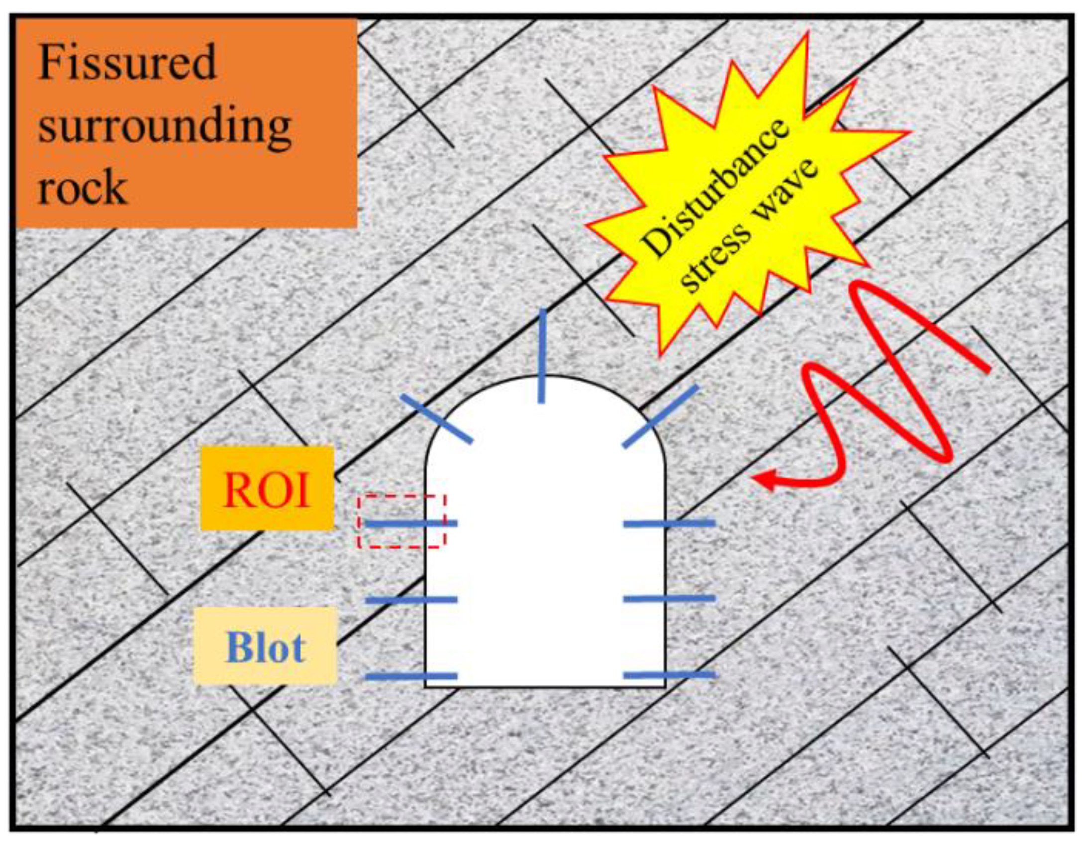
2.1. Experimental Design of Numerical Simulation for Simplified Element

To investigate the effect of the fissure distribution angle on the dynamic bearing characteristics of the anchored, fissured rock mass, a rock-like anchored, fissured specimen was used as the prototype. Based on the unit body of the anchored, fissured surrounding rock mass (as shown in the ROI in Figure 1), a rectangular prism containing a single fissure (dimensions: length of 80 mm, width of 40 mm, height of 80 mm; shown in Figure 2) was selected as the research object. The morphology of the fissure rupture surface was modeled after the actual rupture surface from a sandstone true triaxial unloading test (with the main rupture surface forming a 20° angle with the horizontal plane). The fissure distribution angle in the rock mass was adjusted by rotating the rupture surface. The anchor bolt had a diameter of 5 mm, a length of 100 mm, and an initial anchoring preload of 2.5 kN. Seven different operating conditions were set, with fissure angles of 0°, 15°, 30°, 45°, 60°, 75°, and 80°. At a fissure angle of 90°, the fissure coincides with the anchor bolt, rendering the anchoring effect ineffective. Therefore, the last group of conditions was assigned an angle of 85°.

The prototype of the indoor similitude sample for the anchored, fissured rock body was sandstone taken from a tunnel in the Shoushan No. 1 Mine in Henan Province, China. It was cast using cement (P.O 42.5), silica fume, quartz sand, and water (the final mix ratio of 1: 0.01: 0.8: 0.45 was determined through an orthogonal ratio experiment by comparing key mechanical and deformation parameters). After curing, pre-drilling was conducted using a drilling machine. Anchoring was then performed using trays (side length of 20 mm, thickness of 1.5 mm), opening gaskets (side length of 20 mm, thickness of 1.0 mm), and threaded rods (diameter of 5 mm, length of 160 mm). Grouting reinforcement was performed using cement mortar with a water-to-cement ratio of 0.45, with a pre-tension force of 2.5 kN applied using a torque wrench. The anchor rod was made of M5 low-carbon steel, with a measured yield load of 6775.98 N (strain: 1.65%) and a peak load of 7111.23 N (strain: 9.05%).

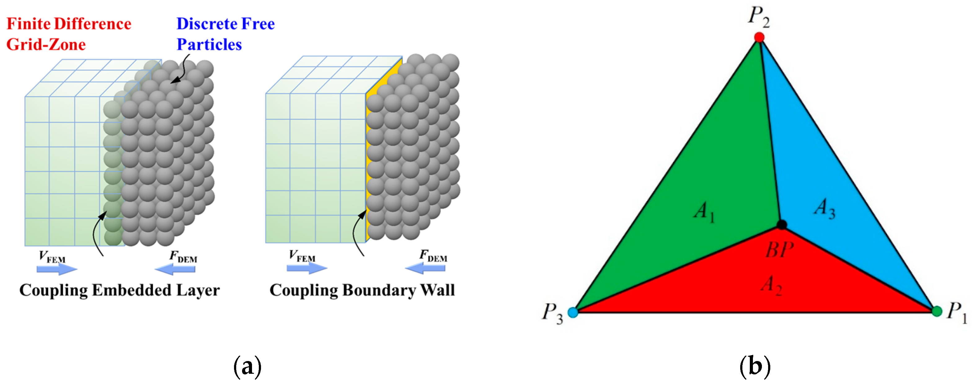
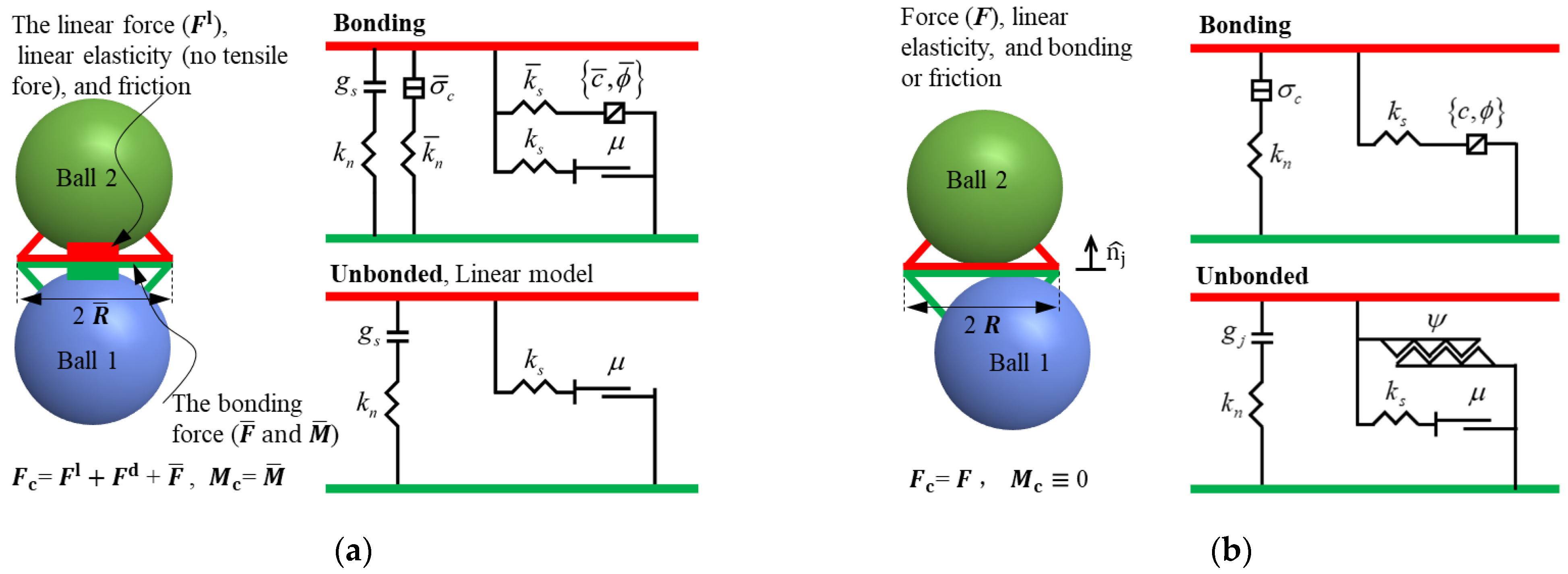
2.2. Finite Difference–Discrete Element Coupling Methods: Basic Principles

In numerical analysis, the Finite Difference Method (FDM) [25] is a grid-based numerical calculation method that solves continuum mechanics equations using the explicit Lagrangian algorithm through time-stepping, simulating continuous media’s deformation, stress distribution, and failure behavior. However, due to the constraints of adjacent elements, the deformation of elements in a local region cannot be too large; otherwise, the model may fail to converge, leading to the termination of the solution process. The Discrete Element Method (DEM) [26] discretizes the specimen into individual particle units, describing the overall behavior through inter-particle contact forces and displacements. It has distinct advantages in simulating engineering cases with large deformations. However, due to computational performance limitations, the model’s excessive number of blocks or particles significantly reduces the solving efficiency. Therefore, this work combined continuous and discrete analysis methods. The Discrete Element Method was used for detailed simulation in regions with large deformations that needed focused study, while the continuous analysis method was employed in non-critical regions with small deformations. This approach prevented solution failure caused by large deformations while significantly enhancing the computational efficiency [27].

In PFC software (PFC3D 6.00.30, Itasca Consulting Group, Minneapolis, MN, United States, 2021), coupled analysis using FLAC mainly involves two methods (Figure 3a): Wall–Zone coupling and Ball–Zone coupling [28,29]. The former is generally used for analyzing engineering cases with small deformations, while the latter is commonly used for analyzing problems with large deformations, such as earthquakes [27]. To ensure the smooth implementation of coupled analysis, the particles in PFC and the continuous region in FLAC must transfer forces and displacements through a wall composed of multiple triangular faces. When a ball particle contacts a triangular face at point B, assume that BP is the closest point on the face to B, and the vectors from this point to the three vertices of the triangular face are denoted as (i = 1, 2, 3), as shown in Figure 3b. If the force and moment at the contact point B are denoted as $\overrightarrow{F}$ and ${\overrightarrow{M}}_{\mathrm{b}}$, respectively, the total moment on the triangular face can be expressed as follows [30]:

$$\overrightarrow{M}={\overrightarrow{M}}_{\mathrm{b}}+(B-BP)\times \overrightarrow{F}$$

(1)

The equivalent force on the coupled triangular face can also be expressed as [30]

$${\displaystyle {\sum }_1^3{\overrightarrow{F}}_i}=\overrightarrow{F}$$

(2)

$${\displaystyle {\sum }_1^3{\overrightarrow{L}}_i\times {\overrightarrow{F}}_i}=\overrightarrow{M}$$

(3)

In the local coordinate system defined by the triangular face, where the x-axis and y-axis correspond to the normal and tangential vectors of the entire wall, respectively, the following relationship is established [30]:

$${{\displaystyle \sum \overrightarrow{F}}}_{i,x}={\overrightarrow{F}}_x$$

(4)

$${{\displaystyle \sum \overrightarrow{F}}}_{i,y}={\overrightarrow{F}}_y$$

(5)

$${\displaystyle \sum {\overrightarrow{F}}_{i,z}}={\overrightarrow{F}}_z=0$$

(6)

$${\displaystyle \sum \left({\overrightarrow{L}}_{i,y}\times {\overrightarrow{F}}_{i,z}-{\overrightarrow{L}}_{i,z}\times {\overrightarrow{F}}_{i,y}\right)}={\overrightarrow{M}}_x$$

(7)

$${\displaystyle \sum \left({\overrightarrow{L}}_{i,z}\times {\overrightarrow{F}}_{i,x}-{\overrightarrow{L}}_{i,x}\times {\overrightarrow{F}}_{i,z}\right)}={\overrightarrow{M}}_y$$

(8)

$${\displaystyle \sum \left({\overrightarrow{L}}_{i,x}\times {\overrightarrow{F}}_{i,y}-{\overrightarrow{L}}_{i,y}\times {\overrightarrow{F}}_{i,x}\right)}={\overrightarrow{M}}_z$$

(9)

Since the number of unknowns in Equation (9) exceeds the number of equations, a unique solution cannot be obtained directly. Therefore, an additional constraint equation must be introduced. Since the sum of the dot products of the vertex vectors in the z-direction of the local coordinate system is zero, the additional constraint equation is derived as [30]

$${\displaystyle \sum \left({\overrightarrow{L}}_{i,z}\times {\overrightarrow{F}}_{i,z}\right)=0}$$

(10)

2.3. Model Construction and Selection of Basic Parameters

The dynamic loading numerical model of the anchored, fissured rock mass is illustrated in Figure 4. The rock-like matrix was simulated using spherical particles with a particular bond strength, while the loading rods and anchor rods were modeled using zone elements in FLAC. The scanned, actual fracture surfaces were imported into PFC in geometry form and set as fractures for simulating fissures. The contact model between the rock-like matrix particles was chosen to be the parallel bond model (PBM) [31], while the contact model at the fractures was chosen to be the smooth joint model (SJM) [32], as shown in Figure 5. The diameter of the anchor rod and the dimensions of the tray in the anchored sample matched those in the laboratory specimen (anchor rod diameter of 5 mm, tray dimensions of 20 mm × 20 mm × 2.5 mm). A 6 mm hole was drilled in the specimen, and small-diameter spherical particles were used to fill the gap between the anchor rod and the sample (simulating grouting). The bond model between the particles was also the PBM (in Figure 5a). The basic properties of the particles are listed in

Table 1. Basic properties of particles in rock matrix and grouting area.

Basic Properties of Rock-Like Matrix Particles	Value	Basic Properties of Particles in the Grouting Zone	Value
Radius range/mm	1.00~1.66	Radius range/mm	0.10~0.25
Porosity	0.30	Porosity	0.30
Density/kg/m3	2110.00	Density/kg/m3	1800.00

. The particle radius range was selected based on the size relationship between the materials and relevant studies on particle size selection. Ultimately, the particle radius range was determined to be 1–1.66 mm, resulting in 14,587 particles in the generated model.

Based on the strain data of the anchor rod monitored during the indoor dynamic impact test, it was evident that the anchor rod did not reach yielding during the impact process. As a result, a linear constitutive model could be employed to simulate the force and deformation of the anchor rod before yielding. The “trial-and-error method” [33] was applied to iteratively adjust the relevant parameters in the linear constitutive model to align with the linear elastic phase from the indoor tensile test of the anchor rod. The results, obtained by selecting a density of 7800 kg/m³, an elastic modulus of 31.9 GPa, and a Poisson’s ratio of 0.3, are presented in Figure 6. These results closely match the linear elastic phase from the indoor test, indicating that the calibrated parameters accurately represent the anchor rod’s force and deformation behavior.

The diameter of the bars in the SHPB system was 100 mm, with both the incident and transmission bars having lengths of 3000 mm. The constitutive models of these bars were chosen to be elastic models, with their material properties matching those of the indoor experiment: a density of 7800 kg/m³, elastic modulus of 210 GPa, and Poisson’s ratio of 0.29. Three monitoring points were set on the incident and transmission bars to track the propagation of the stress wave in the bars. Points #1 and #6, #2 and #5, and #3 and #4 were located 2000 mm, 1500 mm, and 1000 mm from the left and right sides of the specimen, respectively, as shown in Figure 4.

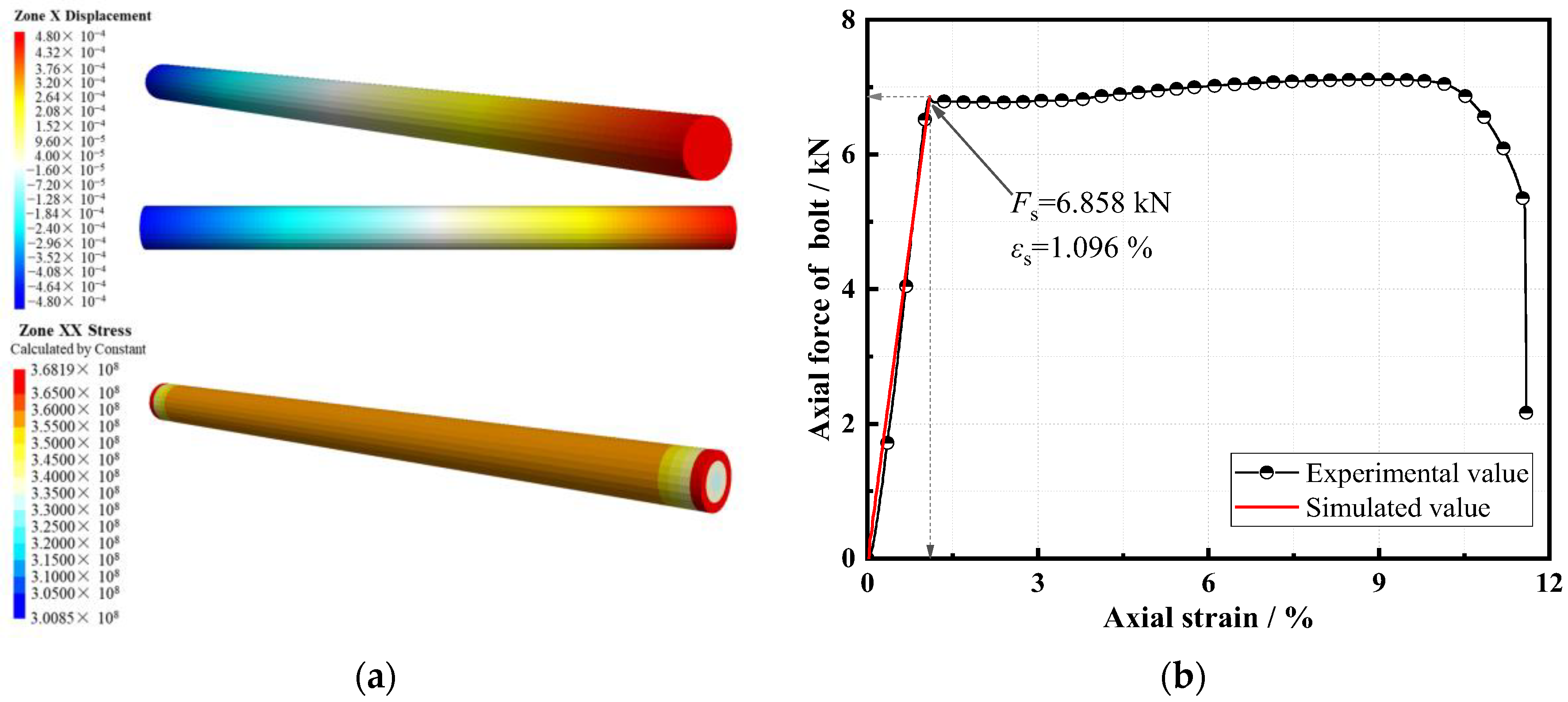
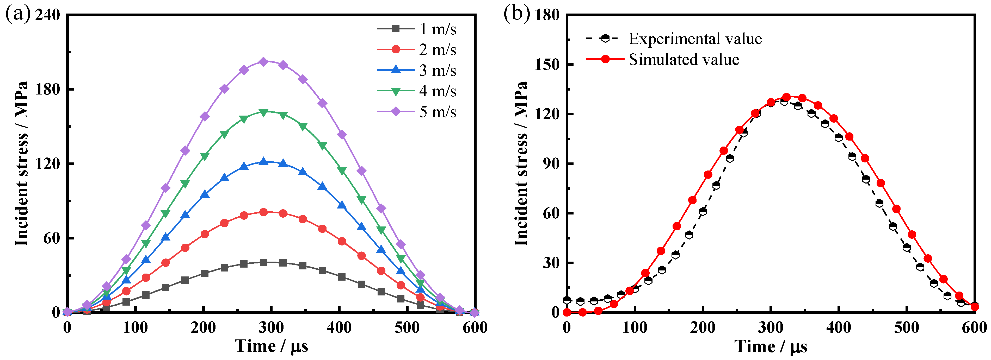
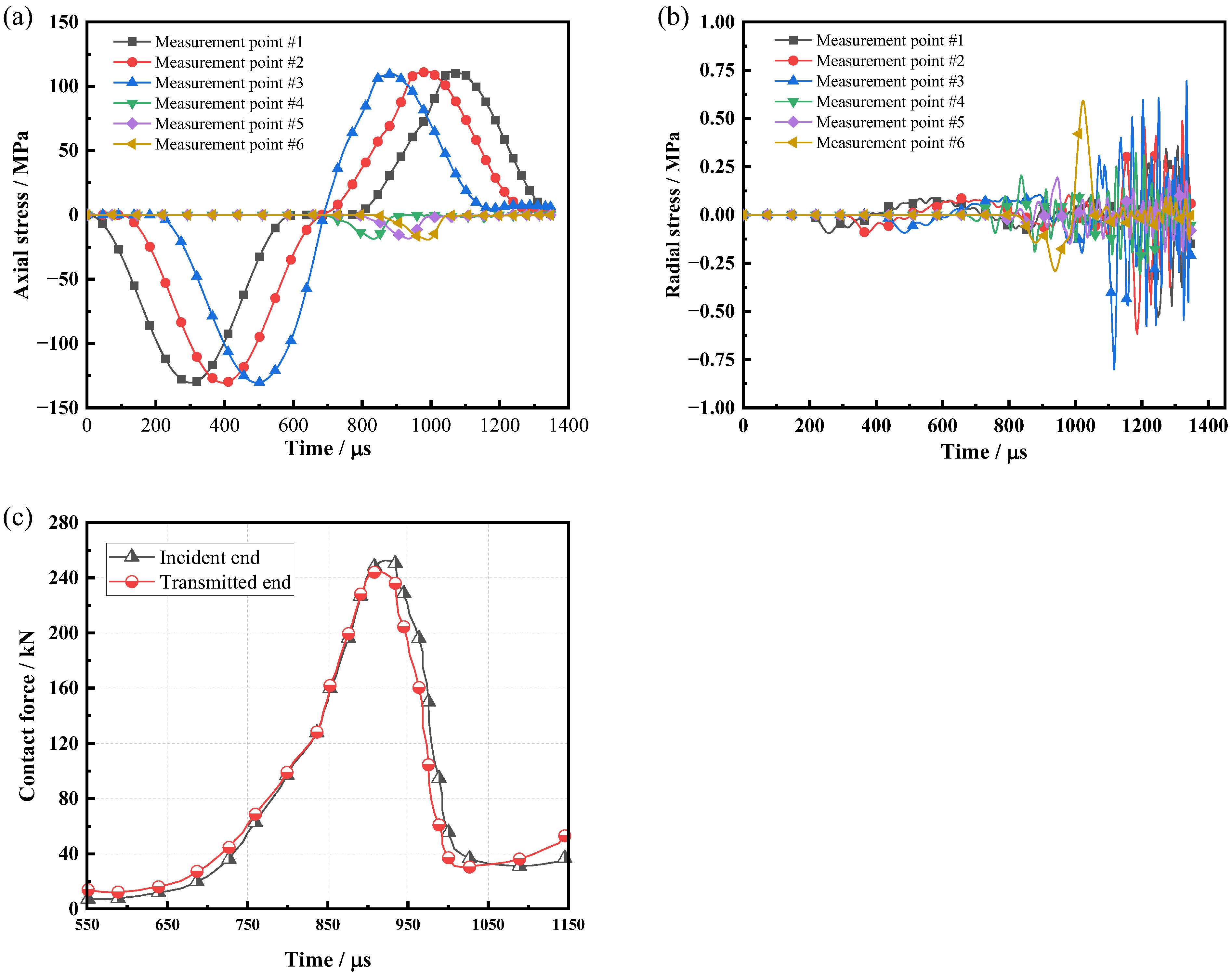
2.4. Loading Method and Model Validity Verification

To mitigate the dispersion effect during the stress wave propagation process, many researchers utilize PFC software to simulate the SHPB dynamic impact test, typically incorporating a waveform shaper or constructing a conical-shaped projectile between the bullet and the incident bar [34,35]. This approach can achieve the desired outcome by shaping the stress wave to resemble a sinusoidal form. However, in numerical simulations, the period of the stress wave generated after the impact is challenging to control, requiring adjustments to the bar length to match experimental waveforms. Since the loading bars were modeled via FLAC-PFC coupling, the dynamic load application method in FLAC was used to apply the stress wave.

In FLAC, dynamic loads can be applied at the model boundaries or nodes in various forms, such as the velocity, acceleration, and stress. To better replicate the laboratory test scenario, this study applied the impact disturbance load using the velocity on the incident bar side. The fundamental procedure was as follows: First, the bar boundary was set to static, and the dynamic module was activated. A half-cosine wave velocity was then applied on the incident bar side using a custom Fish function. After one stress wave period, the cosine wave at the incident end was removed, and the boundary was set to static. At this point, the stress wave was divided into transmitted and reflected waves at the specimen boundary, simulating the dynamic impact test.

Specifically, the dynamic load was applied to the incident section surface with the “Zone face apply velocity-x” command in FLAC, while the half-cosine stress wave was introduced through the Fish function. Varying incident stresses could be generated by adjusting the dynamic load velocities. By adjusting the dynamic load velocity, the results could be matched with those from the laboratory tests, establishing a relationship between the dynamic load velocity and strain rate. The formula for the half-cosine stress wave, implemented via the Fish function, is presented below:

$$\left\{\begin{array}{l}P=0 (t>T)\\ P={\displaystyle \frac{1}{2}}(1-\cos ({\displaystyle \frac{2\pi }{T}}t)) (t<T)\end{array}\right.$$

(11)

In the equation, T represents the duration of the applied half-cosine wave, i.e., the period. Based on the results of the laboratory tests, the duration of the incident wave was approximately 600 μs, so 600 μs was used as the duration of the half-cosine wave in the simulation. The time history curve of the incident stress wave after applying the velocity is shown in Figure 7a.

The peak of the incident rod stress wave was modified by altering the dynamic loading velocity. With an increase in the velocity, the incident stress progressively rose. At a velocity of 1 m/s, the peak stress of the incident wave was approximately 40 MPa; as the velocity reached 5 m/s, the peak stress rose to approximately 200 MPa. Based on the trend in the peak incident stress concerning the velocity, it was easy to match the dynamic loading velocity corresponding to different strain rates (impact gas pressure) that aligned with the peak incident stress in the laboratory tests. Figure 7b shows the numerical simulation of the incident stress wave for three specimens under a 0.4 MPa impact gas pressure, based on the peak incident stress. Under these conditions, the dynamic loading velocity in the numerical simulation was 3.29 m/s. It is evident that the aforementioned half-cosine stress wave application method accurately matched both the peak and shape of the incident stress wave and effectively reproduced its wavelength.

To validate the constructed loading model, it was essential to verify if the stress wave propagation met the following two conditions: the one-dimensional stress wave assumption and the homogeneity assumption. Figure 8 shows the axial and radial stress time histories at different measurement points during the loading process. As shown in Figure 8a, the axial stress waves at different measurement points had good consistency in both their waveform and amplitude, with the stress waveforms presenting a sinusoidal shape. The radial stress fluctuated over time without a discernible pattern (as shown in Figure 8b), with the maximum stress wave amplitude not exceeding 1 MPa, significantly smaller than the axial stress. This phenomenon indicates that the stress wave mainly propagated along the axial direction, with minimal attenuation and dispersion effects. Therefore, the assumption of one-dimensional stress wave propagation was valid. Furthermore, the contact between the specimen and the rod end was verified, and the stress on both sides was found to be in good agreement (as shown in Figure 8c), confirming the model’s dynamic force balance and validating the homogeneity assumption.

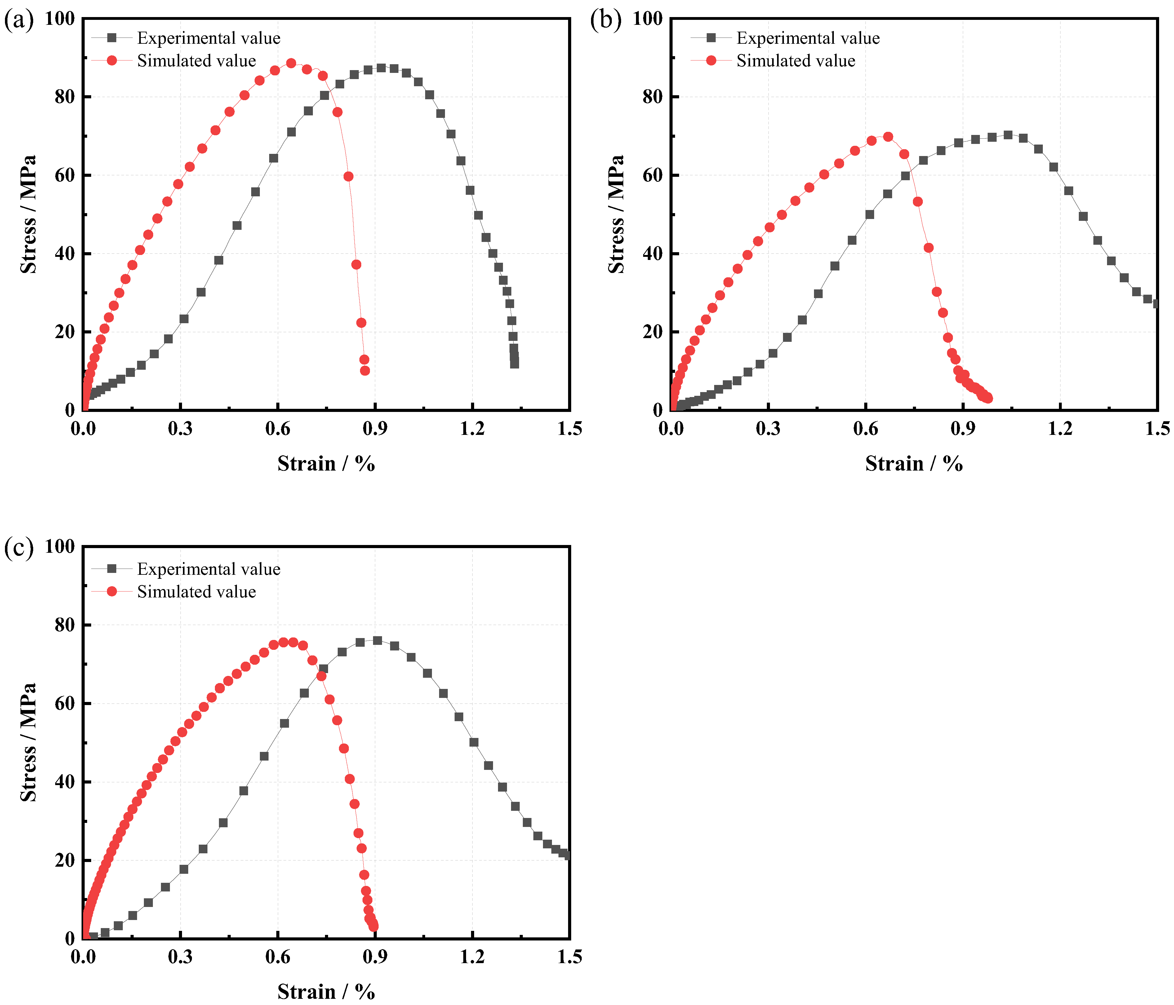
2.5. Particle Microscopic Parameter Calibration

Upon establishing the loading model, parameter calibration was performed on the intact, fissured, and anchored specimens to obtain the bond parameters between particles in the rock-like matrix, the bond parameters at the fracture sites, and the bond parameters in the grouting region. The specific steps were as follows: (I) We simulated the intact specimen under a 0.4 MPa gas pressure impact, where the bond parameters between particles in the rock-like matrix were determined through “the trial-and-error method”. (II) We simulated the fissured specimen under a 0.4 MPa gas pressure impact. The above-determined bond parameters were assigned to the particles in the rock-like matrix. The bond parameters at the fracture sites were then calibrated using the “the trial-and-error method”. (III) We performed a dynamic impact loading simulation of the anchored sample under the same 0.4 MPa gas pressure impact as in the laboratory test, assigning the above-determined parameters to the particles in the rock-like matrix and at the fracture sites and calibrating the bond parameters in the grouting region using the “trial and error method”.

Calibrating the bond parameters in PFC is a highly complex task, and “the trial-and-error method” is frequently employed for this purpose. To expedite the matching of the mesoscopic parameters, relevant calibration methods from previous studies were reviewed and modified before initiating the calibration process. During the calibration process, the bond parameters between the particles were initially set to high values. The mesoscopic elastic modulus was then adjusted continuously to match the elastic modulus obtained from the laboratory tests. Then, the normal-to-tangential-stiffness ratio was adjusted to correct Poisson’s ratio; the tensile strength and cohesion were changed in constant proportions to calibrate the peak stress. Finally, the friction coefficient was adjusted to simulate the post-peak characteristics of the curve.

Figure 9 illustrates the stress–strain curves of various specimens obtained from the simulation. The bond parameters between different types of medium particles after calibration are shown in

Table 2. Particle bonding parameters of various materials.

Microscopic Parameters	Rock-Like Matrix	Grouting Region	Fissure
Normal stifness (GPa/m)	—	—	1200
Tangential stiffness (GPa/m)	—	—	1200
Effective elastic modulus (GPa)	12.0	10.5	—
Ratio of normal to tangential stiffness	2.0	2.0	—
Coefficient of friction	0.5	0.5	0.2
Bonded effective elastic modulus (GPa)	12.0	10.5	—
Ratio of bonded normal to tangential stiffness	2.0	2.0	—
Tensile strength (MPa)	63.0	54.2	40
Cohesion (MPa)	100.8	86.7	54.4
Friction angle (°)	10	10	30
Bond activation radius (mm)	0.2	0.2	0.1

. Compared with the laboratory dynamic tests, the stress–strain curves from the simulation generally lack the initial compaction stage. During the initial loading phase, the increase in stress was much more significant than the increase in strain, so the curve shows a “concave-up” shape. As the dynamic load continues to act, the increase in strain also gradually becomes more extensive, and the slope of the curve decreases, signaling the transition of the specimen into the elastic deformation stage. The primary cause of this phenomenon lies in the inherent limitations of the particle flow software. When using this software for simulation, the resulting specimen does not exhibit initial defects like natural rocks, so the stress–strain curve obtained from the numerical simulation lacks a compaction phase. This is also why the failure strain corresponding to the peak stress obtained in the simulation was much smaller than the experimental result. Specifically, the post-peak stage of the anchored samples exhibited ductile characteristics. Based on research by other scholars [36], the reasons for this phenomenon may be as follows: (I) The supporting effect of anchoring: The anchor rods provided additional support, altering the stress state of the sample, which allowed the sample to continue bearing the load in the post-peak stage, thereby displaying ductile characteristics. (II) Strain rate effects: At the higher strain rates in this study, the sample exhibited more plastic deformation, which resulted in ductile behavior in the post-peak stage.

Table 3. Comparison of experimental and numerical results for dynamic strength and dynamic elastic modulus.

Type	Parameter	Laboratory Test	Numerical Simulation	Error
Intact specimen	Dynamic strength (MPa)	87.71	88.59	1.00%
	Dynamic elastic modulus (GPa)	14.83	14.51	2.21%
Fissured specimen	Dynamic strength (MPa)	70.32	69.92	0.57%
	Dynamic elastic modulus (GPa)	12.32	12.37	0.41%
Anchored specimen	Dynamic strength (MPa)	76.07	75.59	0.64%
	Dynamic elastic modulus (GPa)	13.54	13.13	2.82%

presents the dynamic strength and elastic modulus for three types of specimens for an intuitive comparison of the experimental and numerical results. The comparison revealed that the experimental and simulated results for the dynamic strength and elastic modulus exhibited minimal error, with the maximum error being just 2.82%, thus confirming the reliability of the parameter calibration outcomes. Due to the significant difference in the failure strain corresponding to the peak stress between the experimental and numerical results, no statistical analysis was performed in this study.

Figure 10 compares the failure modes between the indoor tests and numerical simulations for different types of specimens. The failure mode of the intact specimen showed that the specimen first fractured at the rod end. Macroscopic tensile cracks then developed along the rod axis. In the numerical simulation, the force chain and crack distribution also exhibited this characteristic. The fissured specimen formed inclined cracks along the fracture direction and tensile cracks along the rod axis. In contrast, the deformation of the fissured specimen in the vertical direction was much greater than that of the other two specimens. However, due to the constraints imposed by the anchor rod and tray, the deformation of the anchored specimen in the vertical direction was significantly suppressed, and the degree of specimen fracture was correspondingly reduced. After dynamic impact loading in the indoor test, the specimen underwent an obvious fracture, but fragments did not visibly separate in the numerical simulation. Nevertheless, the fracture condition of the specimen could still be determined by the distribution of cracks and fragments. Overall, the failure mode obtained from the simulation can somewhat reflect the failure behavior observed in the indoor tests.

3. Analysis and Discussion

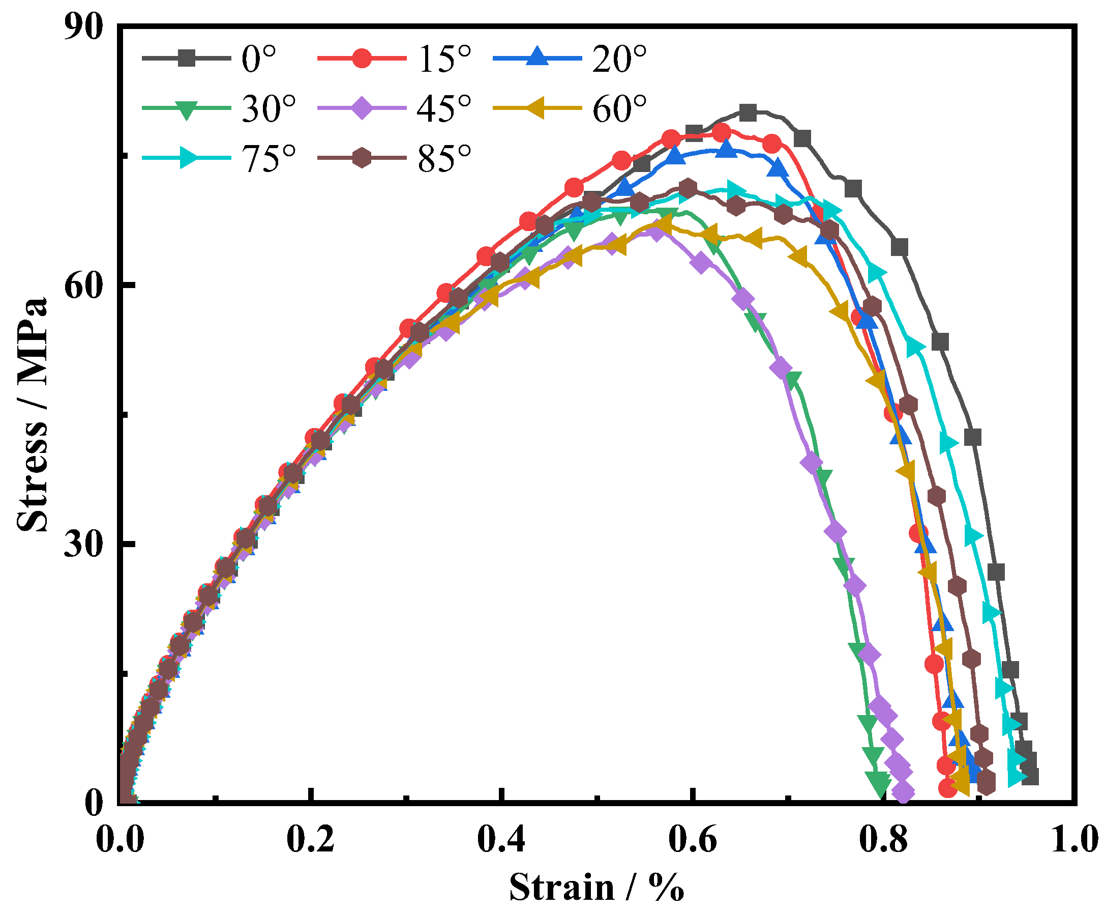
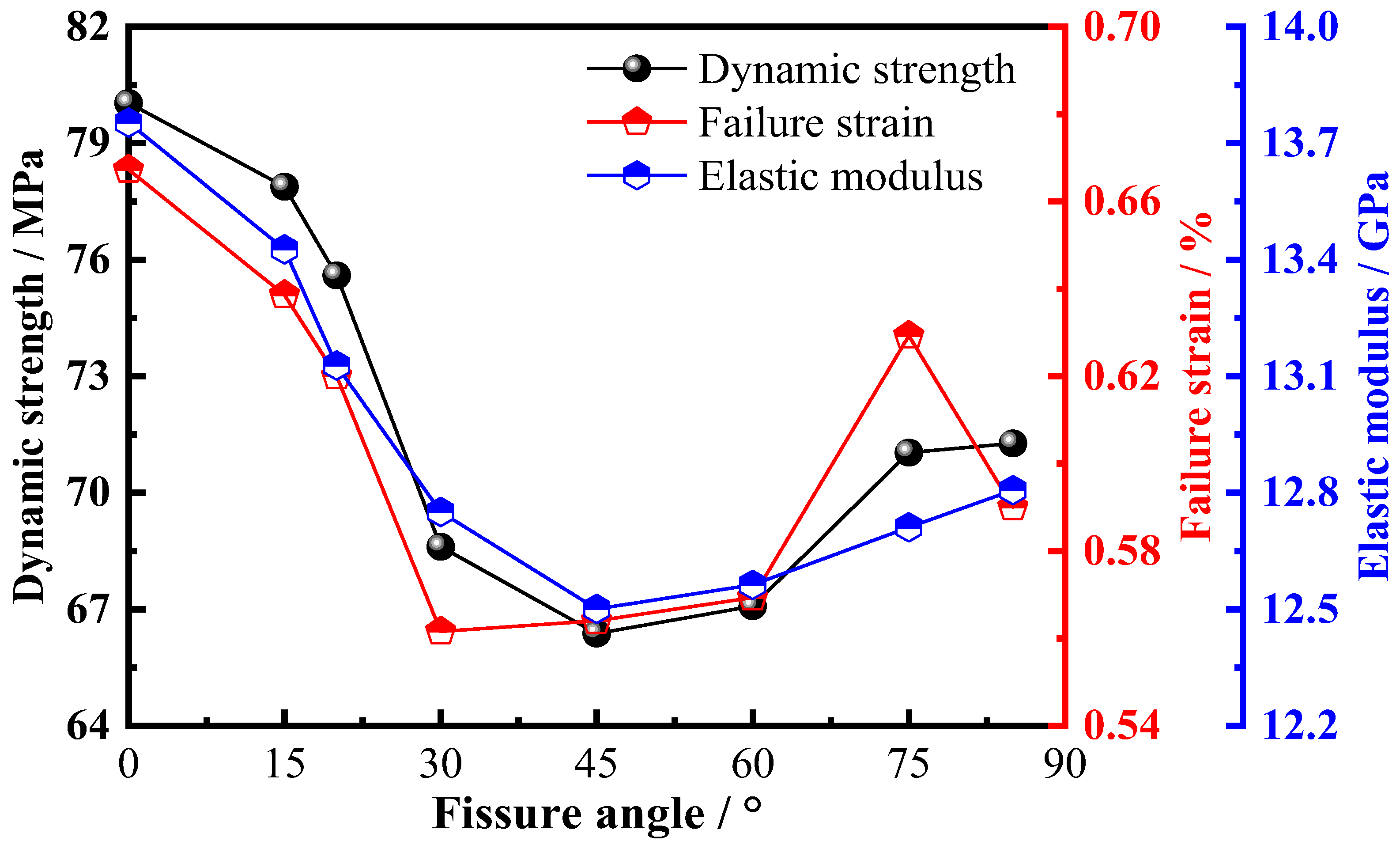
3.1. Dynamic Mechanical Properties of Anchored Bodies at Different Fissure Angles

Figure 11 shows the stress–strain curves of anchored, fissured specimens with different fissure angles from the simulation. It is easy to observe that the curves of the specimens with different fissure angles have similar shapes. Notably, in the initial stage of the simulated curves, the stress increases faster than the strain, and the curve exhibits an “upward convex” shape. After a period of dynamic loading, the curves enter the linear elastic phase with no noticeable densification stage. The differences in the curves at different fissure angles mainly appear in the yielding and the post-peak phases. As the fissure angle increases, the yielding moment of the specimen first increases and then decreases, and the final strain after the peak follows this trend. This indicates an optimal fissure angle under impact loading at which the dynamic mechanical properties of the anchored, fissured specimen are the worst.

To clarify the effect of the fissure angle on the dynamic mechanical parameters of the anchored, fissured specimen, the dynamic strength, failure strain (the strain corresponding to the peak stress), and dynamic elastic modulus, as functions of the fissure angle, were obtained based on the above stress–strain curves, as shown in Figure 12. All three parameters exhibited a general “U-shaped” trend, decreasing initially and then slightly increasing as the fissure angle increased. As the fissure angle increased from 0° to about 45°, the three parameters decreased by 17.08% (dynamic strength), 15.48% (failure strain), and 9.11% (dynamic elastic modulus). This indicates that the dynamic strength is more sensitive to the fissure angle. When the fissure angle exceeded 45°, all three mechanical parameters showed an increase, but the improvement was relatively modest. Specifically, when the fissure angle changed from 45° to 85°, the dynamic strength, failure strain, and dynamic elastic modulus increased by 7.38%, 4.61%, and 2.45%, respectively. This trend likely occurred because at fissure angles near 45°, cracks originating at the tip of the initial fracture are more prone to propagate and extend along the diagonal direction. As a result, the specimen becomes more susceptible to instability and failure at this angle. When the fissure angle exceeds 45°, although the specimen’s load-bearing capacity improves, the anchoring area of the anchor rod in the fracture along the loading direction is reduced, and the anchoring effect is not fully utilized. Furthermore, the closer the fissure angle is to the direction of the anchor rod, the less effective the anchoring effect becomes. Therefore, when the fissure angle exceeds 45°, increasing the fissure angle does not significantly improve the dynamic mechanical properties of the anchored, fissured specimen.

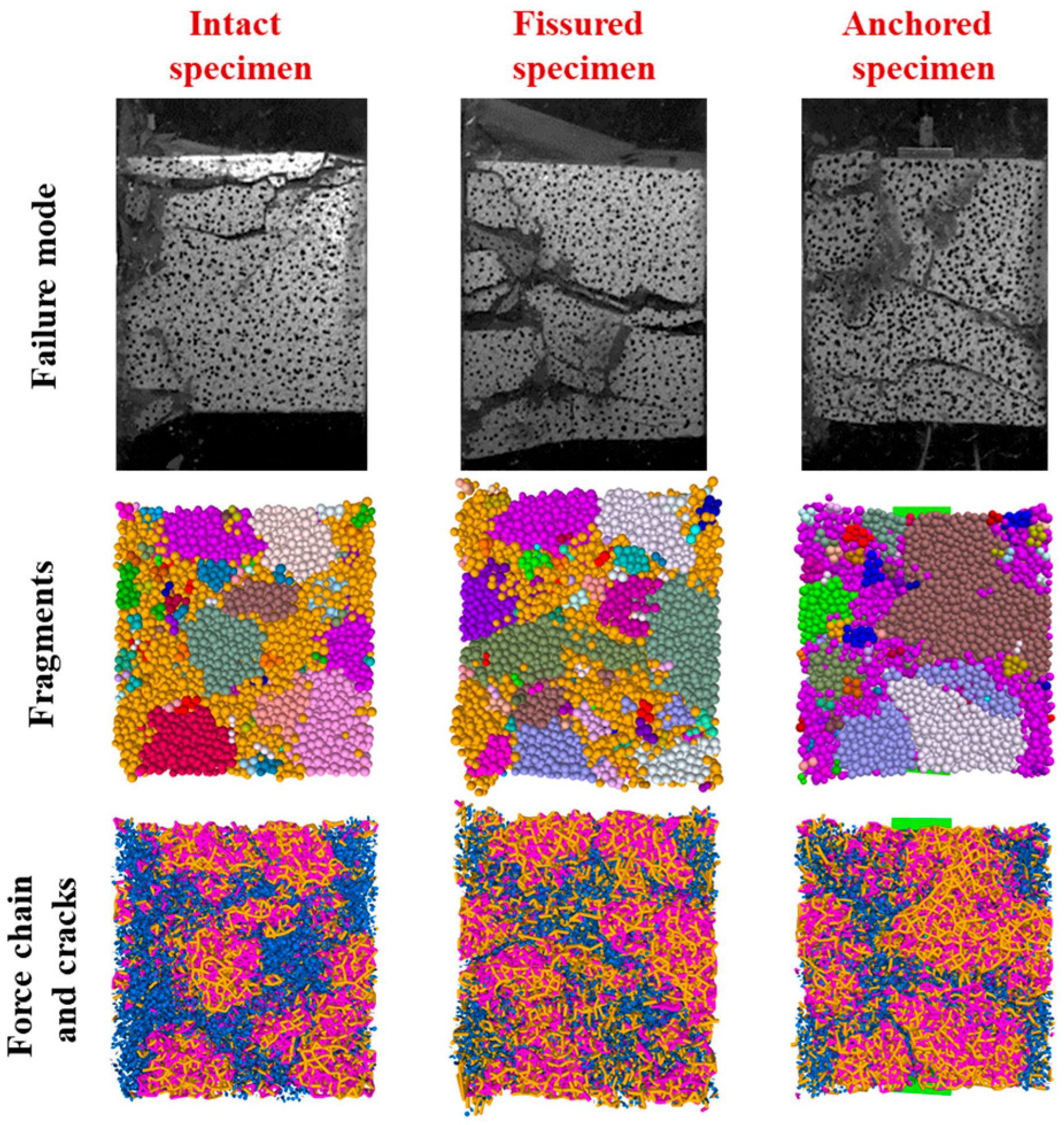
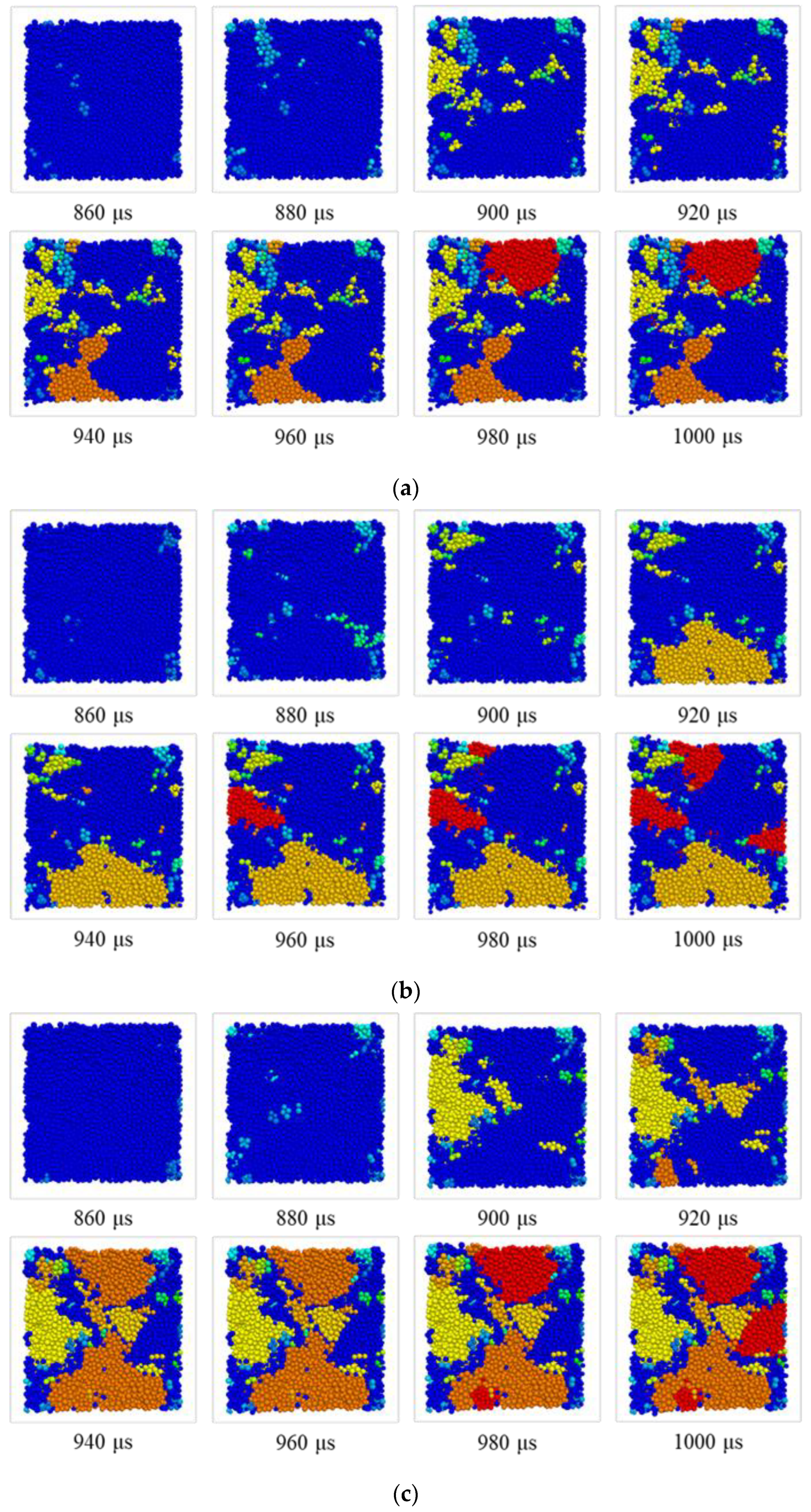
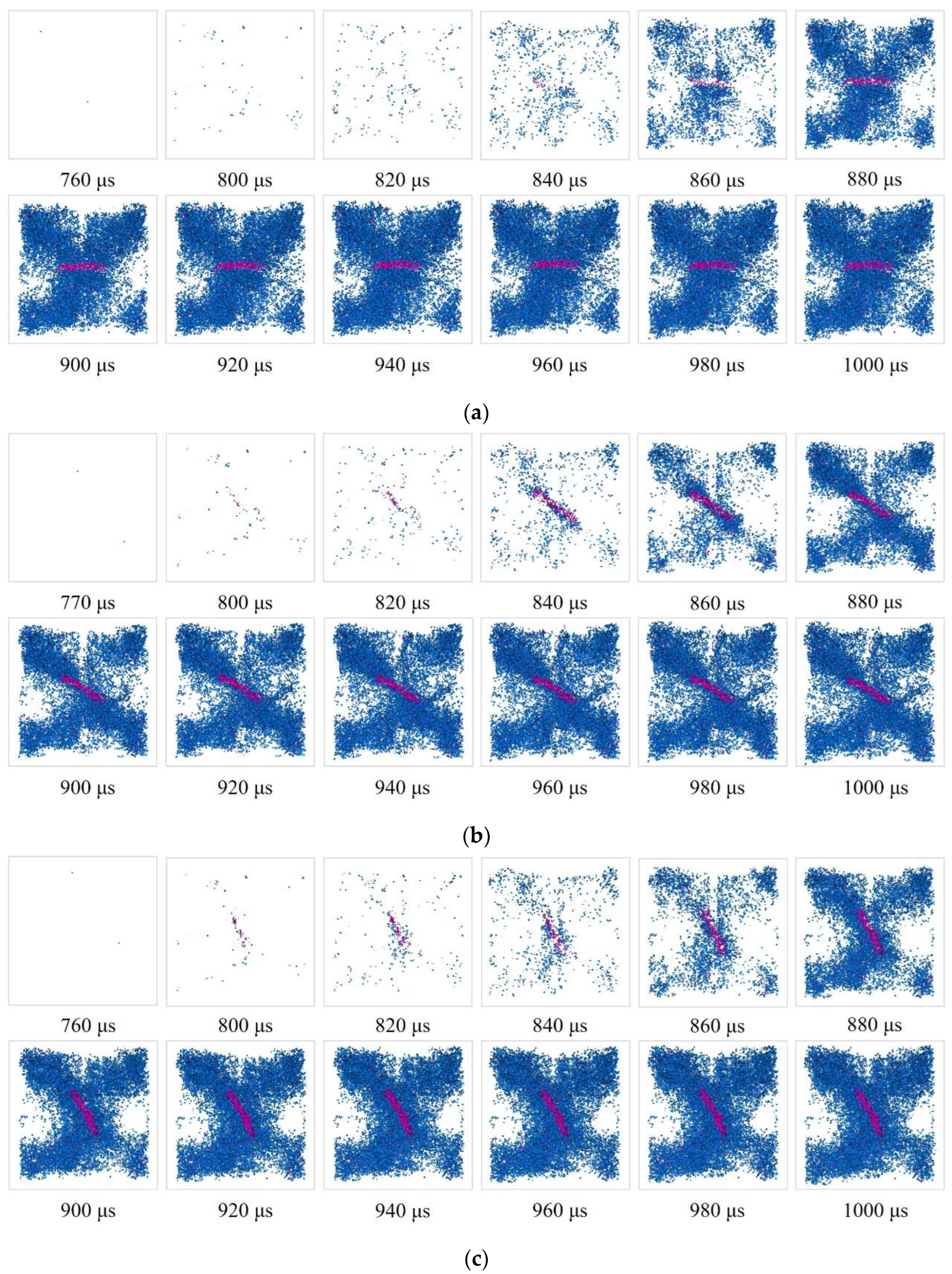
3.2. Fracture Evolution Characteristics of Anchors at Different Fissure Angles

In the particle flow software, the bond between particle contacts fails when its strength surpasses the ultimate strength. This results in crack formation. Therefore, the fracture and fragmentation evolution processes in numerical simulations can be utilized to reveal the fracture evolution characteristics of anchored fissure specimens. Considering the limited length of this article, the evolution processes of cracks and fragments at three fissure angles (0°, 30°, and 60°) were selected for analysis.

Figure 13 and Figure 14 illustrate the evolution of fragments and crack propagation during the dynamic impact failure of the anchored fissure specimen, respectively. The stress–time relationship curve is also shown in Figure 15 to facilitate the analysis of crack and fragment changes. As the duration of dynamic loading increased, the total number of cracks gradually increased and eventually stabilized, fully demonstrating the cracks’ development, initiation, propagation, and through-crack behavior. By combining the results in Figure 14a and Figure 15a, it is evident that cracks initiated at a fissure angle of 0° around 760 μs. At this time, the specimen was still in the linear elastic deformation stage. Afterward, the cracks gradually increased, but the development rate was relatively slow. When the loading duration exceeded 860 μs, the initiation and development of cracks significantly increased, the total number of cracks skyrocketed, and the specimen’s load-bearing capacity gradually decreased. Around 900 μs, the specimen essentially lost its load-bearing capacity, the development of cracks slowed down, and the number of cracks stabilized gradually. As shown in Figure 14a, the cracks were primarily tensile (blue in the figure) and distributed along the diagonal direction. The number of shear cracks (pink in the figure) was relatively small, mainly distributed near the initial fissure. From the distribution of fragments (Figure 13a), we can see that fragments appeared at around 860 μs, near the specimen’s peak stress value. After 980 μs, the fragment distribution remained essentially unchanged, indicating that the specimen had completely fractured. Consequently, the evolution of cracks and fragments served as an effective means of revealing the fracture behavior of the specimen.

The evolution of cracks and fragments at a fissure angle of 30° is illustrated in Figure 13b, Figure 14b and Figure 15b. The overall evolution trend of the number of cracks was generally consistent with that at a fissure angle of 0°, with cracks rapidly appearing after the peak stress value and the rate of increase slowing down after approximately 900 μs. A comparison of crack evolution at 0° and 30° fissure angles showed that cracks near the initial fissure at 30° initiated somewhat earlier. At a fissure angle of 30°, shear cracks (shown in pink) initiated near the initial fissure at around 820 μs. In contrast, at 0°, shear cracks initiated near the initial fissure at around 840 μs. Additionally, at a fissure angle of 30°, the initiation degree of shear cracks near the initial fissure surpassed that of tensile cracks in other regions. In other words, at a fissure angle of 30°, the specimen initially formed primary cracks along the initial fissure, leading to tensile cracks in other regions. This phenomenon also explains why cracks were more likely to develop and initiate along the diagonal direction as the fissure angle approached the diagonal, leading to the degradation of the specimen’s mechanical properties. Regarding fragments, they began to appear at around 860 μs, with the final fracture occurring at approximately 960 μs, which was earlier than at a fissure angle of 0°. Additionally, the distribution of fragments was more regular than at 0°, with fragments forming initially and the final fracture generally following the direction of the initial fissure. At 880 μs in Figure 14b, fragments formed along the lower tip of the initial fissure, and at 1000 μs, the distribution of red and yellow fragments (in Figure 13b) was even more aligned with the direction of the initial fissure. This indicates that the main fracture surface of the specimen exhibited significant angular dependence.

The fracture evolution of the specimen at a fissure angle of 60° is depicted in Figure 13c, Figure 14c and Figure 15c. Similarly to the crack evolution at the other two fissure angles, the cracks gradually increased up to a point near the peak stress value. When the specimen’s strength significantly decreased, the cracks increased sharply. After the specimen’s load-bearing capacity was almost completely degraded, the increase in the cracks slowed down and gradually stabilized. Figure 14 and Figure 15 show that, in comparison with the other two angles, the initiation of cracks near the initial fissure was more pronounced. This suggests that increasing the fissure angle intensified the initial fissure’s influence on the specimen’s cracking behavior. Additionally, the stress–time curve in Figure 15c shows a distinct yielding stage at around 800 μs, indirectly reflecting a more pronounced development of the initial cracks at this angle. Regarding fragment evolution, the distribution of fragments at this angle was also affected by the fissure angle, with fragments forming along the direction of the initial fissure. Meanwhile, the final fracture moment of the fragments occurred at approximately 940 μs, whereas at fissure angles of 0° and 30°, the final fracture moments occurred at approximately 980 and 960 μs, respectively. This indicates that increasing the fissure angle also caused the fracture moment of the specimen to occur earlier.

3.3. Force and Deformation Behavior of Anchors at Different Fissure Angles

The pre-tension force at both ends of the anchor was monitored during the dynamic impact process to analyze the force situation of the anchor. Figure 16 illustrates the variation in the anchor’s pre-tension force with time at fissure angles of 0°, 30°, and 60°. The initial pre-tension force at all three angles was around 2.5 kN, confirming that the initial pre-tension force had been successfully applied to the anchor. Before 600 μs, the stress wave had not yet reached the specimen, and the pre-tension force on both sides of the anchor remained constant. After 600 μs, the pre-tension force of the anchor gradually increased over time, but the increase was not substantial. After approximately 820 μs, the pre-tension force of the anchor increased significantly under all conditions. At this point, the anchor started to participate in load-bearing and exert its anchoring effect. This indicates that the rock-like matrix primarily bears the external load in the early stage of dynamic loading. When the specimen’s load-bearing capacity approached its limit, the anchor’s anchoring and tray constraint effects were activated, causing a rapid increase in the pre-tension force. After the specimen’s strength significantly decreased and fractured fragments formed, the stress between the tray and the specimen was relieved, and the pre-tension force of the anchor gradually diminished. The variation trends of the anchor’s pre-tension force at the three fissure angles were generally consistent, but there were differences in the moments when the pre-tension force became significant. At a fissure angle of 0°, the pre-tension force increased significantly at 820 μs, corresponding to 86.90% of the peak stress moment; at 30°, the significant increase occurred at 825 μs, corresponding to 98.70% of the peak stress moment; and at 60°, the significant increase occurred at 825 μs, corresponding to 95.80% of the peak stress moment. It is evident that the moment when the anchor significantly exerts its effect is influenced by the fissure angle.

To illustrate the stress distribution of the anchor at different moments, Figure 17 presents the stress contour plots of the anchor along the vertical direction at various times for a fissure angle of 30°. As the dynamic loading time increased, the stress distribution of the anchor in the vertical direction generally showed a trend of increasing and then decreasing. At 770 μs, the overall stress distribution of the anchor was relatively low, with localized regions experiencing compressive stress. After 840 μs, the tensile and compressive stresses gradually increased in the middle of the anchor. By 920 μs, the tensile stress and the distribution area reached their maximum, indicating that the anchor had experienced significant tensile loading. At 960 μs, the original tensile stress area of the anchor disappeared, and the compressive stress decreased accordingly, suggesting that the anchor’s deformation had been restored.

Figure 18 distinctly illustrates the force and deformation of the anchor at the moment of the maximum pre-tension force (around 920 μs) under a 30° fissure angle. From the front view, it can be observed that at the point of the maximum pre-tension force, several regions of the anchor showed stress concentration. These regions were aligned with the direction of dynamic loading (x-direction). These significant stress concentration effects led to tensile deformation in localized regions of the anchor, as indicated by the arrows in the figure. In the upper region, the left side of the anchor was under tension while the right side was under compression, causing the anchor’s body to move to the right. In the lower region, the opposite phenomenon occurred, with compressive stress on the left side and tensile stress on the right side, causing the anchor’s body to move to the left. The strain regions highlighted in the figure further demonstrate this phenomenon.

4. Conclusions

This work developed a dynamic loading model for the anchored, fissured surrounding rock body unit based on the coupled finite difference–discrete element numerical method. The impact of the fissure angle on the dynamic response characteristics of the anchored, fissured rock mass was discussed from the perspectives of the dynamic mechanical properties, failure evolution characteristics, and anchor force and deformation behavior. The main conclusions are as follows:

(1)

As the fissure angle increases, the anchored, fissured specimen’s dynamic strength, failure strain, and dynamic elastic modulus generally decrease and then increase, with 45° being the critical angle. However, due to the influence of the anchor placement, the improvement effect is limited. Compared to 0°, at a fissure angle of 45°, the dynamic strength, failure strain, and dynamic elastic modulus decreased by 17.08%, 15.48%, and 9.11%, respectively.

(2)

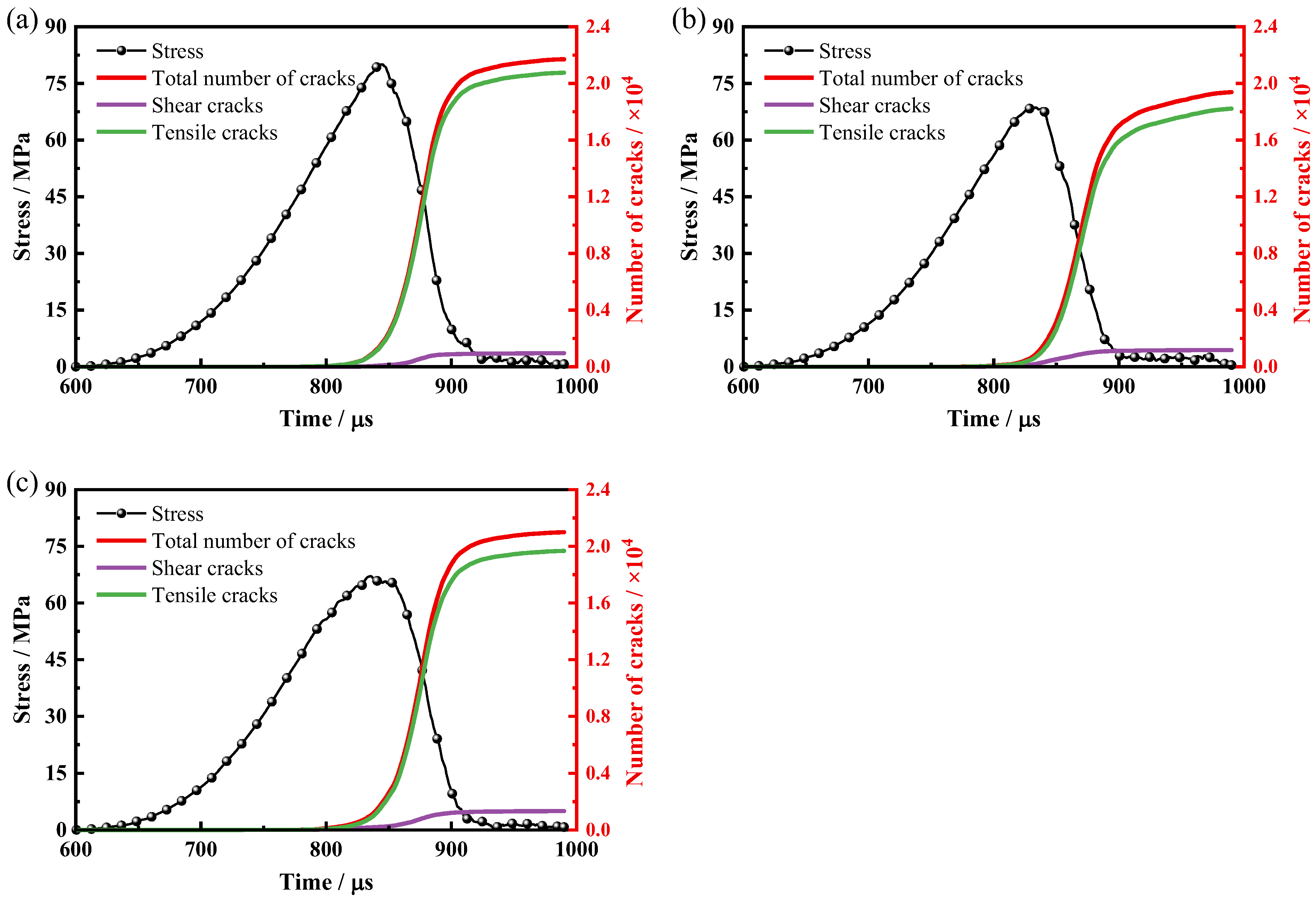
The crack and fragment evolution indicates that as the fissure angle increases, the specimen is more prone to initiating cracks along the direction of the initial fracture. This subsequently leads to the formation of tensile cracks in other areas. Increasing the fissure angle causes the specimen’s final failure time to be earlier and makes the main fracture plane more directional.

(3)

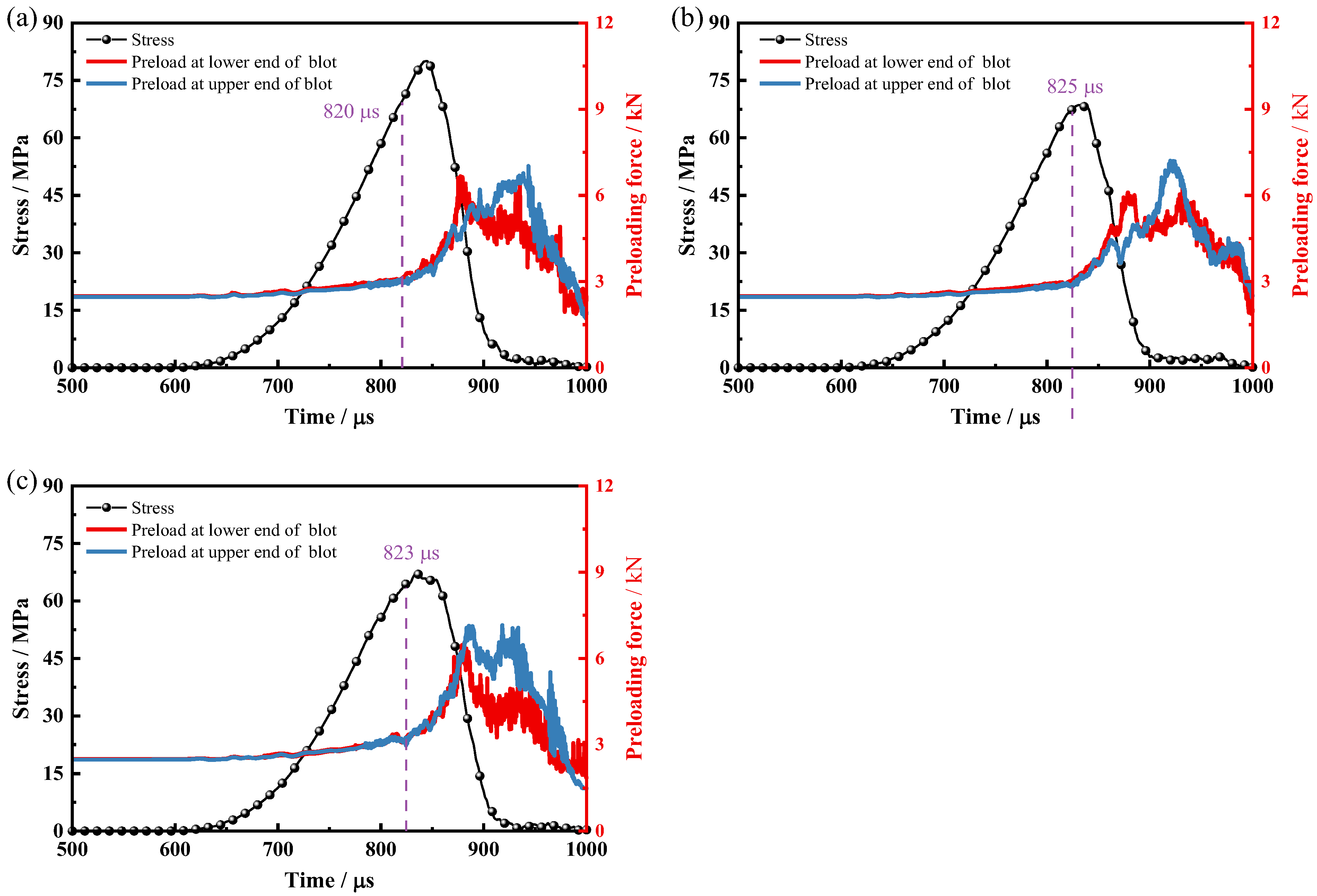
In the early stage of dynamic loading, the pre-tension force of the anchor increases slowly. As the specimen approaches its load-bearing limit, the anchoring and constraint effects of the anchor and tray are effectively activated, and the pre-tension force increases rapidly. After the specimen’s strength significantly decreases, the stress between the tray and the specimen is released, and the pre-tension force gradually decreases. Additionally, the moment at which the anchor exerts its effect is significantly influenced by the fissure angle. The moments of the significant pre-tension force increase for 0°, 30°, and 60° corresponded to 86.90%, 98.70%, and 95.80% of the peak stress, respectively.

References

1. Yang, F.; Zhang, C.; Zhou, H.; Liu, N.; Zhang, Y.; Azhar, M.U.; Dai, F. The Long-Term Safety of a Deeply Buried Soft Rock Tunnel Lining under inside-to-Outside Seepage Conditions. Tunn. Undergr. Space Technol. 2017, 67, 132–146. [Google Scholar] [CrossRef]
2. Zhu, H.; Yan, J.; Liang, W. Challenges and Development Prospects of Ultra-Long and Ultra-Deep Mountain Tunnels. Engineering 2019, 5, 384–392. [Google Scholar] [CrossRef]
3. Das, R.; Singh, T.N. Effect of Rock Bolt Support Mechanism on Tunnel Deformation in Jointed Rockmass: A Numerical Approach. Undergr. Space 2021, 6, 409–420. [Google Scholar] [CrossRef]
4. Zhang, K.; Zhang, G.; Hou, R.; Wu, Y.; Zhou, H. Stress Evolution in Roadway Rock Bolts during Mining in a Fully Mechanized Longwall Face, and an Evaluation of Rock Bolt Support Design. Rock Mech. Rock Eng. 2014, 48, 333–344. [Google Scholar] [CrossRef]
5. Kang, H.; Yang, J.; Gao, F.; Li, J. Experimental Study on the Mechanical Behavior of Rock Bolts Subjected to Complex Static and Dynamic Loads. Rock Mech. Rock Eng. 2020, 53, 4993–5004. [Google Scholar] [CrossRef]
6. Zhang, B.; Li, S.; Xia, K.; Yang, X.; Zhang, D.; Wang, S.; Zhu, J. Reinforcement of Rock Mass with Cross-Flaws Using Rock Bolt. Tunn. Undergr. Space Technol. 2016, 51, 346–353. [Google Scholar] [CrossRef]
7. Yang, S.-Q.; Chen, M.; Tao, Y. Experimental Study on Anchorage Mechanical Behavior and Surface Cracking Characteristics of a Non-Persistent Jointed Rock Mass. Rock Mech. Rock Eng. 2021, 54, 1193–1221. [Google Scholar] [CrossRef]
8. Zhao, T.; Zhang, P.; Guo, W.; Gong, X.; Wang, C.; Chen, Y. Controlling Roof with Potential Rock Burst Risk through Different Pre-Crack Length: Mechanism and Effect Research. J. Cent. South Univ. 2022, 29, 3706–3719. [Google Scholar] [CrossRef]
9. Liu, D.; Chen, H.; Su, R.K.L.; Chen, L.; Liang, K. Influence of Initial Crack Length on Fracture Properties of Limestone Using DIC Technique. Constr. Build. Mater. 2023, 403, 133020. [Google Scholar] [CrossRef]
10. Wang, G.; Liu, T.; Wang, C.; Jiang, Y.; Wu, X.; Zhang, H.; Kong, B.; Zheng, C.; Zhang, Y. Experimental and Numerical Study on the Shear Behaviour of Standard JRC Double-Joint Rock Masses. Int. J. Rock Mech. Min. Sci. 2024, 183, 105930. [Google Scholar] [CrossRef]
11. Peng, Y.; Gao, Y.; Xie, Y.; Zhou, Y.; Wu, T.; Shi, W.; Dong, J. Experimental Study on Instability Failure of Rock Mass with Rough Joints under One-Side Constraint Compression. Theor. Appl. Fract. Mech. 2023, 125, 103907. [Google Scholar] [CrossRef]
12. Baud, P.; Wong, T.; Zhu, W. Effects of Porosity and Crack Density on the Compressive Strength of Rocks. Int. J. Rock Mech. Min. Sci. 2014, 67, 202–211. [Google Scholar] [CrossRef]
13. Zhang, K.; Chen, Y.; Fan, W.; Liu, X.; Luan, H.; Xie, J. Influence of Intermittent Artificial Crack Density on Shear Fracturing and Fractal Behavior of Rock Bridges: Experimental and Numerical Studies. Rock Mech. Rock Eng. 2019, 53, 553–568. [Google Scholar] [CrossRef]
14. Wang, Y.; Deng, H.; Deng, Y.; Chen, K.; He, J. Study on Crack Dynamic Evolution and Damage-Fracture Mechanism of Rock with Pre-Existing Cracks Based on Acoustic Emission Location. J. Pet. Sci. Eng. 2021, 201, 108420. [Google Scholar] [CrossRef]
15. Xia, B.; Li, Y.; Hu, H.; Luo, Y.; Peng, J. Effect of Crack Angle on Mechanical Behaviors and Damage Evolution Characteristics of Sandstone under Uniaxial Compression. Rock Mech. Rock Eng. 2022, 55, 6567–6582. [Google Scholar] [CrossRef]
16. Peng, K.; Wang, Y.; Zou, Q.; Liu, Z.; Mou, J. Effect of Crack Angles on Energy Characteristics of Sandstones under a Complex Stress Path. Eng. Fract. Mech. 2019, 218, 106577. [Google Scholar] [CrossRef]
17. Liu, L.; Li, H.; Zhang, G.; Fu, S. Dynamic Strength and Full-Field Cracking Behaviours of Pre-Cracked Rocks under Impact Loads. Int. J. Mech. Sci. 2024, 268, 109049. [Google Scholar] [CrossRef]
18. Yan, Z.; Dai, F.; Zhu, J.; Xu, Y. Dynamic Cracking Behaviors and Energy Evolution of Multi-Flawed Rocks under Static Pre-Compression. Rock Mech. Rock Eng. 2021, 54, 5117–5139. [Google Scholar] [CrossRef]
19. Sun, X.; Wang, L.; Jiang, M.; Miao, C.; Zhang, Y.; Li, B. Experimental and Numerical Study on the Mechanical Behavior of Layered Rock Anchored by CRLD Anchor Cable. Eng. Fail. Anal. 2024, 165, 108773. [Google Scholar] [CrossRef]
20. Guanping, W.; Jianhua, H.; Jie, W.; Dongjie, Y.; Rui, X. Characteristics of Stress, Crack Evolution, and Energy Conversion of Anchored Granite Containing Two Preexisting Fissures under Uniaxial Compression. Bull. Eng. Geol. Environ. 2022, 82, 5. [Google Scholar] [CrossRef]
21. Chen, Y.; Yu, D.; Wang, Y.; Zhao, Y.; Yang, H.; Huang, L. Dynamic Characteristics and Anchorage Mechanisms of Fractured Granite: Analytical, Numerical and Experimental Analyses. Rock Mech. Rock Eng. 2024, 58, 1569–1589. [Google Scholar] [CrossRef]
22. Fan, D.; Liu, X.; Tan, Y.; Li, X.; Yang, S. Energy Mechanism of Bolt Supporting Effect to Fissured Rock under Static and Dynamic Loads in Deep Coal Mines. Int. J. Min. Sci. Technol. 2024, 34, 371–384. [Google Scholar] [CrossRef]
23. Pothana, P.; Ling, K.; Garcia, F.E. Deformation and Damage Evolution Characteristics in Laminated Rocks Using Discrete Element Method. In Proceedings of the 58th U.S. Rock Mechanics/Geomechanics Symposium, Golden, CO, USA, 23 June 2024; p. D022S022R009. [Google Scholar]
24. Pothana, P.; Garcia, F.E.; Ling, K. Effective Elastic Properties and Micro-Mechanical Damage Evolution of Composite Granular Rocks: Insights from Particulate Discrete Element Modelling. Rock Mech. Rock Eng. 2024, 57, 6567–6611. [Google Scholar] [CrossRef]
25. Ma, Z.; Liao, H.; Dang, F. Unified Elastoplastic Finite Difference and Its Application. Appl. Math. Mech. 2013, 34, 457–474. [Google Scholar] [CrossRef]
26. Procházka, P.P. Application of Discrete Element Methods to Fracture Mechanics of Rock Bursts. Eng. Fract. Mech. 2004, 71, 601–618. [Google Scholar] [CrossRef]
27. Feng, Z.; Lo, C.-M.; Lin, Q.-F. The Characteristics of the Seismic Signals Induced by Landslides Using a Coupling of Discrete Element and Finite Difference Methods. Landslides 2016, 14, 661–674. [Google Scholar] [CrossRef]
28. Huang, F.; Shi, X.; Wu, C.; Dong, G.; Liu, X.; Zheng, A. Stability Analysis of Tunnel under Coal Seam Goaf: Numerical and Physical Modeling. Undergr. Space 2023, 11, 246–261. [Google Scholar] [CrossRef]
29. He, Y.; Zhang, M.; Li, M.; Min, Q.; Deng, G.; Wang, Y. Rolling Simulation and Uneven Stratification Analysis of Electrically Conductive Roller-Compacted Concrete by Coupling Continuous-Discontinuous Method. Constr. Build. Mater. 2024, 419, 135447. [Google Scholar] [CrossRef]
30. Bai, Y.; Li, X.; Yang, W.; Xu, Z.; Lv, M. Multiscale Analysis of Tunnel Surrounding Rock Disturbance: A PFC3D-FLAC3D Coupling Algorithm with the Overlapping Domain Method. Comput. Geotech. 2022, 147, 104752. [Google Scholar] [CrossRef]
31. Zhu, W.; Wang, F.; Mu, J.; Yin, D.; Lu, L.; Chen, Z. Numerical Simulation of Strength and Failure Analysis of Heterogeneous Sandstone under Different Loading Rates. Sci. Rep. 2023, 13, 22722. [Google Scholar] [CrossRef]
32. Zhou, J.; Zhang, L.; Pan, Z.; Han, Z. Numerical Studies of Interactions between Hydraulic and Natural Fractures by Smooth Joint Model. J. Nat. Gas Sci. Eng. 2017, 46, 592–602. [Google Scholar] [CrossRef]
33. He, P.; Kulatilake, P.H.S.W.; Yang, X.; Liu, D.; He, M. Detailed Comparison of Nine Intact Rock Failure Criteria Using Polyaxial Intact Coal Strength Data Obtained through PFC3D Simulations. Acta Geotech. 2017, 13, 419–445. [Google Scholar] [CrossRef]
34. Wen, S.; Huang, R.; Zhang, C.; Zhao, X. Mechanical Behavior and Failure Mechanism of Composite Layered Rocks under Dynamic Tensile Loading. Int. J. Rock Mech. Min. Sci. 2023, 170, 105533. [Google Scholar] [CrossRef]
35. Luo, Y.; Wang, G.; Li, X.; Liu, T.; Mandal, A.K.; Xu, M.; Xu, K. Analysis of Energy Dissipation and Crack Evolution Law of Sandstone under Impact Load. Int. J. Rock Mech. Min. Sci. 2020, 132, 104359. [Google Scholar] [CrossRef]
36. Feng, P.; Dai, F.; Liu, Y.; Xu, N.; Zhao, T. Effects of strain rate on the mechanical and fracturing behaviors of rock-like specimens containing two unparallel fissures under uniaxial compression. Soil Dyn. Earthq. Eng. 2018, 110, 195–211. [Google Scholar] [CrossRef]
Figure 1. Schematic diagram of anchored fissured surrounding rock tunnel under dynamic load disturbance.
Processes 13 00797 g001
Figure 2. Schematic diagram of an anchored, fissured rock mass element.
Processes 13 00797 g002
Figure 3. The Finite-Discrete coupling method: (a) coupling method; (b) schematic diagram of load transfer at the coupling interface.
Processes 13 00797 g003
Figure 4. SHPB dynamic impact numerical loading model.
Processes 13 00797 g004
Figure 5. Contact constitutive diagram: (a) parallel bond model; (b) smooth joint model.
Processes 13 00797 g005
Figure 6. (a) Displacement and strain contours of the anchor rod during the tensile test process; (b) numerical simulation results of the anchor rod tensile test.
Processes 13 00797 g006
Figure 7. (a) Incident stress curves at different dynamic loading velocities, (b) comparison of incident stress waves between numerical simulation and laboratory tests.
Processes 13 00797 g007
Figure 8. Model reliability verification: (a) axial stress distribution, (b) radial stress distribution, (c) rod-end contact force distribution.
Processes 13 00797 g008
Figure 9. Comparison of stress–strain curves from laboratory tests and numerical simulations for different specimens: (a) intact specimen, (b) fissured specimen, (c) anchored specimen.
Processes 13 00797 g009
Figure 10. Comparison of failure modes between indoor tests and numerical simulations for different types of specimens (note: in third row, yellow represents compression force chains, pink represents tension force chains, and blue represents cracks).
Processes 13 00797 g010
Figure 11. Stress–strain curves of anchored, fissured specimens at different fissure angles.
Processes 13 00797 g011
Figure 12. Variation in mechanical parameters with fissure angle.
Processes 13 00797 g012
Figure 13. Fracture process of anchored fissure specimens at different fissure angles: (a) 0°, (b) 30°, (c) 60° (The separated fragments are distinguished using different colors).
Processes 13 00797 g013
Figure 14. Crack propagation process of anchored fissure specimens at different fissure angles: (a) 0°, (b) 30°, (c) 60° (The blue represents tensile cracks, and the pink represents shear cracks).
Processes 13 00797 g014
Figure 15. Crack growth of anchored fissure specimens at different fissure angles: (a) 0°, (b) 30°, (c) 60°.
Processes 13 00797 g015
Figure 16. Variation in anchor’s pre-tension force with time at typical fissure angles: (a) 0°, (b) 30°, (c) 60°.
Processes 13 00797 g016
Figure 17. Variation in the anchor’s stress with time under a 30° fissure angle condition (side view (along the loading direction)).
Processes 13 00797 g017
Figure 18. Stress and strain contour plots at the moment of the maximum pre-tension force of the anchor under a 30° fissure angle condition (red arrow: compressive deformation trend; blue arrow: tensile deformation trend).
Processes 13 00797 g018