Abstract
Porosity prediction from seismic data is of significance in reservoir property assessment, reservoir architecture delineation, and reservoir model building. However, it is still challenging to use traditional model-driven methodology to characterize carbonate reservoirs because of the highly nonlinear mapping relationship between porosity and elastic properties. To address this issue, this study proposes an advanced spatiotemporal deep learning neural network for porosity prediction, which uses the convolutional neural network (CNN) structure to extract spatial characteristics and the bidirectional gated recurrent unit (BiGRU) network to gather temporal characteristics, guaranteeing that the model accurately captures the spatiotemporal features of well logs and seismic data. This method involves selecting sensitive elastic parameters as inputs, standardizing multiple sample sets, training the spatiotemporal network using logging data, and applying the trained model to seismic elastic attributes. In blind well tests, the CNN–BiGRU model achieves a 54% reduction in the root mean square error and a 6% correlation coefficient improvement, outperforming the baseline models and traditional nonlinear fitting (NLF). The application of the proposed method to seismic data indicates that the model yields a reasonable porosity distribution for tight carbonate reservoirs, proving the strong generalization ability of the proposed model. This method compensates for the limitations of individual deep learning models by simultaneously capturing the spatial and temporal components of data and improving the estimation accuracy, showing considerable promise for accurate reservoir parameter estimation.
1. Introduction
Porosity is an important factor that controls fluid storage and flow capacity [1,2]. Accurately assessing porosity distribution from seismic data is essential for evaluating reservoir quality, establishing a reservoir model, and delineating flow units. The traditional process of predicting porosity consists of inverting seismic data to obtain elastic parameters (such as P- and S-wave velocities and densities) and then transforming these elastic parameters into porosity via rock physics models or statistical relationships derived from laboratory/logging data [1,3].
However, tight carbonate reservoirs are characterized by poor physical properties, complex pore structures, variable mineral components, and strong heterogeneity. These features make the physics between the elastic properties of carbonates and porosity highly intricate and nonlinear [4,5,6,7,8,9]. In addition, the coupling effects of porosity and other physical properties, such as the fractions of mineral components, the fluid content, and the pore aspect ratio, on elastic behaviors and seismic attributes might increase the difficulty of accurately estimating porosity. Therefore, it is challenging to estimate the porosity of tight carbonate reservoirs using traditional method.
Deep learning algorithms are well-suited to handling the nonlinear mapping relationship among variables and provide new possibilities for accurate porosity estimation [10,11]. Owing to their excellent nonlinear mapping and feature extraction abilities, deep learning algorithms have been introduced into the geophysical field for seismic data processing and interpretation, including seismic impedance inversion [12,13,14], pre-stack seismic inversion [15,16,17], S-wave velocity estimation [18,19,20,21], reservoir property prediction [22,23,24,25,26], fluid detection [27,28], lithofacies classification [29,30,31] and seismic data denoising [32,33,34].
In recent years, many researchers have explored the application of the representative deep learning algorithms, CNN and RNN, in predicting porosity from well logs and seismic data. Feng et al. proposed a CNN-based unsupervised deep learning approach to estimate porosity from post-stack seismic data, achieving higher prediction accuracy in field data compared with traditional methods [10]. Das and Mukerji designed two porosity quantification strategies and concluded that the direct estimation of reservoir porosity achieves better performance [35]. Yang et al. compared CNNs and RNNs for porosity prediction using pre-stack seismic gathers as input [36]. The results demonstrated that both neural network models effectively track the variation trend of porosity, with the RNN performing better in regions with dramatic changes. Although there have been significant breakthroughs in the use of standard deep learning algorithms (CNN and RNN) for reservoir porosity inversion, these models can only extract spatial features or time-series features of well logs and seismic data, resulting in reduced prediction precision. Furthermore, the majority of studies focus on single-layer neural networks or standard deep learning methods, which are inadequate for mining the complex nonlinearities hidden in geophysical data. Therefore, sophisticated models are required to extract both spatial and temporal features from the data to make more accurate estimates.
Recently, there has been increased interest in the CNN–BiGRU. It combines a CNN to help extract the spatial structures of input data through multilayer convolution [36,37,38,39,40] and a BiGRU, a type of recurrent neural networks (RNNs), to learn long-term temporal dependencies via special gate structures [41,42]. More specifically, the BiGRU model allows for information to be analyzed in both forward and backward directions, which enables the model to capture intricate patterns in the data. In the energy sector, Soares and Franco have applied the CNN–BiGRU neural network to forecast a short-term electric load [43]. In the marine environment, a hybrid CNN–BiGRU, combined with a Bayesian optimization algorithm, has been proposed by Li et al. to predict the sea level changes [44]. In terms of social public service, Wang et al. have demonstrated the superiority of the CNN–BiGRU over other deep learning methods in predicting the service prices of urban charging infrastructure [45]. In earth science, a CNN–BiGRU model with an attention mechanism has been successfully applied to estimate the shear wave velocity and shale content from well logs. However, the application of the CNN–BiGRU model to predict seismic porosity has been rarely reported.
In this study, a hybrid spatiotemporal neural network that combines the strengths of CNN and BiGRU is proposed for porosity prediction. First, the sensitive elastic properties are selected as inputs and normalized before they are fed into the network. Then, the CNN model is used to extract the local features, and the BiGRU is employed to capture the temporal features, guaranteeing that the model accurately expresses the spatiotemporal aspects of the input data. Meanwhile, the fully connected layers are used to establish a nonlinear relationship between the extracted features and the porosity. The prediction accuracy and generalization ability of the new network are compared with CNN, BiGRU, and the traditional NLF method using well logging data. Finally, the presented network is applied to predict the spatial distribution of the porosity in a tight carbonate reservoir in the Ordos Basin, central China.
This aim of this study is to enhance the accuracy of reservoir parameters and provide a reliable tool for reservoir characterization. The structure of this study is organized as follows. First, the CNN–BiGRU-based porosity inversion method is proposed. Then, a brief description of the geological background and dataset used in this study is given. Next, the predictive performance and generalization of the proposed method are verified by blind well testing. Finally, the seismic-derived elastic properties are fed into the trained network to estimate the porosity distribution of the target reservoir.
2. Methodology
2.1. Workflow
Deep learning is considered the most promising method in the field of machine learning, and has been widely used in image analysis, speech recognition and text comprehension. The most widely used deep learning methods are CNNs and LSTM, in which CNNs can strongly extract spatial features, while GRUs, a variant of LSTM, can fully mine temporal features. To take advantage of these methods to accurately predict porosity, it is necessary to combine them to build a new model that can provide their own advantages.
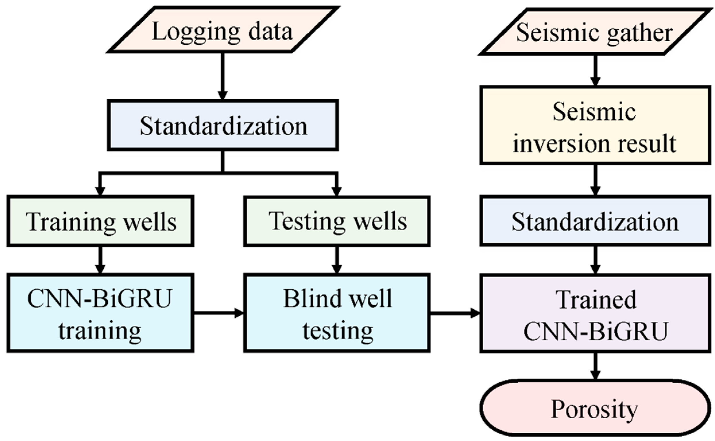
Figure 1 shows the workflow of the method, which includes three main parts: labeled data preparation, deep learning model training and seismic porosity inversion. The detailed steps are as follows:
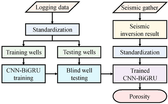
Figure 1.
The workflow of seismic porosity estimation based on a spatiotemporal network.
- (1)
- Preparation of labeled data. Abnormal values (i.e., zero or negative values) are first removed from the porosity logging data. Then, the input logging measurements are standardized to ensure consistent training across different features. Finally, the input data are divided into training and test data.
- (2)
- Deep learning model training. A CNN–BiGRU model is built and trained with the labeled data by adjusting the hyperparameters through multiple iterations. The generalization performance is verified through blind well testing.
- (3)
- Seismic porosity inversion. The trained network model is applied to the pre-stack seismic inversion results to obtain the spatial distribution of porosity.
2.2. CNN for Spatial Feature Extraction
As the most commonly used deep learning algorithm, CNNs has are characterized by sparse interaction and weight sharing, which significantly reduces the complexity of the model. They offer significant advantages in high-dimensional data processing, complex feature mapping, and image processing.
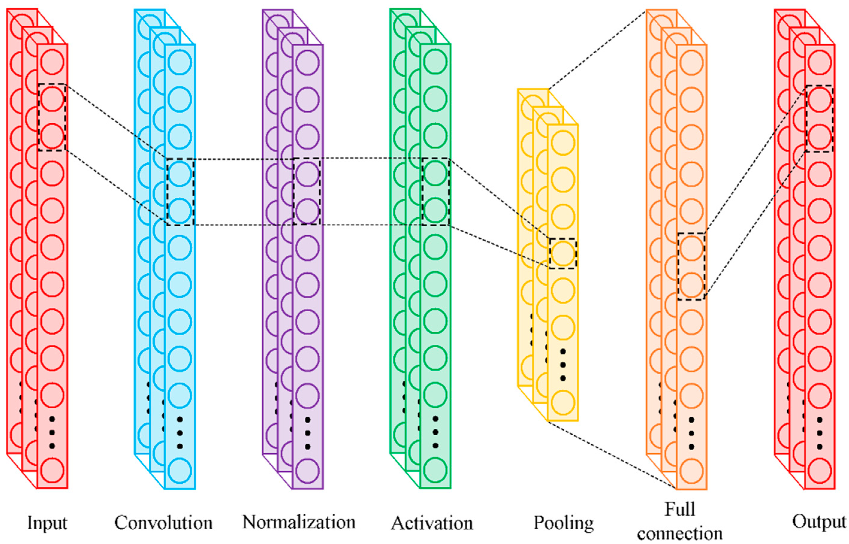
The CNN structure mainly includes convolution, activation, normalization, pooling, and full connection layers (Figure 2). Among them, the convolution layer is composed of a series of filters known as convolutional kernels. Based on these convolutional kernels, a convolution operation can be performed by sliding the convolution kernels with a certain step over the input vector to extract features and reduce the effect of noise [19]. As a feature mapping layer, the pooling layer summaries the characteristics extracted by convolution layers and reduces the dimension of the data through operation such as maximum pooling and average pooling (select the maximum or average value in local input vector as output), which can avert overfitting [46]. The activation layer provides the nonlinear computing power for CNN through various activation functions such as Sigmoid, ReLU and Tanh (they all establish nonlinear relationship between their input and output) [40]. The full connection layer composed of a series of neurons that is connected fully with those in previous layer is utilized to match dimension between convolutional outputs and labeled data [36]. The normalization layer stabilizes the distribution of nonlinear inputs by normalizing the samples within a mini-batch using a scaling factor and a shift factor [47].
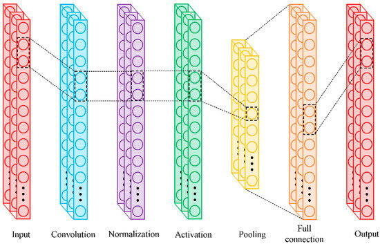
Figure 2.
The architecture of the CNN.
2.3. Bidirectional GRU for Temporal Feature Extraction
RNNs are often used to process time series data. However, RNNs are limited in terms of memory and storage. They cannot learn long-term dependencies well and experience issues with the gradient exploding and vanishing. To overcome these drawbacks, Hochreiter proposed a long short-term memory neural network (LSTM) [48]. As a variant of the RNN, the LSTM controls information extraction by adding an input gate, forget gate and output gate. This gate system enables LSTM to learn over the long term, retaining useful information and forgetting useless information. However, due to the introduction of complex structures, the number of operational parameters rises, which increases the difficulty of training models.
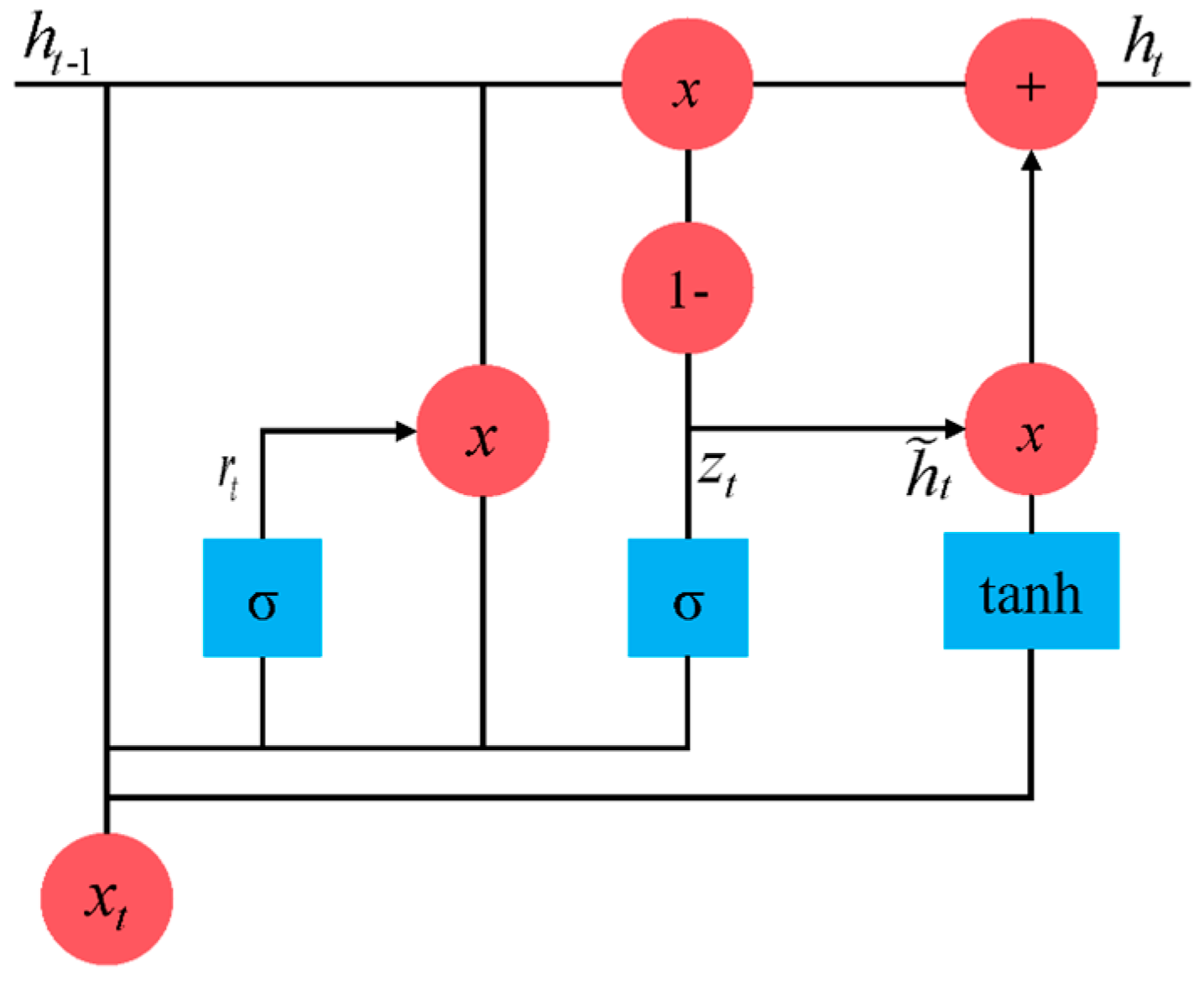
To improve computational efficiency, GRUs are proposed based on LSTM [49]. Compared with LSTM, GRUs simplify the structure by combining the forget and input gates into the update gate and retaining and discarding information via the update and reset gates. Its internal structure is shown in Figure 3, and the calculation procedure [50] is as follows:
where and represent the output of the reset gate and update gate, respectively; and represent the candidate hidden state and hidden state of memory cells in the current moment, respectively; stands for the hidden state of memory cells in the previous moment; , and represent the weight matrices of input data in the reset gate, update gate and calculation of the candidate hidden state, respectively; , and represent the weight matrices of the hidden states in the reset gate, update gate and calculation of the candidate hidden state, respectively; and , and represent the bias vectors in the reset gate, update gate and candidate hidden state calculation, respectively.
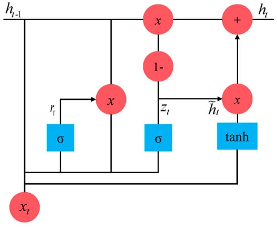
Figure 3.
The internal structure of the GRU network.
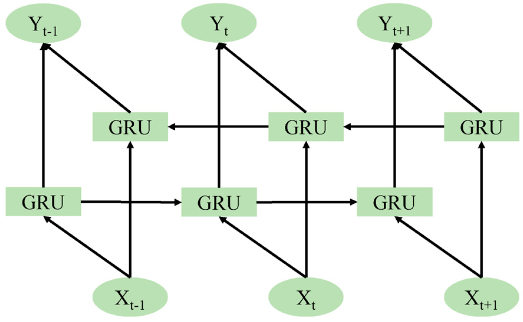
A BiGRU can be regarded as a structure that combines forward and backward propagation GRUs. Therefore, the BiGRU model can learn using historical and future information simultaneously, which overcomes the limitation of unidirectional GRUs. Figure 4 shows the structure of the BiGRU. It can be seen that its output is determined by the linear superposition of the forward propagation hidden layer and the backward propagation hidden layer. When the model is applied to porosity evaluation, the network can utilize the information of the upper and lower reservoir intervals from two directions to predict the current state of the reservoir intervals.
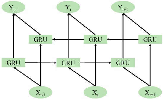
Figure 4.
The structure of the BiGRU network.
2.4. Establishment of the CNN–BiGRU Model
To establish a highly nonlinear mapping relationship between the elastic properties and porosity, a CNN–BiGRU neural network, which makes full use of the local perception ability of CNN and the long-term memory of the BiGRU, is proposed. The network utilizes structural advantages to compensate for the disadvantages of each model, thereby reducing training time, accelerating network convergence, and improving generalization performance. Specifically, a CNN can better learn the intrinsic features of logging and seismic data without causing significant information loss. In addition, logging and seismic data can be regarded as vertically interrelated time series data, and the BiGRU can capture the time series characteristics of these data well. Therefore, CNNs are used to extract features from the input data, and this extracted information is then used as the input of the BiGRU to obtain the output information.
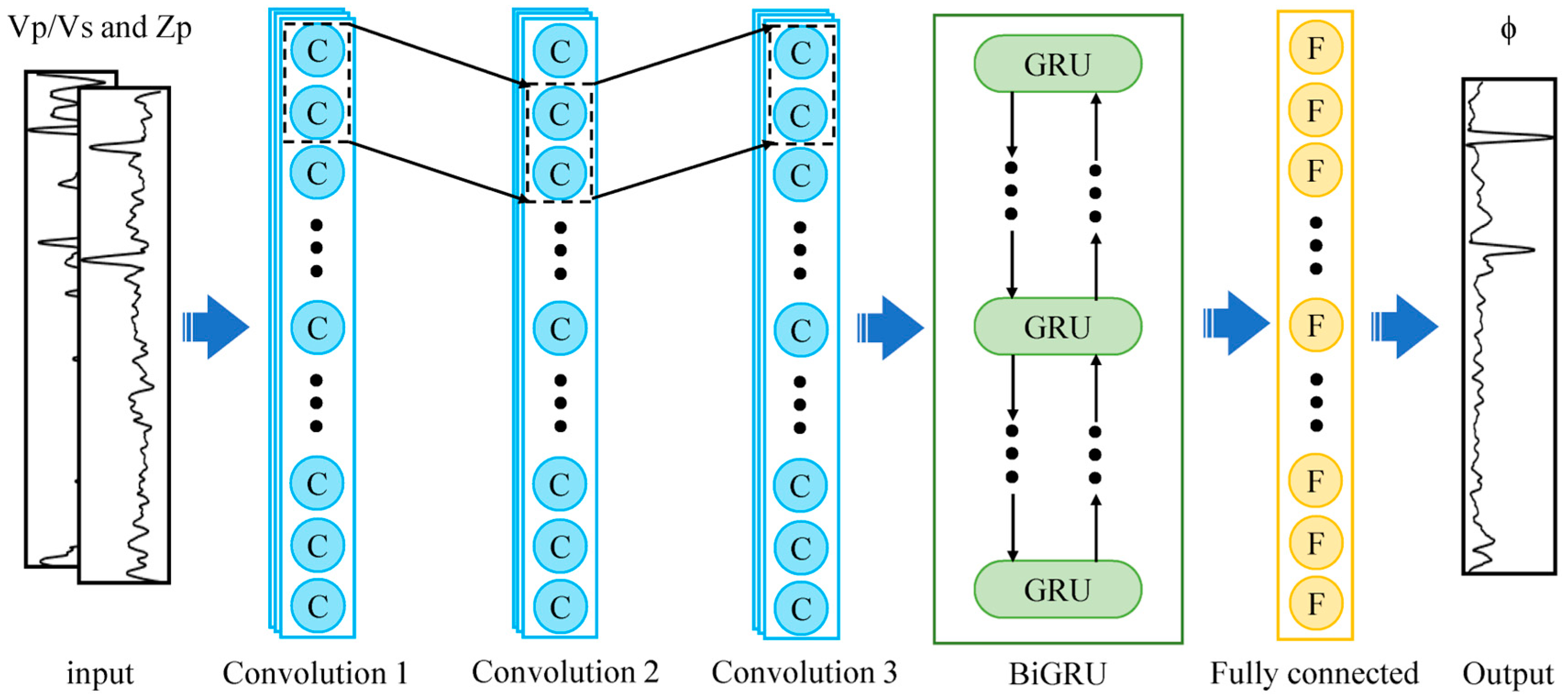
The structure of the CNN–BiGRU model designed in this study is illustrated in Figure 5. The model can be divided into the following three parts: (1) inputting the processed logging data into CNN and extracting the spatial structure features through CNN; (2) taking the output of CNN as the input of the BiGRU and then using the BiGRU to obtain deep-seated time sequence characteristics; (3) using the full connection layer to effectively integrate the special output by the BiGRU.
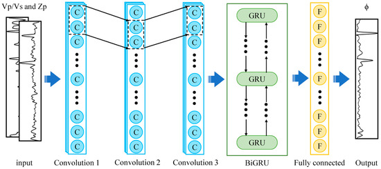
Figure 5.
The workflow of the proposed porosity evaluation strategy is based on the CNN–BiGRU.
2.5. Evaluation Criteria
In this study, two primary metrics, the Pearson correlation coefficient (PCC) and root mean square error (RMSE), are used to assess the performance of the porosity evaluation. The higher the former value or the lower the latter value corresponds, the higher accuracy of the model. The RMSE describes the standard deviation between the model output and actual logs [51]. It can be defined as
where and are time series data, representing the predicted value and the true values, respectively. denotes the number of sampling points.
In contrast, PCC reflects the linear dependence between the model output and real logging measurements [52]. It can be expressed as
where the mean values are represented as and , respectively.
3. Geological Background
The study area is located in the eastern Ordos Basin, northwest of China, and is a significant oil- and gas-bearing basin in China. The sediment in the basin is primarily marine carbonate rock from the later Ordovician to the middle Cambrian. Based on sedimentary characteristics and lithology, the Majiagou Formation can be subdivided into six members. The fourth member and a portion of the fifth member of the Ordovician (Ma 4 and Ma 510) are selected as the interval of interest (Figure 6). The sedimentary environment of the Ma 4 member is mainly a restricted platform, primarily consisting of dolomite and limestone, while the Ma 510 member is mainly an evaporating platform, primarily consisting of gypsum rocks, limestone and dolomite [53]. The study area, located in the Shenmu-Mizhi low uplift in the east of the basin, is significantly influenced by the sedimentary environment, diagenesis and reservoir distribution patterns, resulting in strong heterogeneity and complex pore structures. The reservoir types are dominated by cracks, micropores, vuggy pores, and intercrystalline pores as displayed in Figure 7. These heterogeneous pore structures related to depositional environment and post-depositional diagenesis significantly affect reservoir elastic behaviors and seismic responses, posing great challenges for seismic reservoir characterization.
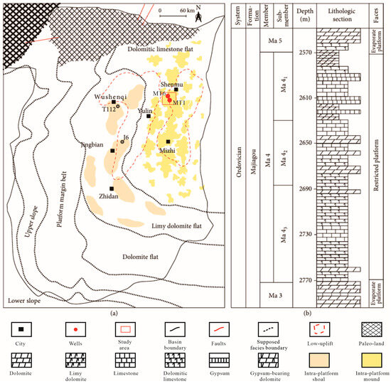
Figure 6.
Paleogeographic map and lithologic sequence stratigraphic column of Ordovician Ma 4 and a portion of the Ma 5 member in the study area. (a) Paleogeographic map. (b) Lithologic and stratigraphic column diagram.

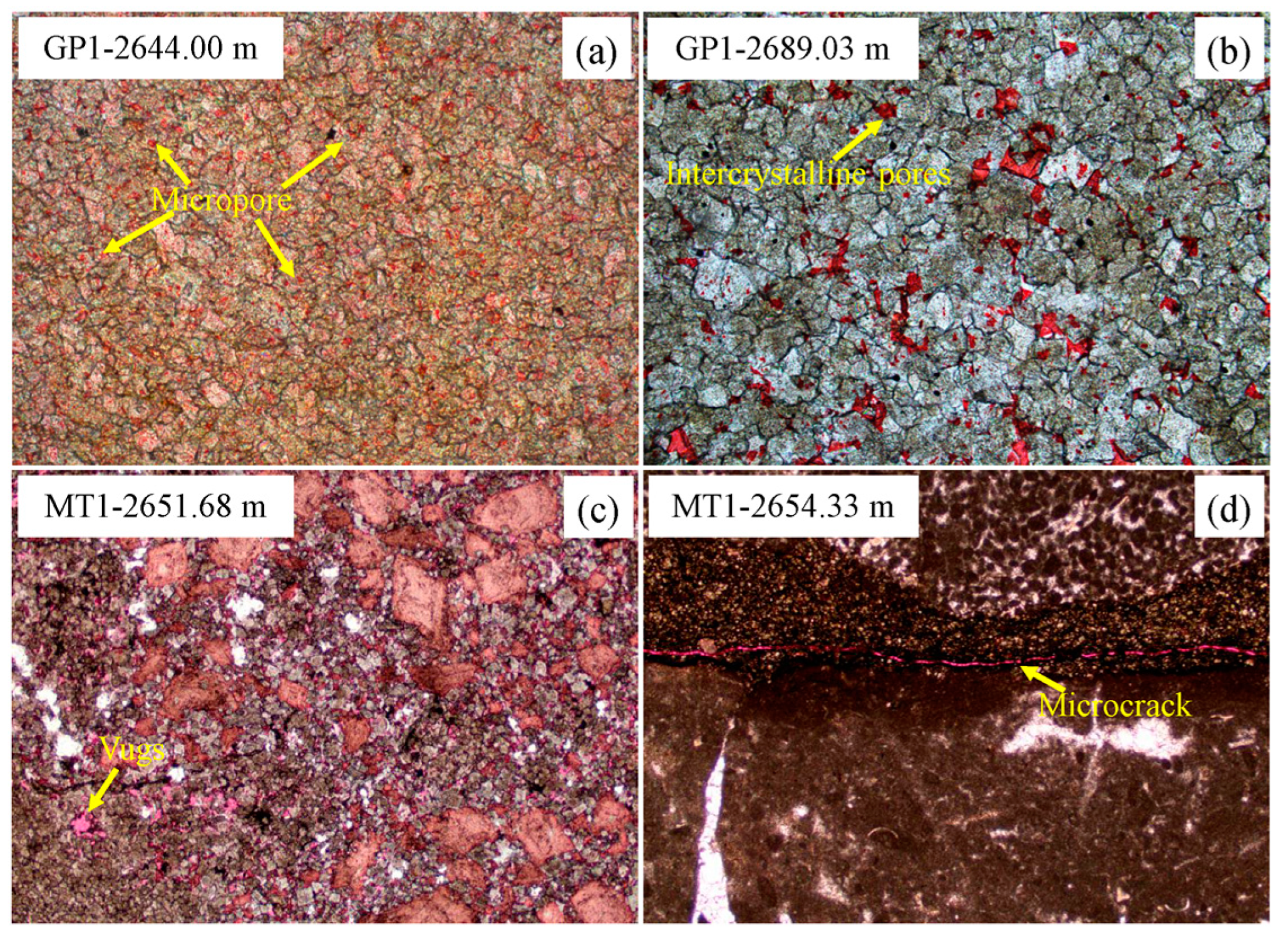
Figure 7.
Thin sections showing pore systems of the Ordovician Majiagou carbonate reservoirs in the Ordos Basin. (a) Micropore, well GP 1; (b) intercrystalline pores, well GP 1; (c) intercrystalline pores and vuggy pores, well MT 1; and (d) microcracks, well MT 1.
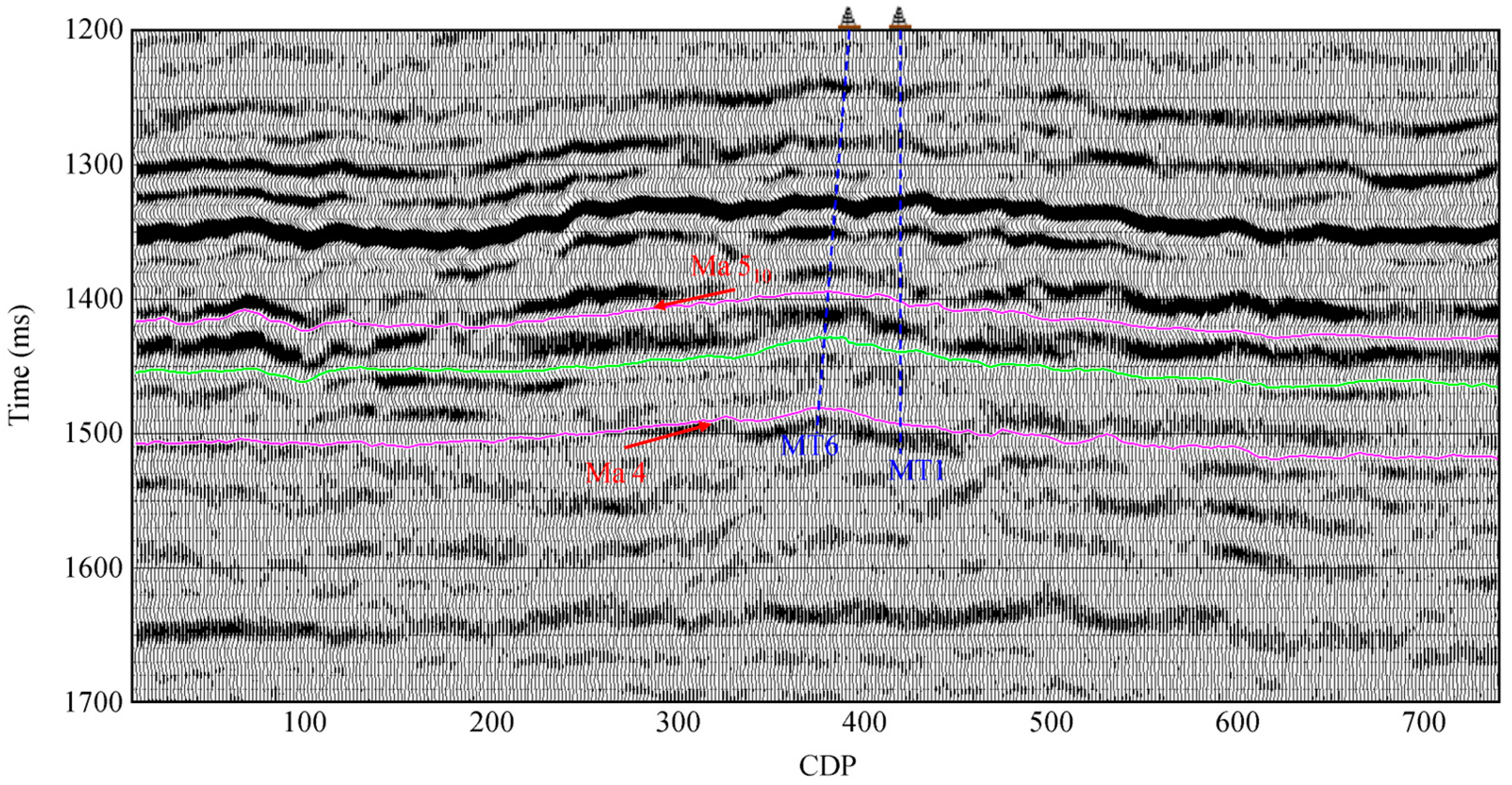
The dataset used in this study includes logging data from five wells (MT 1, MT 6, MT 7, GP 1, and Shen 85) and a 3D seismic cube from the Ordos Basin. Among these data, the logging data from wells MT 6, MT 7, GP 1, and Shen 85 are chosen to train the established spatiotemporal network and the data from well MT 1 are used for blind well testing. Figure 8 illustrates the post-stack seismic profile through wells MT 1 and MT 6, with Ma 4 and Ma 510 selected as target layers ranging from approximately 1390 ms to 1520 ms. In Figure 8, seismic events in the Ma 510 formation exhibit a degree of regularity and continuity, whereas those in the Ma 4 formation appear weak and indistinct. This poor data quality might be associated with the complex pore structure, heterogeneous reservoir properties, and imperfect seismic data processing. The elastic attributes (the P-wave impedance and Vp/Vs ratio) inverted from pre-stack seismic gathers are used as input data for seismic porosity evaluation.
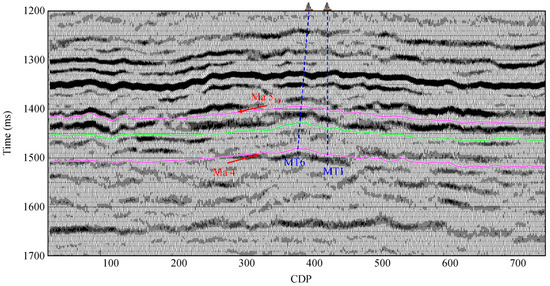
Figure 8.
The post-stack seismic profile through wells MT 1 and MT 6 with the upper layer Ma 510 and the low layer Ma 4 marked in the targeted inversion area.
4. Model Training and Blind Well Testing
4.1. Sensitivity Analysis
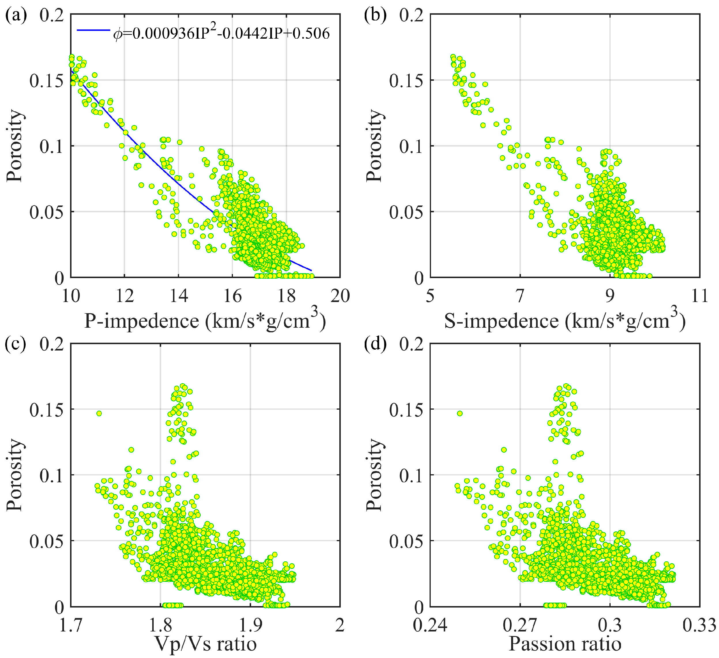
Seismic elastic properties are jointly controlled by many geological factors such as mineral contents, fluid saturation, and porosity. Typically, different porosities may correspond to the same elastic properties. Hence, it is necessary to select the porosity-sensitive elastic parameters as input to reduce the risk of over-fitting and decrease computational costs. Figure 9 shows the cross-plots of porosity versus the P-wave impedance, S-wave impedance, Vp/Vs ratio, and Poisson’s ratio, where the P- and S-wave impedances, Vp/Vs ratio and Poisson’s ratio exhibit a negative correlation with porosity. Although these elastic properties overall decrease with porosity, they can vary significantly for the given porosity. This is likely caused by the heterogeneous pore structures. To compare the proposed deep learning method with the traditional model, a nonlinear fitting relationship between porosity and P-wave impedance () is determined via petrophysical analysis of the logging data. This sensitivity analysis highlights the necessity of using deep learning instead of a model-driven method to predict porosity from the P-wave impedance and Vp/Vs ratio.
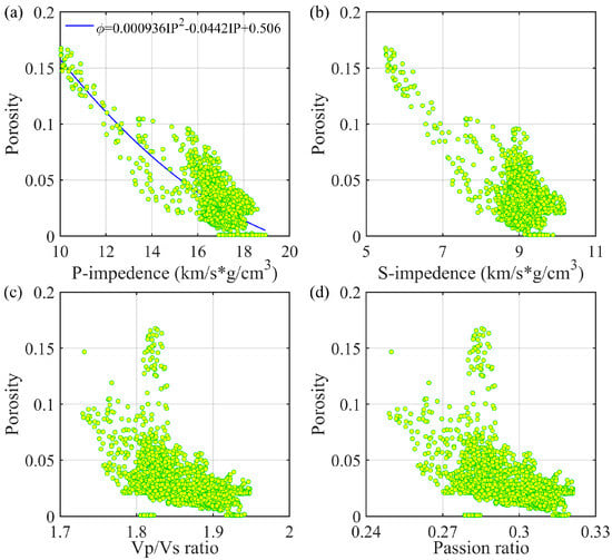
Figure 9.
The cross-plot of P-wave impedance (a), S-wave impedance (b), Vp/Vs ratio (c) and Poisson’s ratio (d) versus porosity.
4.2. Hyperparameter Optimization
The built CNN–BiGRU model consists of three convolution layers, and the number of convolution kernels in each layer is 128. To retain as much feature information extracted by the CNN as possible, the pooling layers are abandoned when designing the network. One BiGRU layer with 48 units in each layer and one full connection layer with one neuron is considered. To avoid over-fitting, a dropout layer is followed by the full connection layer [54], and its parameter is set to 0.2. The total number of epochs is set to 100. The learning rate is a hyperparameter that adjusts the network weight based on the gradient of the loss function. A lower learning rate will increase the complexity of the network, leading to the model being trapped in the local minimum. Conversely, a higher learning rate results in the model failing to converge to the local minimum. Here, the adaptive learning rate attenuation method is adopted, and the initial learning rate is set at 0.001. To minimize the loss function, the Adam algorithm [55] is selected as the optimizer for network training. In real applications, these hyperparameter configurations can be adjusted for better evaluation performance.
4.3. Data Normalization
To eliminate the influence of varying scales during network training, the well-log data should be standardized before feeding to the network. Discrete logging data are normalized to [0, 1] according to the following equation:
where is the standardized value of the ith sample; is the real value of each well-log for all samples; and are the minimum and maximum values of each well-log for all samples.
4.4. Model Training
To evaluate the accuracy and applicability of the model, the data from two wells MT 6 and MT 7 in the study area, and two wells in the adjacent area Shen 85 and GP 1 are used as input data to train the hybrid network and its baseline models, and the remaining well MT 1 is used as blind well test to evaluate the performance of the three models. For each deep learning algorithm except for the NLF method, the input data are the P-wave impedance and Vp/Vs ratio. In contrast, for the NLF method, we build the nonlinear relationship between P-wave impedance and porosity (Figure 9a) to compare the porosity estimates with other methods. Before training the CNN–BiGRU and its baseline models (CNN and BiGRU), the input data are normalized using Equation (7). The datasets from the five wells are divided into two parts: 81% is used for training, and the remainder is used for testing. The testing dataset does not participate in network training. The performance of the trained CNN–BiGRU, CNN and BiGRU models is quantified in terms of the RMSE and PCC.
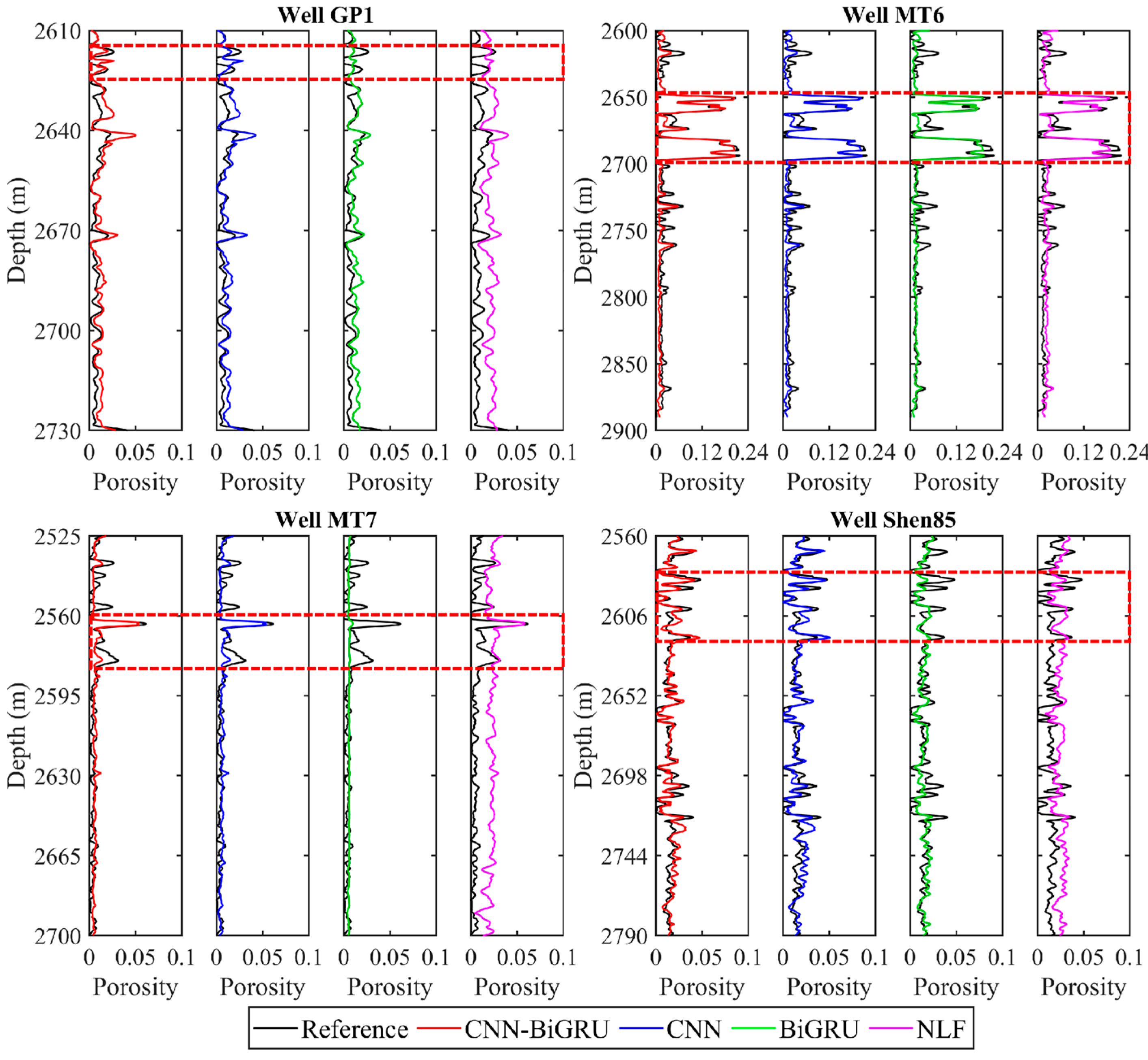
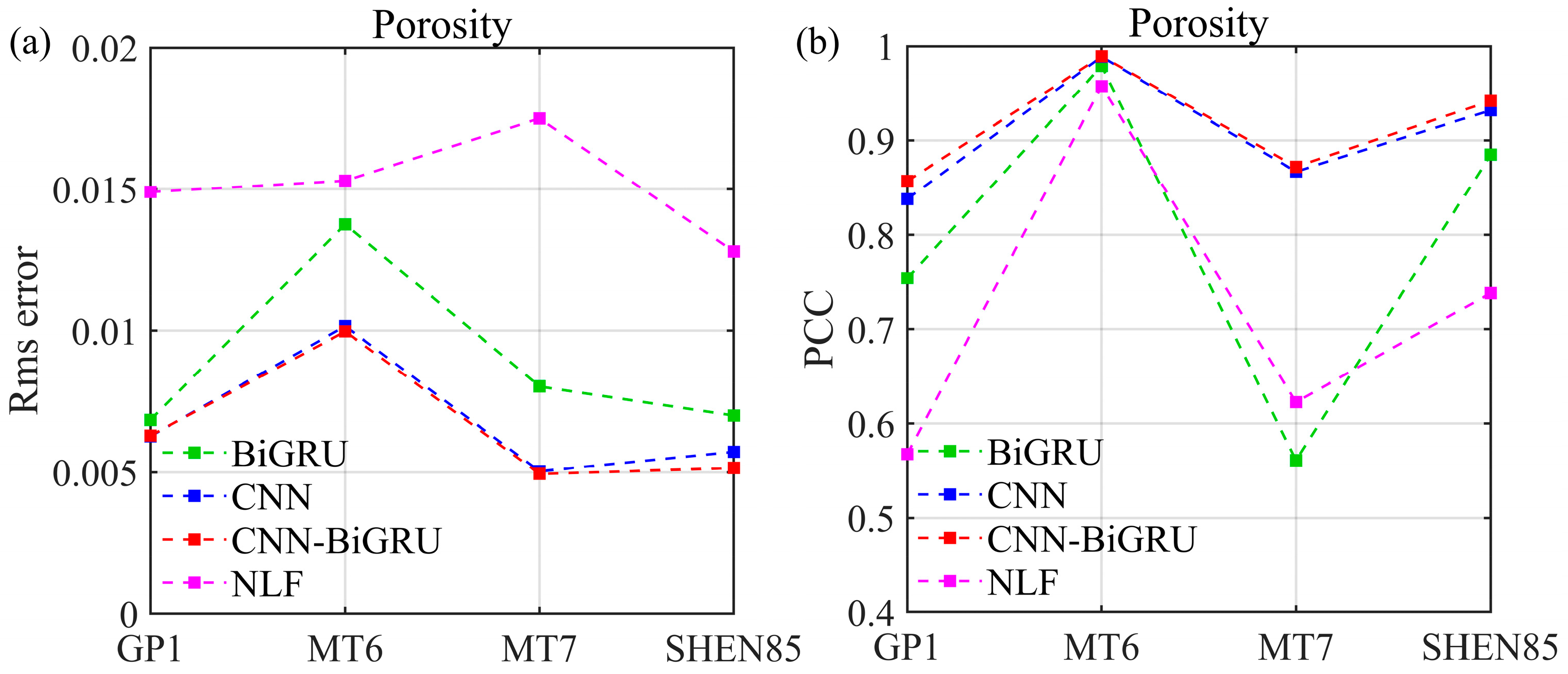
Figure 10 shows the porosity evaluation results from the four training wells using the three network models and one traditional NLF method. As expected, the overall porosity estimates of the CNN–BiGRU model are close to the real porosity and superior to the estimates of the CNN, BiGRU and NLF methods, especially at the depths of 2615–2625 m in well GP 1, 2645–2670 m in well MT 6, 2560–2580 m in well MT 7, and 2582–2628 m in well Shen 85. To compare the predictive accuracy of different models, the RMSE and PCC for each model are calculated for comparison. As shown in Figure 11, the CNN–BiGRU model obtains the smallest RMSE and largest PCC, clearly standing out from the compared CNN, BiGRU, and NLF methods. This is because the CNN–BiGRU model takes into account both spatial and temporal features in logging data, while a single network can only extract one of the two types of information, and the empirical formula makes it difficult to accurately describe the complex nonlinear mapping relationship between the elastic properties and porosity for heterogeneous carbonate reservoirs.
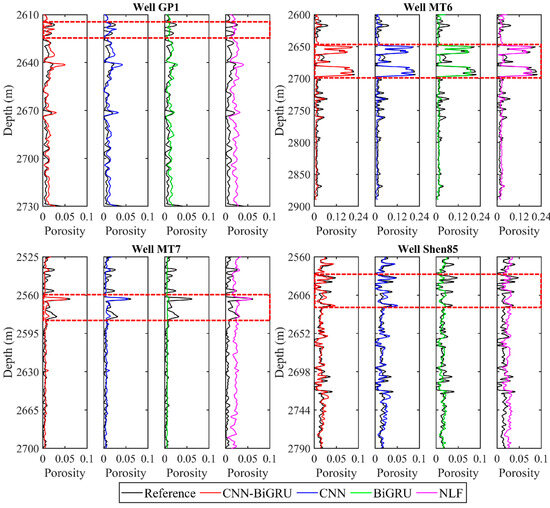
Figure 10.
Evaluation results of wells MT 6, MT 7, Shen 85 and GP 1 using CNN–BiGRU, CNN, BiGRU and NLF methods. All porosities are smoothed with a 35-point running average. The black curves represent the porosity log taken as the reference; the other red, blue, green and pink curves represent the porosities estimated based on CNN–BiGRU, CNN, BiGRU, traditional NLF models, respectively. The dashed red boxes mark some areas where the porosity prediction results have been improved by applying the CNN–BiGRU model.
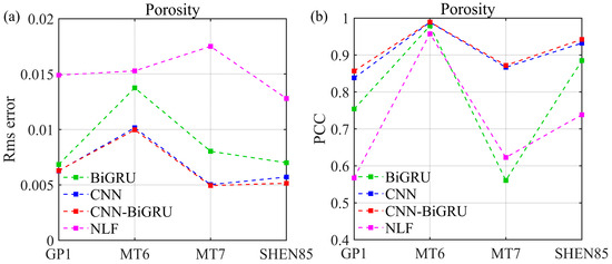
Figure 11.
RMSE (a) and PCC (b) of evaluation results for four training wells. The red, blue, green and pink dash lines represent the RMSE and PCC for CNN–BiGRU, CNN, BiGRU and traditional NLF model, respectively.
4.5. Blind Well Testing
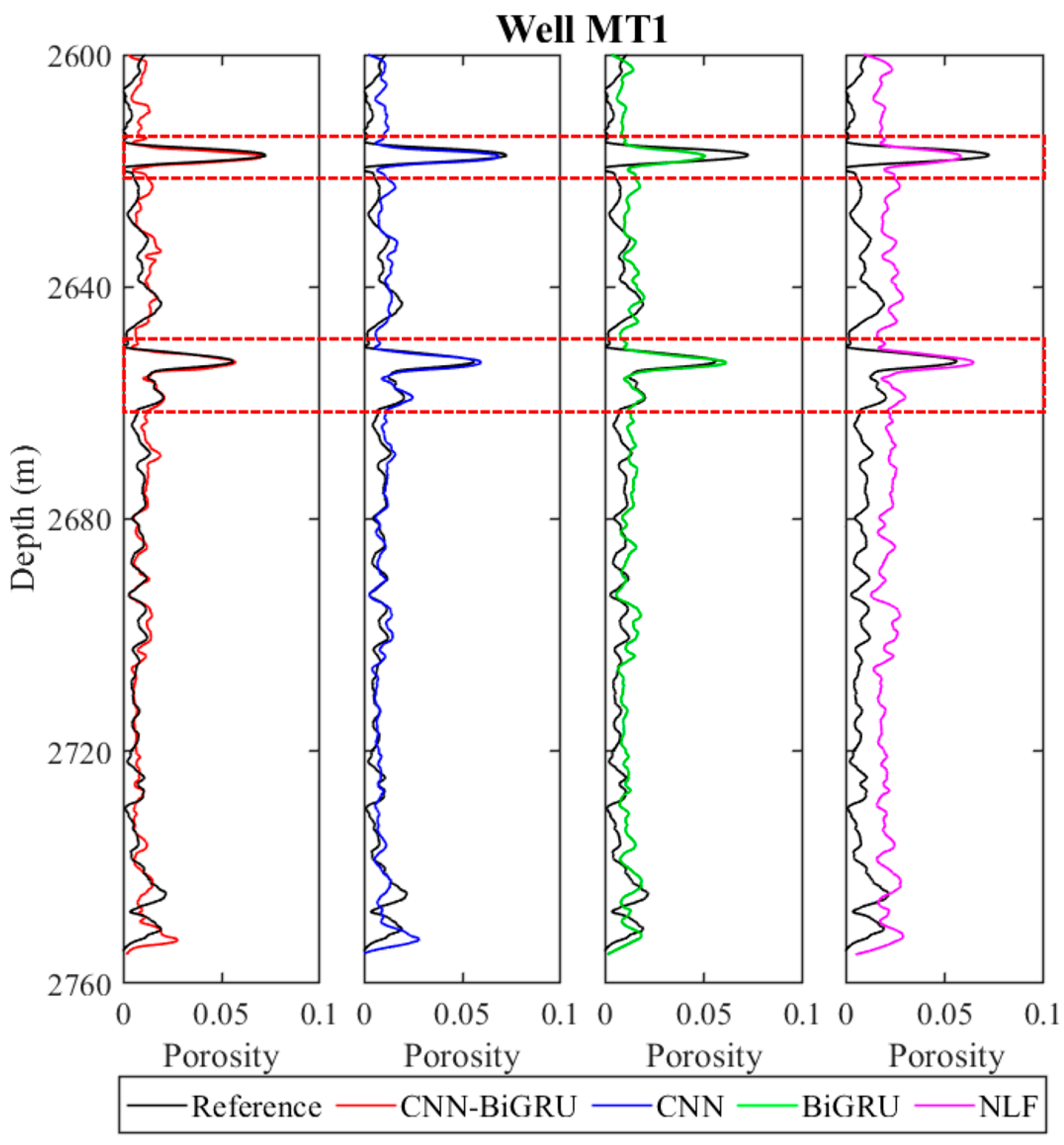
To validate the generalization ability of the proposed CNN–BiGRU, blind well testing is carried out. The evaluation results of the CNN–BiGRU network model are compared with the baseline CNN and BiGRU methods and NLF in well MT 1, as shown in Figure 12. As expected, except for the NLF method, all methods yield reliable results when compared with the porosity log. It is obvious that the trained CNN–BiGRU provides more accurate results, especially at the depths of 2614–2622 m and 2650–2662 m due to its advantages in extracting the feature information of sequence data. The small discrepancy between the estimates and porosity log in the low-porosity intervals is likely due to the heterogeneous pore structures associated with complex geological processes.
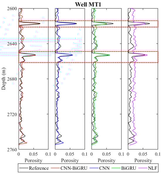
Figure 12.
Porosity evaluation results of well MT 1 using CNN–BiGRU, CNN, BiGRU and NLF methods. All porosity values are smoothed with a 35-point running average. The black curve represents the porosity log taken as the reference; the other red, blue, green and pink curves indicate the porosities estimated based on CNN–BiGRU, CNN, BiGRU, traditional NLF models, respectively. The dashed red boxes mark some areas where the porosity prediction results have been improved by applying the CNN–BiGRU model.
To further assess the precision and efficiency of porosity estimation, the RMSE, PCC and computational time values of the four methods are calculated in Table 1. The statistical results illustrate that the proposed CNN–BiGRU model achieves a lower RMSE of 0.0068 and a higher PCC of 0.983, outperforming those obtained from the CNN, BiGRU and NLF. Due to the complex network architecture, the hybrid model seems to take more computational time than other methods. Overall, the CNN–BiGRU improves the accuracy of porosity evaluation, surpassing the performance of other methods.

Table 1.
Comparison of porosity evaluation errors and calculation efficiency from different models using the RMSE, PCC, and computational time.
5. Application to Seismic Data
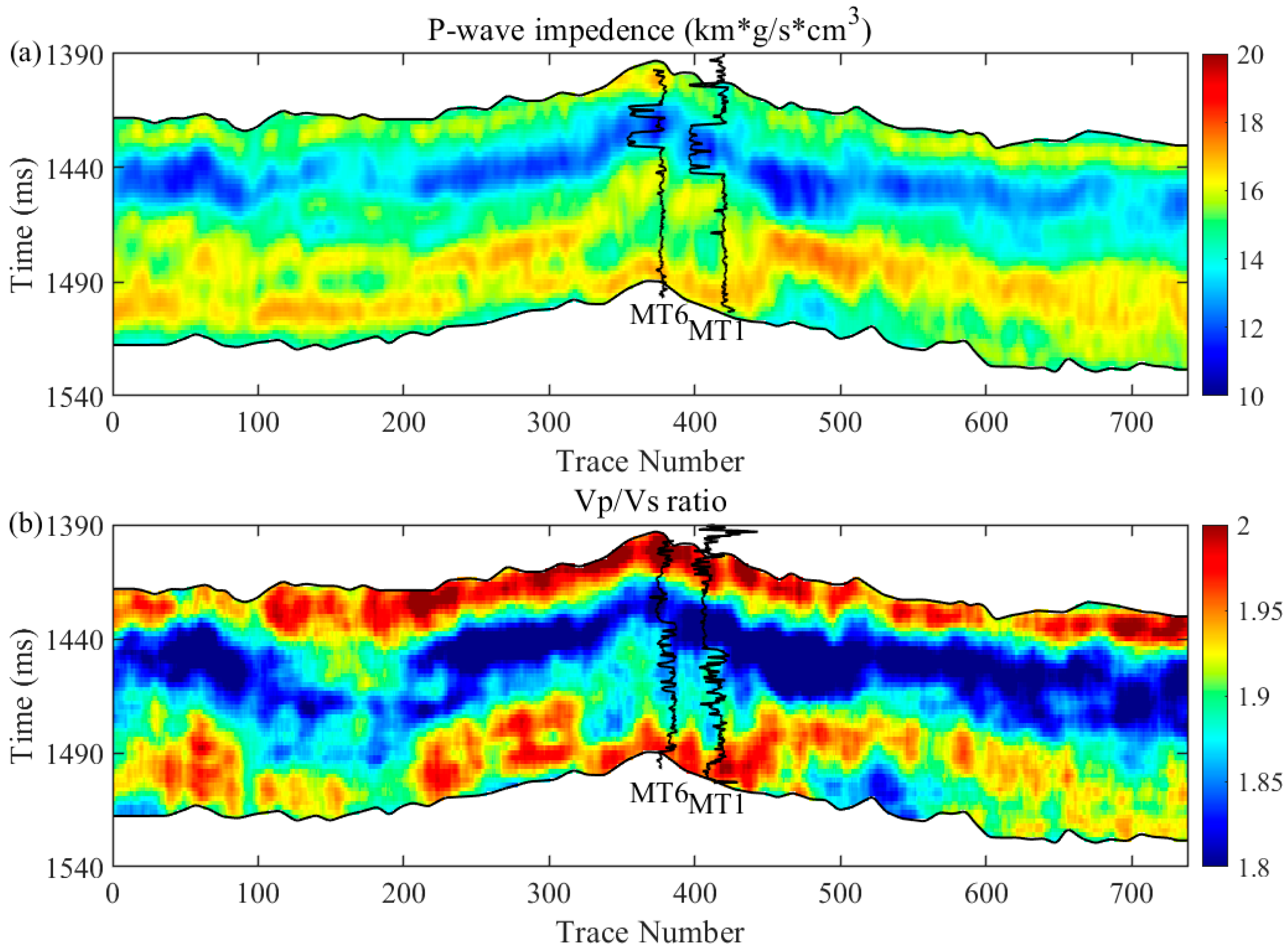
Before predicting reservoir porosity, the P-wave impedance and Vp/Vs ratio are first estimated from pre-stack seismic data using commercial software with strict quality control. Figure 13 shows the inverted cross-well profiles of the P-wave impedance and Vp/Vs ratio. The irregular distribution of elastic properties indicates the strong heterogeneity and poor continuity of the target. Then, the trained CNN–BiGRU is applied to the seismic inversion results to predict porosity.
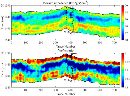
Figure 13.
AVO inversion results of P-wave impedance (a) and Vp/Vs ratio (b) obtained from pre-stack seismic data.
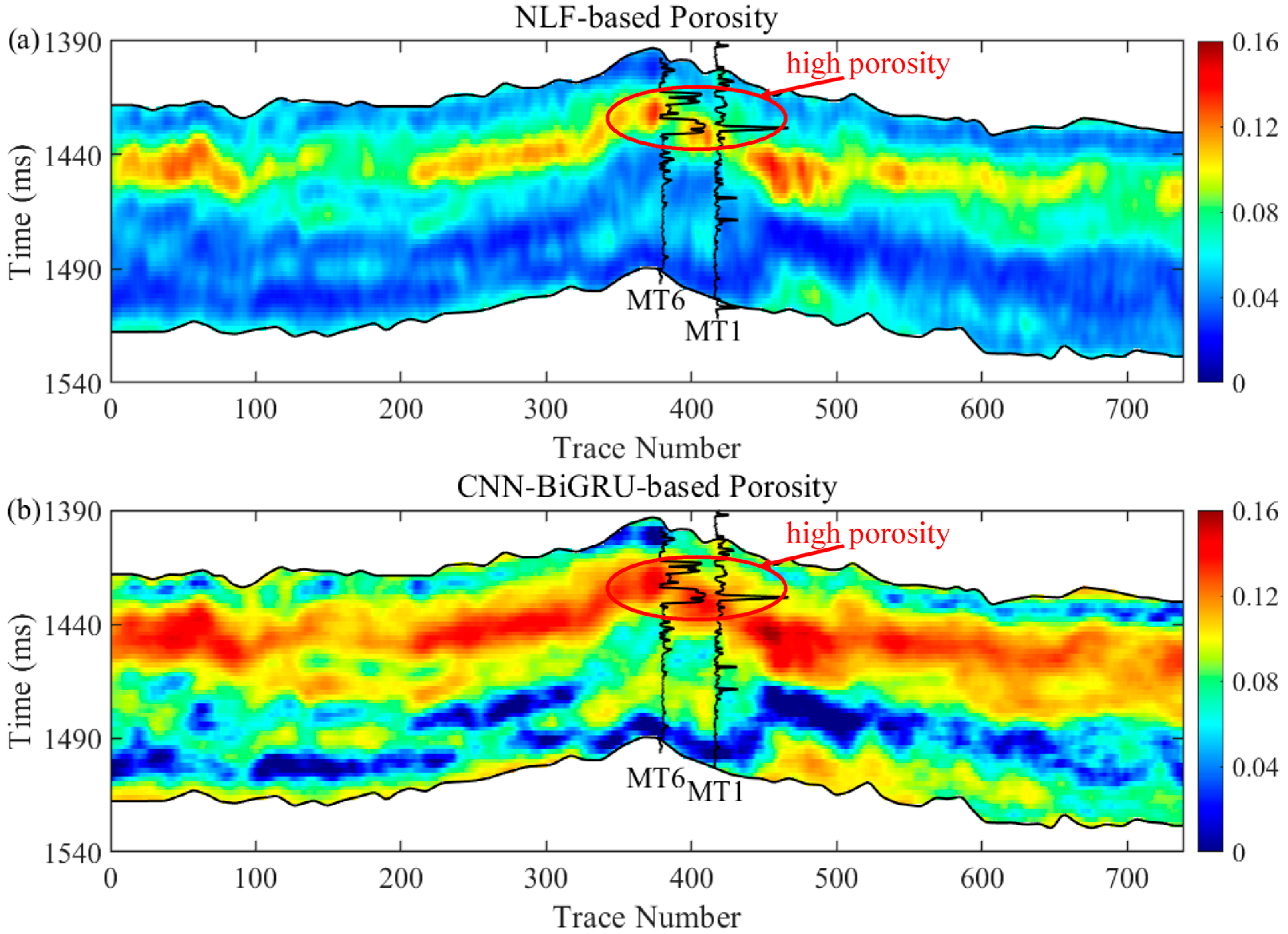
Figure 14 displays the cross-well profiles of porosity estimated from the P-wave impedance and Vp/Vs ratio using the traditional NLF method and the proposed CNN–BiGRU model, respectively. For a comparison of seismic and well-logging data, we superimpose the well-logging porosity of wells MT 6 and MT 1, filtered by high-frequency cutting on the estimated porosity section. It shows that the porosity estimates based on two methods are relatively high around wells MT 6 and MT 1 and match well with the trends in variation in the porosity logs. This is not surprising because both wells are located in the local uplift and faulted zones, favoring the development of micro-cracks or fractures. In addition, the matrix pores, such as intercrystalline, intergranular, and intragranular pores, are well-developed due to the differential compaction, intense dissolution, and penecontemporaneous dolomitization of the target formation. These matrix pores and cracks contribute to increased porosity. Moreover, these findings align with actual production data, which report a daily gas production of 12.2 × 10⁴ m3 from well MT 6 and 35.24 × 10⁴ m3 from well MT 1. In comparison, the CNN–BiGRU-based porosity estimate, ranging from 11.7% to 16%, is more consistent with the porosity logs (11%~21%) around wells MT 6 and MT 1 when compared with the NLF method estimate (8.3%~11.4%) in the 1412~1442 ms section. Therefore, it can be concluded that the CNN–BiGRU model surpasses the NLF algorithm for the seismic estimation of porosity distribution compared to the porosity logs. This comparison demonstrates that the hybrid neural network model effectively captures spatiotemporal characteristics in seismic data and enhances prediction performance.

Figure 14.
The seismic section of inverted porosity by traditional NLF (a) and CNN–BiGRU (b). The upper and low horizon represents the top of Ma 510 and the base of Ma 4. The inverted porosity profile through wells MT 1 and MT 6 are plotted for comparison with the inversion results. The red circle in the plot denotes the high-porosity zone.
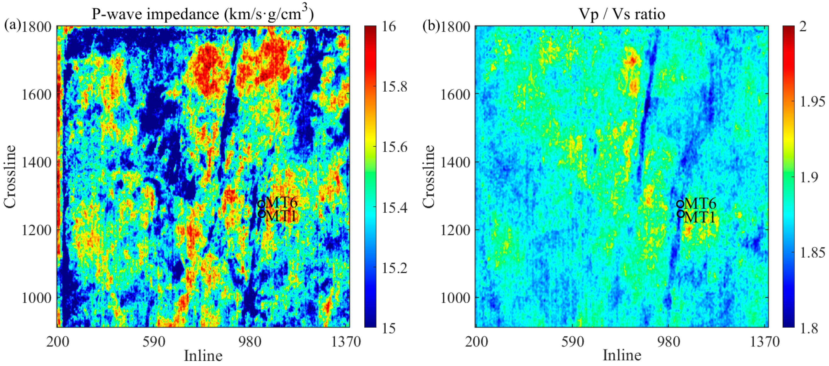
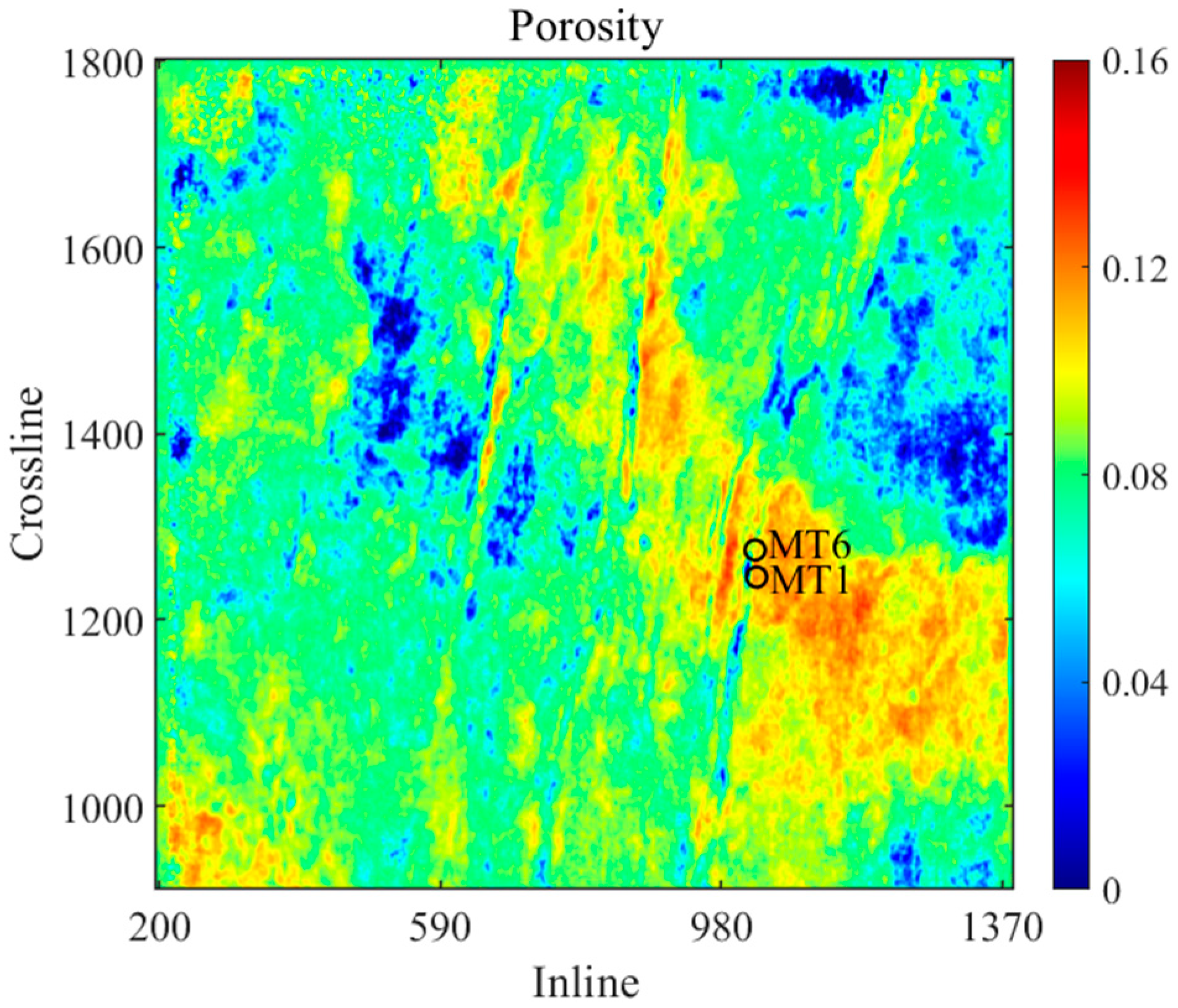
To further predict the spatial distribution of reservoir porosity, the trained CNN–BiGRU model is applied to 3D seismic data. Figure 15 shows the time slice of the P-wave impedance and Vp/Vs ratio data volume obtained via AVO inversion method based on the Aki-Richard equation. These datasets are fed into the trained model to determine the porosity distribution. Two wells are superimposed on the predicted porosity slices for comparison. The porosity values at well sites MT 1 and MT 6 are relatively high (see Figure 16). This is understandable because both wells are located in the Gaojiapu fault zone, where the faults, fractures, and matrix pores are relatively developed. The results show that the CNN–BiGRU model can reliably describe the spatial distribution of porosity in tight carbonate reservoirs.
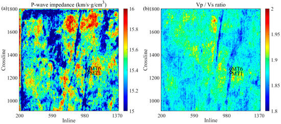
Figure 15.
Time slices of P-wave impedance (a) and Vp/Vs ratio (b) obtained by AVO inversion.

Figure 16.
Porosity time slice predicted using the CNN–BiGRUCNN–BiGRU.
6. Discussion
A hybrid neural network based on CNN and BiGRU is presented to estimate porosity distribution from seismic data. By combining the strengths of CNN and BiGRU in feature extraction and nonlinear representation, the CNN–BiGRU model can capture the spatiotemporal correlations between the input data and target variable (porosity). Although the proposed method provides improved porosity estimates from well logs and seismic data, it still has some limitations. For example, the complex structure of the CNN–BiGRU increases the computational runtime, and thus heavily decreases efficiency in handling large 3D seismic datasets. It also should be noted that the developed CNN–BiGRU model is a supervised learning network, and its prediction performance requires a sufficiently large training dataset. However, this study only used logging data from four wells for training and the data from the remaining fifth well for validation. The insufficient training samples are prone to overfitting and reduce the generalization ability. To this end, physics-based training or unsupervised learning methods are recommended when confronted with a lack of labeled data. In addition, this network establishes a deterministic connection between the input and the output from a given training dataset, and it does not intrinsically measure the prediction uncertainty. Therefore, future work will focus on exploring the uncertainty of porosity estimation to assess the robustness of the model and the reliability of the inversion results.
The experimental results in this work demonstrate that the prediction performance of the CNN–BiGRU model is superior to that of baseline models and traditional methods in terms of prediction accuracy. However, it should be pointed out that only the P-wave impedance and the Vp/Vs ratio are used to invert porosity in these examples. If more seismic data attributes are used as inputs for the CNN–BiGRU model to estimate porosity, the reliability of the inversion results may be further enhanced. Additionally, it is optimal to use the well-log data to train a CNN–BiGRU model and then use seismic data to predict the porosity distribution. Notably, the scale matching between seismic data and logging data may also affect the generalization ability of the trained CNN–BiGRU on seismic data [54]. This issue was addressed by adding dropout and batch normalization layers following the convolutional layers in the network architecture. Apart from porosity estimation, the proposed method is readily extended to pre-stack seismic data for the simultaneous inversion of multiple reservoir properties such as permeability, water saturation, or mineral volume fraction.
7. Conclusions
In this study, a spatiotemporal neural network based on the CNN and BiGRU models is proposed, and a workflow of the CNN–BiGRU-based porosity inversion method for tight carbonate reservoirs is developed. The developed model leverages the advantages of CNN and BiGRU networks by extracting spatial characteristics using the CNNs and learning temporal features using the BiGRU. Once the model is trained, it is easy to obtain the porosity distribution of the target area by feeding the seismic-derived elastic properties to the network. The blind well testing shows that the CNN–BiGRU model has strong generalization ability and prediction accuracy in porosity inversion, outperforming baseline models and the traditional NLF method. The results on real 3D seismic data show the validity of this proposed method. The finding in this study is that the CNN–BiGRU-based method can be used to establish the complex mapping relationship between seismic elastic parameters and the porosity of the complex carbonate reservoir. This approach holds considerable promise for reservoir property prediction and paves a new way to use modern deep-learning methods for the seismic characterization of other complex reservoirs.
Author Contributions
Conceptualization, F.L. (Fei Li) and Z.G.; writing—original draft, F.L. (Fei Li), Z.Y. and Z.G.; methodology, Z.Y. and Z.G.; validation, F.L. (Fei Li), Z.Y., Y.W. and F.L. (Feng Liu); revising, Z.Y., Y.W., F.L. (Feng Liu) and Z.G.; data curation, M.J. and F.L. (Feng Liu); supervision, F.L. (Fei Li) and Z.G. All authors have read and agreed to the published version of the manuscript.
Funding
This work is funded by the National Engineering Laboratory for Exploration and Development of Low-permeability Oil and Gas Fields (KFKT2023-20).
Data Availability Statement
The data that support the findings of this study are available from the Zhiyi Yu. Corporation (CNPC), for sample preparation, and are grateful for their support.
Conflicts of Interest
Authors Fei Li, Yonggang Wang, Meixin Ju and Feng Liu were employed by the company Exploration and Development Research Institute of Changqing Oilfield Branch Company Ltd. The authors declare that they have no known competing financial interests or personal relationships that could have appeared to influence the work reported in this paper.
Nomenclature
| Abbreviation | Definition |
| AVO | Amplitude variation with offset |
| IP | P-wave impedance |
| Porosity | |
| CNN | Convolutional neural network |
| RNN | Recurrent neural network |
| LSTM | Long short-term memory neural network |
| GRU | Gated recurrent unit |
| BiGRU | Bidirectional gated recurrent unit |
| CNN–BiGRU | A hybrid network incorporating CNN and BiGRU |
| NLF | Nonlinear fitting |
| RMSE | Root mean square error |
| PCC | Pearson correlation coefficient |
References
- Zou, C.; Zhao, L.; Xu, M.; Chen, Y.; Geng, J. Porosity prediction with uncertainty quantification from multiple seismic attributes using random forest. J. Geophys. Res. Solid Earth 2021, 126, e2021JB021826. [Google Scholar] [CrossRef]
- Liu, S.; Liu, Z.; Zhang, Z. Numerical study on hydraulic fracture-cavity interaction in fractured-vuggy carbonate reservoir. J. Pet. Sci. Eng. 2022, 213, 110426. [Google Scholar] [CrossRef]
- Liu, J.; Zhao, L.; Xu, M.; Zhao, X.; You, Y.; Geng, J. Porosity prediction from prestack seismic data via deep learning: Incorporating a low-frequency porosity model. J. Geophys. Eng. 2023, 20, 1016–1029. [Google Scholar] [CrossRef]
- Xu, S.; Payne, M.A. Modeling elastic properties in carbonate rocks. Lead. Edge 2009, 28, 66–74. [Google Scholar] [CrossRef]
- Zhao, L.; Nasser, M.; Han, D.H. Quantitative geophysical pore-type characterization and its geological implication in carbonate reservoirs. Geophys. Prospect. 2013, 61, 827–841. [Google Scholar] [CrossRef]
- Fournier, F.; Pellerin, M.; Villeneuve, Q.; Teillet, T.; Hong, F.; Poli, E.; Borgomano, J.; Léonide, P.; Hairabian, A. The equivalent pore aspect ratio as a tool for pore type prediction in carbonate reservoirs. AAPG Bull. 2018, 102, 1343–1377. [Google Scholar] [CrossRef]
- Guo, Q.; Ba, J.; Fu, L.Y.; Luo, C. Joint seismic and petrophysical nonlinear inversion with Gaussian mixture-based adaptive regularization. Geophysics 2021, 86, R895–R911. [Google Scholar] [CrossRef]
- Du, M.; Pan, H.; Wei, C.; Li, H.; Cai, S.; Huang, C.; Gui, Z. Simultaneous quantification of triple pore types in carbonate reservoirs using well logs and seismic data. Geophysics 2024, 89, M211–M226. [Google Scholar] [CrossRef]
- Pan, H.J.; Wei, C.; Yan, X.F.; Li, X.M.; Yang, Z.F.; Gui, Z.X.; Liu, S.-X. 3D rock physics template-based probabilistic estimation of tight sandstone reservoir properties. Pet. Sci. 2024, 21, 3090–3101. [Google Scholar] [CrossRef]
- Feng, R.; Mejer Hansen, T.; Grana, D.; Balling, N. An unsupervised deep-learning method for porosity estimation based on poststack seismic data. Geophysics 2020, 85, M97–M105. [Google Scholar] [CrossRef]
- Liu, X.; Zhou, H.; Guo, K.; Li, C.; Zu, S.; Wu, L. Quantitative characterization of shale gas reservoir properties based on BiLSTM with attention mechanism. Geosci. Front. 2023, 14, 101567. [Google Scholar] [CrossRef]
- Alfarraj, M.; AlRegib, G. Semisupervised sequence modeling for elastic impedance inversion. Interpretation 2019, 7, SE237–SE249. [Google Scholar] [CrossRef]
- Wu, X.; Yan, S.; Bi, Z.; Zhang, S.; Si, H. Deep learning for multidimensional seismic impedance inversion. Geophysics 2021, 86, R735–R745. [Google Scholar] [CrossRef]
- Wang, Y.Q.; Wang, Q.; Lu, W.K.; Ge, Q.; Yan, X.F. Seismic impedance inversion based on cycle-consistent generative adversarial network. Pet. Sci. 2022, 19, 147–161. [Google Scholar] [CrossRef]
- Biswas, R.; Sen, M.K.; Das, V.; Mukerji, T. Prestack and poststack inversion using a physics-guided convolutional neural network. Interpretation 2019, 7, SE161–SE174. [Google Scholar] [CrossRef]
- Cao, D.; Su, Y.; Cui, R. Multi-parameter pre-stack seismic inversion based on deep learning with sparse reflection coefficient constraints. J. Pet. Sci. Eng. 2022, 209, 109836. [Google Scholar] [CrossRef]
- Singh, P.K.; Shankar, U. Estimation of reservoir properties using pre-stack seismic inversion and neural network in mature oil field, Upper Assam basin, India. J. Appl. Geophys. 2024, 230, 105523. [Google Scholar] [CrossRef]
- Rezaee, M.R.; Ilkhchi, A.K.; Barabadi, A. Prediction of shear wave velocity from petrophysical data utilizing intelligent systems: An example from a sandstone reservoir of Carnarvon Basin, Australia. J. Pet. Sci. Eng. 2007, 55, 201–212. [Google Scholar] [CrossRef]
- Wang, J.; Cao, J.; Zhao, S.; Qi, Q. S-wave velocity inversion and prediction using a deep hybrid neural network. Sci. China Earth Sci. 2022, 65, 724–741. [Google Scholar] [CrossRef]
- Hayashi, K.; Suzuki, T.; Inazaki, T.; Konishi, C.; Suzuki, H.; Matsuyama, H. Estimating S-wave velocity profiles from horizontal-to-vertical spectral ratios based on deep learning. Soils Found. 2024, 64, 101525. [Google Scholar] [CrossRef]
- Liu, Y.; Gao, C.; Zhao, B. Shear-wave velocity prediction based on the CNN-BiGRU integrated network with spatiotemporal attention mechanism. Processes 2024, 12, 1367. [Google Scholar] [CrossRef]
- Alqahtani, N.; Armstrong, R.T.; Mostaghimi, P. Deep learning convolutional neural networks to predict porous media properties. In Proceedings of the SPE Asia Pacific Oil and Gas Conference and Exhibition, Brisbane, Australia, 23–25 October 2018; SPE: Milwaukee, WI, USA, 2018; p. D012S032R010. [Google Scholar]
- Graczyk, K.M.; Matyka, M. Predicting porosity, permeability, and tortuosity of porous media from images by deep learning. Sci. Rep. 2020, 10, 21488. [Google Scholar] [CrossRef] [PubMed]
- Jo, H.; Cho, Y.; Pyrcz, M.; Tang, H.; Fu, P. Machine-learning-based porosity estimation from multifrequency poststack seismic data. Geophysics 2022, 87, M217–M233. [Google Scholar] [CrossRef]
- Wang, Y.Y.; Niu, L.P.; Zhao, L.X.; Wang, B.F.; He, Z.L.; Zhang, H.; Chen, D.; Geng, J.H. Gaussian mixture model deep neural network and its application in porosity prediction of deep carbonate reservoir. Geophysics 2022, 87, M59–M72. [Google Scholar] [CrossRef]
- Zhang, H.; Wu, W. Shale content prediction of well logs based on CNN-BiGRU-VAE neural network. J. Earth Syst. Sci. 2023, 132, 139. [Google Scholar] [CrossRef]
- Aljubran, M.; Ramasamy, J.; Albassam, M.; Magana-Mora, A. Deep learning and time-series analysis for the early detection of lost circulation incidents during drilling operations. IEEE Access 2021, 9, 76833–76846. [Google Scholar] [CrossRef]
- Onwuchekwa, C. Application of machine learning ideas to reservoir fluid properties estimation. In Proceedings of the SPE Nigeria Annual International Conference and Exhibition, Lagos, Nigeria, 6–8 August 2018; SPE: Milwaukee, WI, USA, 2018; p. SPE-193461. [Google Scholar]
- Zhang, G.; Wang, Z.; Chen, Y. Deep learning for seismic lithology prediction. Geophys. J. Int. 2018, 215, 1368–1387. [Google Scholar] [CrossRef]
- Zhang, J.; Li, J.; Chen, X.; Li, Y. Seismic lithology/fluid prediction via a hybrid ISD-CNN. IEEE Geosci. Remote Sens. Lett. 2020, 18, 13–17. [Google Scholar] [CrossRef]
- Hussain, M.; Liu, S.; Hussain, W.; Liu, Q.; Hussain, H.; Ashraf, U. Application of Deep Learning for Reservoir Porosity Prediction and Self Organizing Map for Lithofacies Prediction. J. Appl. Geophys. 2024, 230, 105502. [Google Scholar] [CrossRef]
- Mandelli, S.; Lipari, V.; Bestagini, P.; Tubaro, S. Interpolation and denoising of seismic data using convolutional neural networks. arXiv 2019, arXiv:1901.07927. [Google Scholar]
- Richardson, A.; Feller, C. Seismic data denoising and deblending using deep learning. arXiv 2019, arXiv:1907.01497. [Google Scholar]
- Yu, S.; Ma, J.; Wang, W. Deep learning for denoising. Geophysics 2019, 84, V333–V350. [Google Scholar] [CrossRef]
- Das, V.; Pollack, A.; Wollner, U.; Mukerji, T. Convolutional neural network for seismic impedance inversion. Geophysics 2019, 84, R869–R880. [Google Scholar] [CrossRef]
- Yang, N.; Li, G.; Zhao, P.; Zhang, J.; Zhao, D. Porosity prediction from pre-stack seismic data via a data-driven approach. J. Appl. Geophys. 2023, 211, 104947. [Google Scholar] [CrossRef]
- Hourcade, C.; Bonnin, M.; Beucler, É. New CNN-based tool to discriminate anthropogenic from natural low magnitude seismic events. Geophys. J. Int. 2023, 232, 2119–2132. [Google Scholar] [CrossRef]
- Wang, J.; Cao, J.; Fu, J.; Xu, H. Missing well logs prediction using deep learning integrated neural network with the self-attention mechanism. Energy 2022, 261, 125270. [Google Scholar] [CrossRef]
- Di, H.; Abubakar, A. A CNN-accelerated workflow for stochastic seismic property estimation. Geophysics 2024, 90, IM35–IM45. [Google Scholar] [CrossRef]
- Shan, L.; Liu, Y.; Tang, M.; Yang, M.; Bai, X. CNN-BiLSTM hybrid neural networks with attention mechanism for well log prediction. J. Pet. Sci. Eng. 2021, 205, 108838. [Google Scholar] [CrossRef]
- Zhang, J.; Liu, Z.; Zhang, G.; Yan, B.; Ni, X.; Xie, T. Simultaneous prediction of multiple physical parameters using gated recurrent neural network: Porosity, water saturation, shale content. Front. Earth Sci. 2022, 10, 984589. [Google Scholar] [CrossRef]
- Wang, J.; Cao, J. A lithology identification approach using well logs data and convolutional long short-term memory networks. IEEE Geosci. Remote Sens. Lett. 2023, 20, 7506405. [Google Scholar] [CrossRef]
- Soares, L.D.; Franco EM, C. BiGRU-CNN neural network applied to short-term electric load forecasting. Production 2021, 32, e20210087. [Google Scholar] [CrossRef]
- Li, X.; Zhou, S.; Wang, F. A CNN-BiGRU sea level height prediction model combined with bayesian optimization algorithm. Ocean. Eng. 2025, 315, 119849. [Google Scholar] [CrossRef]
- Wang, T.; Fu, L.; Zhou, Y.; Gao, S. Service price forecasting of urban charging infrastructure by using deep stacked CNN-BiGRU network. Eng. Appl. Artif. Intell. 2022, 116, 105445. [Google Scholar] [CrossRef]
- Wang, J.; Cao, J.; Yuan, S. Deep learning reservoir porosity prediction method based on a spatiotemporal convolution bi-directional long short-term memory neural network model. Geomech. Energy Environ. 2022, 32, 100282. [Google Scholar] [CrossRef]
- Jung, W.; Jung, D.; Kim, B.; Lee, S.; Rhee, W.; Ahn, J.H. Restructuring batch normalization to accelerate CNN training. Proc. Mach. Learn. Syst. 2019, 1, 14–26. [Google Scholar]
- Hochreiter, S. Long Short-term Memory. Neural Comput. 1997, 9, 1735–1780. [Google Scholar] [CrossRef] [PubMed]
- Chung, J.; Gulcehre, C.; Cho, K.; Bengio, Y. Empirical evaluation of gated recurrent neural networks on sequence modeling. arXiv 2014, arXiv:1412.3555. [Google Scholar]
- Cho, K.; Van Merriënboer, B.; Gulcehre, C.; Bahdanau, D.; Bougares, F.; Schwenk, H.; Bengio, Y. Learning phrase representations using RNN encoder-decoder for statistical machine translation. arXiv 2014, arXiv:1406.1078. [Google Scholar]
- Busch, P.; Lahti, P.; Werner, R.F. Colloquium: Quantum root-mean-square error and measurement uncertainty relations. Rev. Mod. Phys. 2014, 86, 1261–1281. [Google Scholar] [CrossRef]
- Cohen, I.; Huang, Y.; Chen, J.; Benesty, J.; Benesty, J.; Chen, J.; Huang, Y.; Cohen, I. Pearson correlation coefficient. In Noise Reduction in Speech Processing; Springer Science and Business Media: New York, NY, USA, 2009; pp. 1–4. [Google Scholar]
- Chen, X.; Dong, J.; Wang, B.; Li, W.; Ma, J. A Novel Method to Predict S-Wave Velocity of Carbonate Based on Variable Matrix and Equivalent Porous Medium Model. Geofluids 2024, 2024, 9285032. [Google Scholar] [CrossRef]
- Srivastava, N.; Hinton, G.; Krizhevsky, A.; Sutskever, I.; Salakhutdinov, R. Dropout: A simple way to prevent neural networks from overfitting. J. Mach. Learn. Res. 2014, 15, 1929–1958. [Google Scholar]
- Kingma, D.P. Adam: A method for stochastic optimization. arXiv 2014, arXiv:1412.6980. [Google Scholar]

Disclaimer/Publisher’s Note: The statements, opinions and data contained in all publications are solely those of the individual author(s) and contributor(s) and not of MDPI and/or the editor(s). MDPI and/or the editor(s) disclaim responsibility for any injury to people or property resulting from any ideas, methods, instructions or products referred to in the content. |
© 2025 by the authors. Licensee MDPI, Basel, Switzerland. This article is an open access article distributed under the terms and conditions of the Creative Commons Attribution (CC BY) license (https://creativecommons.org/licenses/by/4.0/).