Abstract
The location of faults in distribution networks represents a crucial line of defence, ensuring the safe and reliable operation of these networks. This paper puts forth a methodology for the location of short-circuit faults between phases within the context of a distribution network information physics system. Firstly, a distribution network topology identification model is constructed, and a switching function based on the characteristics of an interphase short-circuit fault current is constructed to form a physical layer interphase short-circuit preconceived fault set. Subsequently, methodologies for processing information perturbations, including distortion, delay, and failure, are proposed. Fault current information is then extracted to form an information layer fault current array. Ultimately, a similarity function is constructed to correlate the fault characteristics of the physical and information layers. This is achieved through the utilization of the variational bee colony algorithm, which is employed to address the aforementioned issue. The efficacy and suitability of the proposed methodology are assessed in the context of single-point and multi-point faults, dynamic topology alterations, and information perturbations in distribution networks. To this end, a real-world project in Hebei and the IEEE system are employed as illustrative examples. The methodology proposed in this paper can facilitate the rapid and precise location of phase-to-phase short-circuits in physical information systems of distribution networks, thereby enhancing the reliability of power supply in new intelligent distribution networks.
1. Introduction
As more and more monitoring and communication devices are applied in distribution networks [1], distribution networks are gradually evolving into a distribution cyber physical system (DCPS) with a high degree of information–physical integration, and DCPSs are facing more complex operation scenarios, which bring new challenges to the traditional fault location in distribution networks [2]. At the information level, there are phenomena such as disturbances or delays in data collection and transmission in the power system communication network which can affect the normal dissemination of fault information [3]. At the physical level, the flexibility of distribution networks is increasing, and the applicability of fault location techniques for fixed topologies is limited [4]; there is an urgent need to develop phase-to-phase short-circuit fault location techniques applicable to the information–physical system of distribution networks.
Distribution network fault location methods can be divided into two categories: ranging and segmentation. The ranging method is used to determine the location of the fault distance measurement point by calculating the electrical distance between the measurement point and the fault point, and there are two main forms of calculation. One is to rely on the transmission time of the fault signal or electromagnetic distribution characteristics to calculate the location of the measurement point to the fault point [5]. This is exemplified in a study [6] which proposed a fault ranging method based on the travelling wave modal decomposition of the distribution network, calculating the distance between the first travelling wave of the voltage travelling wave and the refracted wave head to achieve the fault location. Another study [7] extracted the electromagnetic field characteristics generated by measuring the transient amount of fault current, transformed the ranging problem into the field strength distribution problem of the electromagnetic field, and realized the fault point location within a short time window. Another ranging method is to analyze and calculate the line impedance between two points to calculate the distance to the fault point, exemplified in a study [8] which used an impedance method based on zero-sequence component distribution network fault location technology according to the zero-sequence voltage at both ends of the line, the bus side zero sequence current, and the line zero sequence parameter, to establish the impedance ranging equations of each section when a single-phase ground fault occurs and solve the distance to the fault point. Another study [9] deduced the relationship between zero-sequence voltage, current, and line impedance at the first and last ends of the faulted section according to the principle of minimum zero-sequence voltage at the fault point, and solved the ranging equations by using the joint search of the advance and retreat–golden division method. The two types of ranging methods are faster in calculation, but their positioning accuracy and precision depend on the accuracy and precision of the measurement signal. Compared to traditional distribution networks, the probability of disturbance during the transmission of measurement signals in DCPS increases [10], which affects the positioning results, so the applicability of ranging methods in DCPS is limited.
The fixed-segment method analyzes electrical information such as voltage, current and phase in the feeder through the main station of the distribution management system and determines the feeder segments with abnormal status to obtain the fault location. There are two main types of calculation methods in the fixed segment method, in which the matrix algorithm outputs feeder segment state information by constructing the distribution network structure description and outputs fault segments according to the state criterion. One study [11] established fault current information and the fault line segment correlation matrix according to the topology of the distribution network, taking the current as the line state judgement index to identify feeder segments with abnormal states to achieve fault locations. Another study [12] established the correlation matrix between feeder segments and nodes based on the actual structure of the distribution network, taking the node voltage as the fault criterion, and achieving fault location by identifying feeder segments with abnormal node voltages at both ends. In the matrix algorithm, the accuracy of the collected and transmitted information affects the accuracy of the elements in the matrix as well as the state of the feeder segment, which in turn affects the fault location. Another method of segment fixing is the fault feature matching method. For example, one study [13] analyzed the fault current information samples collected under different feeder segment fault conditions to construct the operating history fault set the next morning, and based on artificial neural network, self-learning categorized the real-time collected fault current information to achieve the fault location. Another study [14,15] used a method based on the current calculation to analyze the current changes in the feeder section after the fault to construct the expected fault set, and, respectively, used the improved whale algorithm and the improved vulture search algorithm to match the actual fault current characteristics with the individuals in the expected fault set for optimization to find the most compatible fault situation to achieve the fault location. In the actual system, the distribution network fault data samples are small, leading to the difficulty of constructing the historical fault set, and as the current distribution network scale increases, topology flexibility increases; the current research related to fault state matching method is insufficient to consider the flexibility characteristics of the distribution network [16].
In order to adapt to the current situation of dynamic topology change and the increased probability of information perturbation during the operation of the new smart distribution network, this paper comprises research on the phase-to-phase short-circuit fault location method of the distribution network information physics system. By identifying the distribution network topology online, constructing the physical layer’s pre-conceived fault set, and forming the information layer fault current array based on the analysis of the impact of information perturbation on the fault current information, the variational bee colony algorithm is used to solve the similarity of the fault characteristics of the physical layer and the information layer, so as to achieve the fast and accurate positioning of short-circuit faults between the phases of the distribution network.
2. Physical Layer Predictive Fault Set Construction
Among these short-circuit faults in power systems, two-phase short-circuit and single-phase-to-ground short-circuit are the most common and worthy of in-depth study in the context of interphase short-circuits and phase-to-ground short-circuits [17].
The two-phase short-circuit occurs between two phase conductors. When it happens, the current in the fault phases surges, which can disrupt the normal operation of electrical equipment connected to these phases. It often leads to local power outages and may even cause a chain reaction, expanding the scope of the fault.
The single-phase-to-ground short-circuit, on the other hand, is prevalent in power systems, especially in neutral ungrounded systems. It can cause abnormal ground currents, which not only interfere with the normal operation of the power grid but also pose potential threats to equipment and personnel safety.
Given the high frequency and potential hazards of these two types of short-circuit faults, our paper focuses on developing advanced fault location and protection strategies. We aim to improve the reliability and safety of power systems by accurately identifying the location of two-phase short-circuit and single-phase-to-ground short-circuit faults. Through in-depth research on fault characteristics, we propose innovative methods to quickly detect and isolate these faults, reducing the impact on power supply and minimizing the risk of equipment damage and safety accidents.
Firstly, the optimal identification model of distribution network topology is constructed. Secondly, on the basis of determining the topology, the characteristics of interphase short-circuit fault currents are analyzed, and then the switching function is constructed based on the current changes in the feeder segments before and after the faults. Finally, based on the switching function, the expected fault current array of the system is calculated at the time of faults at each node to obtain the expected fault set of the physical system.
2.1. Distribution Network Topology Identification
In the actual system, the topology of the distribution network will be changed due to the increase or decrease in feeder segments or distributed power sources, and the construction of the expected fault set is based on the topology of the distribution network, so it is necessary to first identify the topology of the distribution network. In this paper, we adopt the method of identifying the topology of the distribution network based on the current distribution [18,19], with the objective of minimizing the absolute error between the actual collected currents and the expected topology currents, constructing an optimization model for topology identification, and expressing the objective function of the topology identification problem as:
where is the branch current phase between the node and the node , is the order-weighted adjacency matrix, which is determined by the number of nodes in the network and the original topology; is the node state monitoring matrix, which is determined by the configuration position of the FTU (feeder terminal unit), and the corresponding element of the position is one at the time of configuration; and is the node injection current phase.
The constraints of the topology identification model are shown in Equations (2)–(5):
Equation (2) is Kirchhoff’s current law constraint, the current phase injected into the node is equal to the sum of the branch current phase connected to the node; Equation (3) is Kirchhoff’s voltage law constraint, is the node voltage phase; indicates the switching state of the branch between the nodes , the branch is closed to take 1, and vice versa to take 0; Equation (4) is the injected power constraint, is the node-injected power; Equation (5) is the connection constraint of the node, and is the number of end nodes.
The Cplex solver can be used to obtain the branch connection state between nodes with the highest matching degree with the current trend distribution.
2.2. Characterization of Short-Circuit Fault Currents Between Phases
A typical distribution network structure is shown in Figure 1.

Figure 1.
Schematic diagram of phase-to-phase short-circuit faults in distribution networks.
The system power supply to the fault point is called the upstream section, and the fault point to the end of the line or distributed power supply becomes the downstream section, when a two-phase short-circuit fault occurs between phases B and C, set , , , respectively, as the three-phase current of phase A, B, and C in the fault line upstream section, , , respectively, as the two-phase fault current of phase B and C at the fault point, , , , respectively, for the three-phase fault voltage of phase A, B and C at the fault point. is the equivalent impedance from the fault point to the end of the line. is the A-phase positive sequence current of the line, is the pre-fault line voltage at the fault point, is the sum of equivalent positive sequence impedance of the line. Using the symmetrical component method of analysis, the three-phase currents in the upstream section can be obtained as [20]:
Similarly, the fault current in each phase of the downstream section line is:
The coupled Equations (6) and (7) yields:
where , is the pre-fault B, C two-phase voltage at fault point F. Analyzing Equations (6)–(8), it can be seen that, when interphase short-circuit fault occurs, the direction of the fault current in the downstream section of the fault point is opposite to the pre-fault. The direction of the fault current in the upstream section is the same as before the fault, so the line current characteristic information before and after the fault can be utilized to construct the predicted fault set.
2.3. Characterization of Short-Circuit Fault Currents Between Phase and Ground
Assuming a single-phase-to-ground fault occurs on phase C of the transmission line, and neglecting the voltage drop caused by the capacitive current in the line, the post-fault voltage of phase C drops to zero, while the voltages of phases A and B increase to times their pre-fault values.
where , , and represent the phase voltages of the three-phase power supply. Under this condition, the zero-sequence voltage at the neutral point equals the system’s phase voltage during normal operation.
The ground capacitive currents of each phase in the healthy line can be expressed as:
where represents the ground capacitance of the healthy line. Therefore, the zero-sequence current flowing through the sending end of the healthy line can be expressed as:
The ground capacitive currents of each phase in the faulted line can be expressed as:
where is defined as the ground capacitance of the faulted line, and represents the sum of the ground capacitances of all branches. Therefore, the zero-sequence current flowing through the sending end of the faulted line can be expressed as:
The integration of distributed generation (DG) will alter the distribution of zero-sequence currents after a fault compared to radial network topologies. Therefore, it is necessary to analyze the impact of DG integration on post-fault zero-sequence currents. When the faulted line is not integrated with DG, the connection of DG to other lines does not significantly affect the zero-sequence current in the faulted line and consequently has negligible influence on fault location accuracy.
When a single-phase-to-ground fault occurs upstream of the DG, the line simultaneously exhibits capacitive currents flowing from the fault point to both the busbar and the DG, with the total current at the fault point equaling the sum of non-fault-phase capacitive currents across the entire system. In non-faulted lines, the zero-sequence current remains the ground capacitive current of non-fault phases, flowing from the busbar to the line. However, the faulted line integrated with DG exhibits distinct zero-sequence current distribution compared to radial networks, manifesting as capacitive currents flowing from the DG to the busbar on its non-fault phases. Downstream of the fault point, the capacitive current on the faulted phase exceeds the sum of non-fault-phase currents due to current diversion through ground capacitance between the fault point and DG on non-fault phases combined with contributions from capacitive currents in the DG downstream section, ultimately driving a zero-sequence current from the fault point toward the line terminal.
Upstream of the fault point, the direction of capacitive currents on the non-fault phases of the faulted line cannot be definitively determined. Even if capacitive currents flow from the busbar toward the fault point, the capacitive current on the faulted phase exceeds the sum of non-fault phase currents due to current diversion through the ground capacitance between the busbar and fault point combined with contributions from non-faulted line capacitive currents, resulting in a zero-sequence current flowing from the fault point to the busbar.
When a single-phase-to-ground fault occurs downstream of the DG, the faulted line exhibits capacitive current flowing exclusively from the fault point to the DG, with the total fault current equaling the sum of capacitive currents from all non-fault phases across the system. In non-faulted lines, the zero-sequence current remains the ground capacitive current of non-fault phases, flowing from the busbar to the lines. Within the faulted line, downstream of the fault point, the zero-sequence current corresponds to the capacitive currents on non-fault phases flowing toward the line terminal, while upstream of the fault point, the capacitive current on the faulted phase exceeds the sum of non-fault phase currents due to current diversion through the ground capacitance between the fault point and DG combined with contributions from non-faulted lines’ capacitive currents, resulting in a zero-sequence current flowing from the fault point to the busbar.
Based on the above conclusions, even in systems integrated with DG, the zero-sequence current upstream of the fault point flows from the fault point to the busbar, while the zero-sequence current downstream of the fault point flows from the fault point to the line terminal during a single-phase-to-ground fault. This directional characteristic of fault currents resembles that of phase-to-phase short-circuit faults, and thus the same methodology can be applied for fault localization.
2.4. Switching Function Construction
The fault current processing value is taken as 0 to indicate that there is no fault current, 1 to indicate that the fault current is in the same direction as the positive direction, and −1 to indicate that the fault current is in the opposite direction of the positive direction, which characterizes the fault current information of each feeder segment of the fault, and defines the switching function :
In the formula, , respectively for the upper half of the region, the lower half of the power supply access, access to take 1, no access to take 0; denotes the logical or operation, , denote OR operations that represent the currents in all feeder segments upstream and downstream of switch , represents the OR operation of switch to the upper half of the power switch state, represents the OR operation of switch to the lower half of the power switch state. This function can be used to reflect the distribution network line operating state and the direct relationship between the various switching nodes.
Based on the switching function, the expected fault current array of the system at the time of failure of each node can be calculated to obtain the expected fault set of the physical system, and when the fault information uploaded from the information layer is received, the fault information is co-matched with the expected fault set to find out the most matching fault situation, so as to realize the fast and accurate location.
3. Information Layer Fault Current Information Feature Modelling
Fault current information feature modelling requires discretization of the current information collected and uploaded by the FTU and processing of the perturbation information to generate the actual fault current array.
3.1. Fault Current Array Construction
In order to describe whether there is a fault current flowing in the physical layer node and the direction of the current, the FTU calculates the raw signals to obtain the current collection value by using Fourier’s algorithm [21]:
where and are the real and imaginary parts of the current information collected by the FTU, is the number of collection points in one cycle, is the number of collection times, and is the collection value of the current.
Find the current magnitude and phase angle from , . The magnitude is I:
The phase angle α of the current is calculated to be:
The FTU current acquisition values are discretized according to Equation (14):
where is the processing value of the FTU fault current collection value, indicates the maximum rated current of the line, and is the fault current discrimination coefficient, which is generally between 1.2 and 1.4. In this paper, it is stipulated that the direction of overcurrent flowing from the system power supply to the load or distributed power supply is positive. A fault current processing value of 0 means no fault current, 1 means that the fault current is in the same direction as the positive direction, and −1 means that the fault current is in the opposite direction to the positive direction, which converts the FTU acquisition value into binary data describing the presence or absence of overcurrent and the direction of overcurrent.
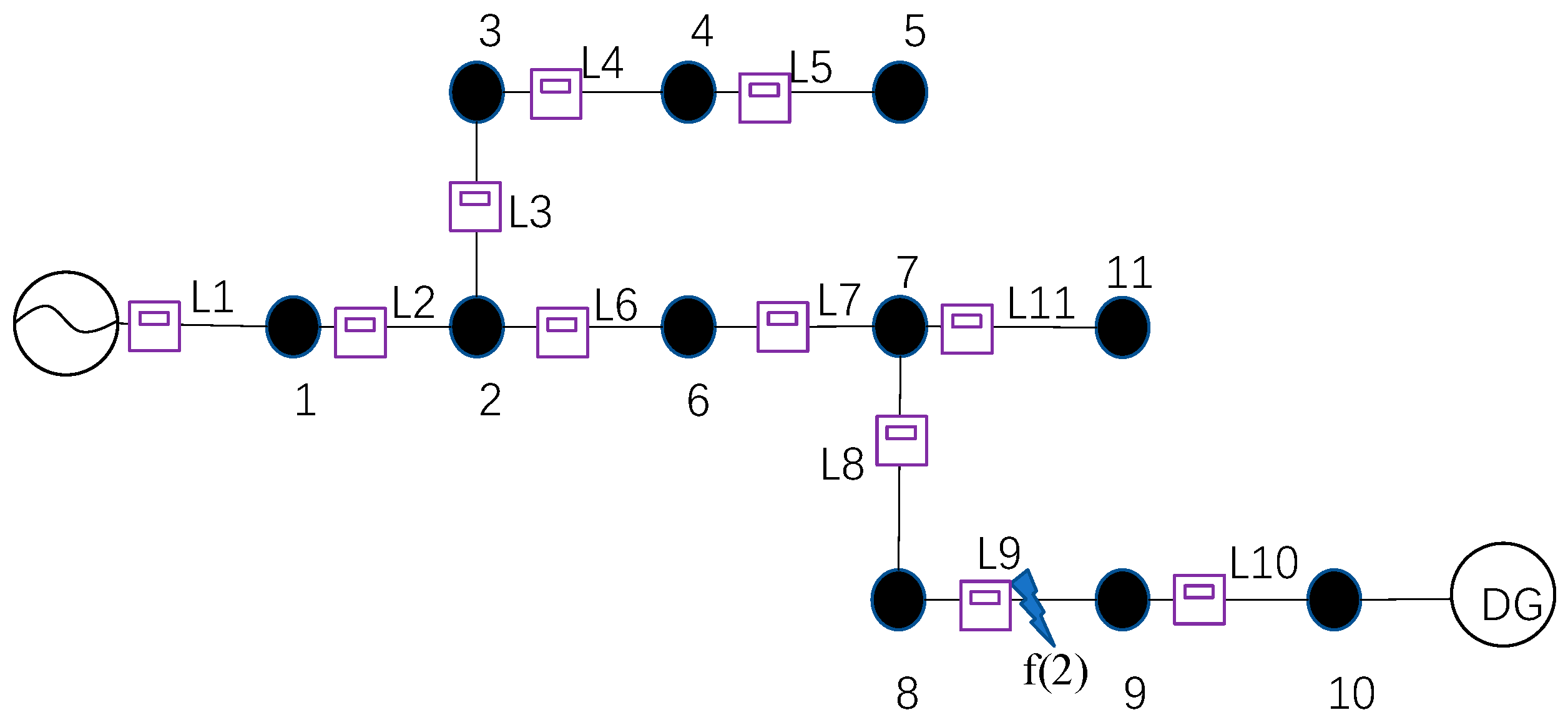
Take the 11-node distribution network in Figure 1 as an example to encode the switching function. In the distribution grid system where both main and distributed power sources have been connected, when a fault occurs in the L9 section, the expected fault current array is obtained from Equation (20), as [1 1 0 0 0 0 1 1 1 1 −1 −1 0].
3.2. Information Perturbation Processing
FTU devices may not be able to transmit fault information to the master station due to perturbations in the information layer, and the possible perturbation of the information subjected to the perturbation needs to be handled in the location algorithms. DCPSs are mainly faced with three types of information perturbations: information distortions, transmission delays, and information failures.
- Information distortion:
Disturbances in the transmission process may cause significant deviations between the value collected by the FTU and the value received by the master station, resulting in information distortion. At this time, the master station can still form a complete fault current array based on the received information. Since the fault feature matching method relies on the highest overall similarity between the actual fault current information characteristics and the expected fault set to achieve fault location, the distortion of some information does not affect the fault information characteristics of the distribution network as a whole, which gives the fault feature matching method a certain degree of anti-disturbance capability. Therefore, there is no need to perform special processing of the distortion information.
- 2.
- Transmission delay:
The transmission delay problem may arise during the uploading of information by the FTU due to fluctuations in the communication network, which may cause the time for the master station to receive the information to exceed the specified maximum delay threshold. The effect of transmission delay on the location method depends on the delay duration. Considering the transmission delay, the message transmission duration T is [21,22]:
where is the base communication time, is the delay time, which usually obeys a Gaussian distribution [22,23], rand(0,1) is the generation of a random number between 0 and 1, int is an integer function, and is the transmission error probability.
When the information transmission time T is less than the maximum specified delay threshold of the system, the master station can receive the FTU acquisition value and form the fault current array within the specified time, which can be regarded as the delay on the algorithm running time having a small impact; when the transmission time is longer than the maximum threshold, the master station cannot receive the corresponding FTU acquisition value within the specified time, which can be regarded as the failure of the information of its faults [5], and at this time, it will be processed according to the failure of the information.
- 3.
- Information failure:
When the FTU fails or the communication link is interrupted, it will lead to the failure of the fault information. At this point, the master SCADA system has the following four processing principles:
- (1)
- When the feeder segment with information failure is located on the system power supply side, report 1 for this lost point information;
- (2)
- When the feeder segment with information failure is located on the distributed power supply side, the loss point information is reported as −1;
- (3)
- When the feeder segment with information failure is located in the middle part of the distribution network and the information of the switch FTUs in two neighbouring positions upstream and downstream is the same, the information of the neighbouring position is used to fill in the missing position information;
- (4)
- When the feeder segment with the failed information is located in the middle part of the distribution network and the switch FTU information of two neighbouring positions upstream and downstream of the switch is not consistent, the system reports the missing point information as 0.
By filling the failed fault information following the above guidelines, the actual fault current array is formed to describe the fault characteristics and matched with the desired fault current array in the predicted fault set to achieve the fault location.
4. Location Method Based on Fault Feature Similarity
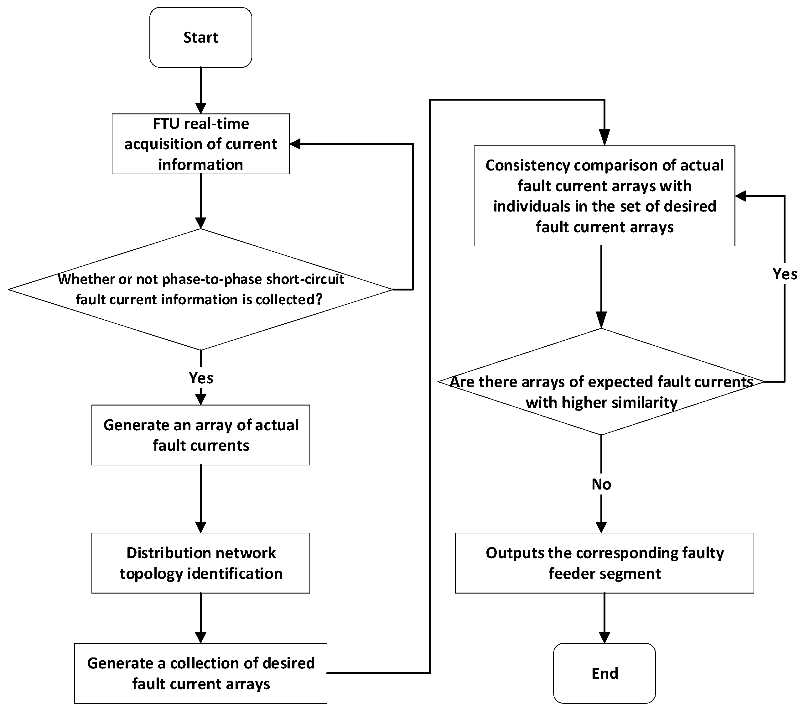
The method of constructing a similarity function to find out the physical layer desired fault current array is consistent with the characteristics of the actual fault current array in the information layer to achieve fault location. The basic flow of fault location method based on similarity of fault features is shown in Figure 2.
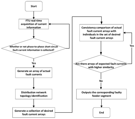
Figure 2.
Block diagram of the basic process of fault location method.
4.1. Construction of Similarity Function
In the case of increasing complexity of distribution network topology, for the same actual fault current array, it can lead to a variety of expected fault arrays corresponding to it making = 0, which leads to an inability to find a suitable expected fault current array, so this paper introduces the statistical term of the number of faulted lines, and the constructed similarity function is shown in Equation (16):
where is the number of nodes in the distribution system, that is the number of FTU, is the actual fault situation fed back from the FTU, i.e., the input term, which is taken as 1 when the overcurrent signal is detected at the th node, otherwise it is taken as 0. is the weight coefficient. indicates the status of the feeder line and is taken as 1 if there is a fault, and 0 if there is no fault. The statistical term of the number of faulty lines plays the role of a penalty function, so as to minimize the difference between the characteristics of the fault information and the expectation value deduced from the switching function corresponding to the fault scenario, and to avoid misjudgement.
4.2. Solution Algorithm
The variational bee colony (VBC) algorithm has the advantage of balancing local and global solution space search [24], which can meet the accuracy and fastness requirements for fault location during distribution network operation.
Each desired fault current array in the expected fault set is treated as an individual, and the dimension of the individual is the number of distribution networks. The population size is reasonably selected according to the specific problem scale and computing resources and generally takes values within the range of [30, 100]. The number of iterations is weighed based on the convergence of the algorithm and computing efficiency, and is usually set between [50, 200] feeder segments, and the solution is realized by finding the individual with the optimal similarity. In the optimization process, the algorithm updates the to-be-selected individuals by roulette, and the probability of an individual being selected is:
From Equation (17), it is known that the higher the value of the adaptation degree, the higher the probability that the individual is selected. After an individual is selected, it exchanges information with a random individual to generate a new individual and selects the original individual and the new individual according to the fitness until the individual with the optimal fitness is selected. In order to avoid falling into local optimization in the solution process, the method of randomly generating new individuals is used, and the operation of forced updating is performed on the individuals to be selected in the iteration, as shown in Equation (18):
where denotes the value of individual a in the dth dimension, and is the upper and lower bound of the solution space, respectively.
At the early stage of iteration, in order to improve the search efficiency, the forced update operation can ensure that the difference between the new individual and the original individual is large, improve the algorithm’s global optimization search performance, and ensure the accuracy of location. As the number of individual dimensions increases, the search space will also increase, and the dynamic variation neighbourhood search strategy is introduced in the late iteration, where the value of each dimension in the individual decides whether or not to be varied according to the variation probability P, and P will decrease with the number of iterations to ensure the convergence speed, as shown in Equation (19):
where is the current iteration number, is the maximum iteration number, , is the variance probability at the beginning of the iteration, and is the variance probability at the end of the iteration.
In this study, the population size of the variational bee colony algorithm is selected as 60 according to the network scale and computing resources. The number of iterations is set to 100, taking into account both the convergence of the algorithm and the computational efficiency. The initial variance probability is set to 0.8, and the final variance probability is set to 0.2, in order to balance the global search ability of the algorithm in the early stage of the search and the local search ability in the later stage.
5. Case Analysis
Analyzing and verifying the effectiveness and applicability of the previously proposed interphase fault location method for distribution networks based on the MATLAB 2021a (MathWork, Natick, MA, USA) platform.
5.1. Analysis of Methodological Validity
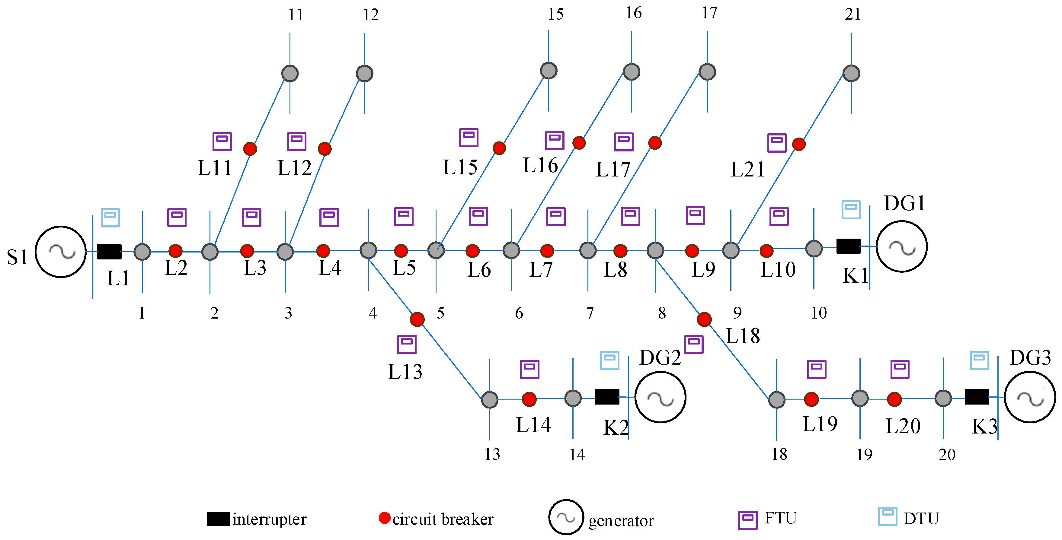
The structure of the 21-node distribution network CPS system at Datan Station, Feng County, Chengde, Hebei Province, is shown in Figure 3, where L1–L21 are 21 feeder segments, 1–21 are 21 nodes, and K1–K3 are the access switches for each distributed power source. The capacity of this system is 300 MW. Distributed power sources are connected to the system through the access switches K1, K2, and K3. K1, K2, and K3 are connected to nodes 10, 20, and 21, respectively. The capacities of the distributed power sources are 30 MW, 70 MW, and 50 MW, respectively.
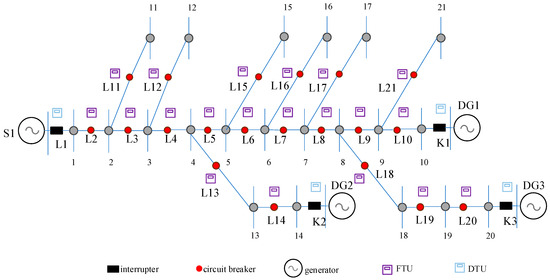
Figure 3.
21-nodes distribution grid CPS system structure at Datan Station, Feng County, Chengde, Hebei, China.
In this study, the fault current discrimination coefficient is set to 1.3, and the number of sampling points in one cycle is set to 128. These parameter values are determined based on a large number of preliminary experiments and practical engineering experience. They can not only ensure the accurate extraction of fault current characteristics but also effectively balance the computational load and positioning accuracy.
In the following simulation, the location accuracy, the average number of converged generations, and the iteration time are used as the algorithm performance evaluation indexes, and the method of this paper is adopted for the location of single-point and multi-point faults, as well as interphase faults, in the scenarios of information perturbation.
- 1.
- Unperturbed information scenarios:
In order to simulate the distributed power supply access to the distribution network in different numbers and locations, eight classifications are made for single-point and multi-point fault location simulations, and the distributed power supply access switches K1, K2, K3 in state 1 indicate that the distributed power supply accesses the system, and the opposite is true when the state 0 is the case. The simulation experiment results are shown in Table 1.

Table 1.
Experimental results of fault location simulation.
From the data in Table 1, it can be seen that the algorithm proposed in this paper can accurately and quickly locate single-point and multi-point faults in the case of different numbers and locations of distributed power sources connected to the distribution network.
When the total number of faulty lines is set to 2 in the situation [0,1,1], the calculation time is relatively long. This may be due to the fact that the connection locations and state changes of distributed generators lead to a more complex distribution of power flow in the network. When the connection locations and states of distributed generators change, they will affect the magnitude and direction of the fault current and further influence the construction of the expected fault set in the physical layer and the processing procedure of the fault current information in the information layer in the fault location algorithm. In such a case, the algorithm requires more computing resources and time to accurately match the fault characteristics of the physical layer and the information layer, thus resulting in an increase in the calculation time.
- 2.
- Perturbed information scenarios:
Based on the processing method of coping with fault information perturbation in the previous section, the scenario of fault information failure is set up in the simulation model, and the effectiveness of the method is analyzed. According to the GB/T 42151.5-2022 Chinese power automation communication network and system standard [25], the range of faults in the information layer of the CPS of the current electric power system can generally not exceed 25% of the communication nodes, and therefore, the feeder segments in the simulation set up to have information perturbed number does not exceed 25% of the total number, that is 5.
- (1)
- Information distortion:
The simulation results for the information distortion case are shown in Table 2.
Table 2.
Experimental results of simulation under information distortion.
- (2)
- Information delay:
The results of the simulation experiments under the occurrence of information delay are shown in Table 3.
Table 3.
Results of simulation experiments under information delay.
- (3)
- Information failure:
The results of the simulation experiments in cases of information failure are shown in Table 4.
Table 4.
Results of simulation experiments under information failure.
As can be seen from these tables, in various types of information perturbation scenarios, the location method still remains more effective, the location accuracy remains above 92%, and the algorithm computation time is basically stable within 3 s.
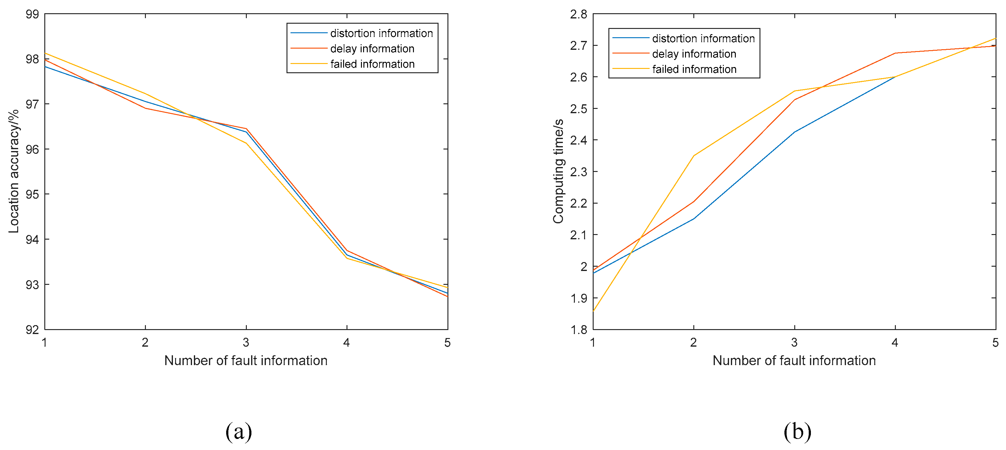
Figure 4 provides a visual representation of the fault location accuracy and computing time under different information fault conditions.
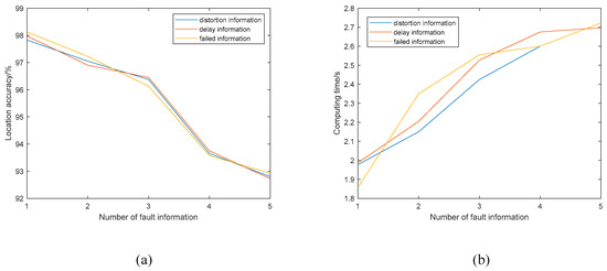
Figure 4.
(a)The accuracy rate of fault location under different information fault conditions. (b) The computing time under different information fault conditions.
From Figure 4, we can clearly observe the following statistical trends:
Information Distortion: As the number of distorted information increases, the fault location accuracy gradually decreases. For instance, when there is 1 distorted information, the accuracy is 98.7%, and it drops to 92.1% when the number of distorted information reaches 5. This indicates that although the fault feature matching method has a certain degree of anti-disturbance ability, a higher level of information distortion still has a negative impact on the accuracy.
Information Delay: The impact of information delay on the fault location accuracy is relatively milder compared to distortion. With the increase in the number of delayed information, the accuracy shows a slow downward trend. When there is 1 delayed information, the accuracy is 98.4%, and it reduces to 92.2% when there are 5 delayed information. The computing time also increases slightly, but the overall algorithm performance remains relatively stable.
Information Failure: Similar to information distortion, the increase in the number of failed information leads to a decline in the fault location accuracy. When 1 piece of information fails, the accuracy is 98.9%, and it decreases to 92.4% when 5 pieces of information fail. This shows that information failure has a significant influence on the accuracy, and our proposed method’s ability to handle information failure is also an important factor in ensuring reliable fault location.
By presenting these statistical analyses, we have provided a more in—depth understanding of how different types of information perturbations affect the performance of our fault location method. This not only validates the effectiveness of our proposed approach but also highlights its limitations in the face of information—related challenges. We believe that these findings contribute to a more comprehensive assessment of the proposed method and are valuable for further research and improvement in the field of distribution network fault location.
5.2. Analysis of Methodological Applicability
In order to verify the adaptability of the algorithm proposed in this paper in the face of different system network topologies, simulation experiments were carried out using the IEEE-33 node system as an example. The algorithm location accuracy and runtime were counted for various scenarios where the topology of the IEEE-33 node system may change [26], and the average results of the accuracy and runtime for each topology are shown in Table 5.
Table 5.
Experimental results of simulation with topology changes.
As can be seen from Table 5, the algorithm exhibits good performance under the topology change of the distribution network, with the location accuracy remaining above 97% and the computation time stabilized within 2 s.
In order to verify the impact of system-scale expansion on the effectiveness of the method, IEEE-9 [27], IEEE-33 [28], and IEEE-160 [29], three different sizes of distribution network arithmetic examples, were used to analyze the applicability of the method under the different sizes of the system, and the results are shown in Table 6.
Table 6.
Experimental results of algorithm simulation under different scale cases.
As can be seen from Table 6, as the system size increases, the computation time of the fault location method increases, but the accuracy of the method is still above 94% and the computation speed is faster, and the proposed method has the advantage of both accuracy and speed.
In addition, fault location algorithms based on the immune algorithm (IA), genetic algorithm (GA), quantum genetic algorithm (QGA), binary dragonfly algorithm (BDA), and slime mould algorithm (SM) are selected for comparison with the algorithm of this paper, and the performance evaluation indexes of the statistical location algorithms are evaluated in cases of different numbers and locations of distributed power sources accessing the distribution network, and the results are shown in Table 7.
Table 7.
Comparison of different algorithms.
Through comparative analysis with other optimization algorithms, it can be seen that: compared with traditional intelligent algorithms such as IA and GA, the improved VBC algorithm with adaptive weights has a higher population quality and better positioning accuracy.
In terms of local search ability, the immune algorithm (IA) is mainly based on the principles of the biological immune system, seeking the optimal solution through the matching of antibodies and antigens. When faced with complex distribution network fault location problems, the update and selection mechanism of IA’s immune memory cells is relatively fixed, which limits its ability to search for better solutions in local areas. When the algorithm becomes trapped in a local optimum, it is difficult to quickly jump out and explore other potentially better regions. For example, when dealing with some complex fault characteristics, IA may be unable to adjust the search direction in a timely manner due to excessive reliance on existing immune memory, thus missing the true fault location.
The genetic algorithm (GA), on the other hand, simulates the natural genetic evolution process and iteratively optimizes the population through selection, crossover, and mutation operations. In the GA, although crossover and mutation operations can introduce new solution spaces, these operations are somewhat random. In distribution network fault location, this randomness may prevent in-depth exploration of the neighbourhood of the current optimal solution during a local search. When there are multiple similar local optimal solutions in the solution space near the fault location, GA may wander among these local optimal solutions, making it difficult to quickly find the global optimal solution, thereby affecting the accuracy and efficiency of fault location.
In contrast, the variational bee colony (VBC) algorithm proposed in this paper has unique advantages in local search. In the later stage of iteration, VBC introduces a dynamic variable neighbourhood search strategy. This strategy decides whether to change the dimension according to the individual dimension value and the change probability P, and P decreases with the increase in the number of iterations. When approaching the optimal solution, a smaller P value enables the algorithm to search the local area more precisely. For example, when the algorithm gradually approaches the optimal solution of the fault location, the dynamic variable neighbourhood search strategy can adjust the search direction in a targeted manner according to the current individual state, and conduct a more detailed evaluation of the solutions in the neighbourhood, thus being more likely to find the global optimal solution and avoiding missing the true fault location.
In terms of iteration speed, when dealing with complex problems, due to the complexity of its immune calculations, the update and selection mechanism of immune memory cells in the immune algorithm (IA) may lead to an increase in computational complexity, thus affecting the iteration speed. During the process of distribution network fault location, a large amount of fault data and complex network structures need to be processed. The computational characteristics of IA make its iteration process slow and unable to meet the requirement of quickly locating faults.
Although the crossover and mutation operations of the genetic algorithm (GA) can bring diversity, they may also cause deviations in the search direction. In each iteration, crossover and mutation operations randomly generate new individuals, which may cause the algorithm to take some detours during the search process and increase unnecessary iteration times. In distribution network fault location, it is crucial to quickly and accurately find the fault location. This characteristic of GA may delay the fault location time and affect the normal operation of the power system.
The variational bee colony (VBC) algorithm, however, adopts a forced update operation in the early stage of iteration. This operation ensures that the new individual is significantly different from the original individual, enabling quick exploration of different regions in the solution space, improving the global search efficiency, and rapidly narrowing the search range. For example, when facing large-scale distribution network fault location problems, the VBC algorithm can quickly identify the areas where faults may exist through the forced update operation, laying a foundation for subsequent precise searches. As the iteration progresses, the VBC algorithm gradually adjusts its search strategy, enhancing the local search ability while maintaining the global search ability so that the algorithm achieves a better balance between iteration speed and location accuracy.
In summary, in terms of both local search ability and iteration speed, the variational bee colony (VBC) algorithm proposed in this paper has obvious advantages over the immune algorithm (IA) and the genetic algorithm (GA) and can locate distribution network faults more quickly and accurately.
Compared with the QGA, the two have similar optimization capabilities, but the improved VBC algorithm has stronger local exploration ability and shorter iteration time, ensuring the rapidity of positioning. In addition, it is found that when a fault occurs in the S1 feeder section, more advanced artificial intelligence algorithms, such as BDA and SM, may have inaccurate positioning. The analysis of the reasons shows that because the fault point is close to the power source, the occurrence of the fault will cause a huge change in the overall power flow of the distribution network, and the current characteristic information of the distribution network before and after the fault is very different. However, in the BDA and SM, it is difficult to consider similar extreme situations when generating the candidate population, resulting in positioning deviations. The improved VBC algorithm is similar to them in iteration speed but has better positioning accuracy and is more suitable for fault location algorithms.
6. Conclusions
In this paper, a novel interphase short-circuit fault location method for distribution networks was proposed, taking into account the topology flexibility and information perturbation. This research contributes to the field of power systems with several distinct scientific innovations.
The first innovation lies in the integration of multiple key elements. By integrating distribution network topology identification, the construction of a switching function based on interphase short-circuit fault current characteristics, and the handling of information perturbations, a comprehensive and adaptable fault location framework is established. This integrated approach is designed to address the complex and dynamic nature of modern distribution networks, where traditional methods often fall short.
Secondly, the construction of similarity functions for fault features across physical and information layers, in conjunction with the application of the variational bee colony algorithm, represents a significant leap forward. The variational bee colony algorithm exhibits remarkable advantages in balancing local and global search spaces. Compared with traditional algorithms such as the immune algorithm (IA) and genetic algorithm (GA), it showcases superior local exploration capabilities and faster iteration speeds. This enables the algorithm to more efficiently match the actual fault current array with the expected ones, resulting in highly precise fault location outcomes.
Furthermore, comprehensive strategies have been developed to manage various information perturbations, including distortion, delay, and failure. These strategies are essential for enhancing the fault tolerance of the fault location method, ensuring its reliable performance even in the face of imperfect or disrupted information flow.
Subsequently, an anticipatory fault set construction method considering distribution network topology identification was presented. This method is well-suited to the intricate and flexible topologies of contemporary distribution networks. Additionally, a fault current information feature modelling approach was introduced, which accounts for the impacts of information perturbations such as distortion, transmission delay, and information failure. Finally, similarity functions for fault features in physical and information layers were constructed, and a fault location method for distribution networks was proposed, which effectively improves the fault tolerance to information perturbation.
The effectiveness of the proposed methods has been thoroughly verified through analyses. The results indicate that these methods are fast, accurate, and fault-tolerant across distribution networks of varying scales. Simulation studies based on real-world projects in Hebei and the IEEE system have demonstrated that the proposed method achieves high location accuracy, short computing times, and strong adaptability to diverse fault scenarios. These scenarios encompass single-point and multi-point faults, dynamic topology changes, and information perturbations.
Looking ahead, the authors intend to conduct in-depth research on fault isolation methods for distribution network cyber–physical systems (CPS) in the presence of information perturbations. The goal of this future work will be to further reduce fault losses and enhance the overall reliability and safety of distribution networks. This subsequent research will build upon the solid foundation established by the fault location method proposed in this study, thereby contributing to the continuous development and improvement of power system operation and management.
Author Contributions
Conceptualization, H.X. and Z.L.; methodology, H.X.; software, Z.L.; validation, Q.C., C.Y. and T.L.; formal analysis, K.L.; investigation, K.L.; data curation, K.L.; writing—original draft preparation, Z.L.; writing—review and editing, K.L.; visualization, Z.L.; supervision, H.X.; project administration, Q.C.; funding acquisition, C.Y. and T.L All authors have read and agreed to the published version of the manuscript.
Funding
This research was funded by National Key Research and Development Programme, grant number 2022YFB3105100.
Data Availability Statement
The original contributions presented in the study are included in the article further inquiries can be directed to the corresponding author.
Conflicts of Interest
Authors Yang and Tong Li were employed by State Grid Liaoning Electric Power Supply Co., Ltd. The remaining authors declare that the research was conducted in the absence of any commercial or financial relationships that could be construed as a potential conflict of interest.
References
- Bango, O.; Misra, S.; Jonathan, O.; Ahuja, R. Power system protection on smart grid monitoring faults in the distribution network via IoT. In New Frontiers in Cloud Computing and Internet of Things; Springer: Berlin/Heidelberg, Germany, 2022; pp. 343–363. [Google Scholar]
- Qin, J.; Yu, D.; Wang, H. Research on distribution network monitoring and fault location based on edge computing. Water Lect. Notes Electr. Eng. 2024, 1132, 260–265. [Google Scholar]
- Zhang, C.; Liu, Z.; Wang, J.; Wang, Z. Fast fault detection and location system for distribution network lines based on power electronic disturbance signals. J. Circuits Syst. Comput. 2021, 30, 2150187. [Google Scholar] [CrossRef]
- Ma, T.; Hu, Z.; Xu, Y.; Dong, H. Fault location based on comprehensive grey correlation degree analysis for flexible DC distribution network. Energies 2022, 15, 7820. [Google Scholar] [CrossRef]
- An, D.; Zhang, F.; Cui, F.; Yang, Q. Toward data integrity attacks against distributed dynamic state estimation in smart grid. IEEE Trans. Autom. Sci. Eng. 2024, 21, 881–894. [Google Scholar]
- Huang, C.; He, H.; Wang, Y.; Miao, R.; Ke, Z.; Chen, K. Low-voltage characteristic voltage based fault distance estimation method of distribution network. Front. Energy Res. 2024, 12, 1357459. [Google Scholar] [CrossRef]
- Ngoc-Hung, T. A new method for estimating fault location in radial medium voltage distribution network only using measurements at feeder beginning. Arch. Electr. Eng. 2023, 72, 503–520. [Google Scholar]
- Shu, H.; Liu, X.; Tan, X. Single-ended fault location for hybrid feeders based on charaeterislie distribution of traveling wave along a line. IEEE Trans. Power Deliv. 2021, 36, 339–351. [Google Scholar] [CrossRef]
- Li, L.; Gao, H.; Yuan, T.; Peng, F.; Xue, Y. Location method of high-impedance fault based on transient zero-sequence factor in non-effectively grounded distribution network. Electr. Power Syst. Res. 2024, 226, 109912. [Google Scholar] [CrossRef]
- Zhang, Z.; Huang, S.; Chen, Y.; Li, B.; Mei, S. Cyber-physical coordinated risk mitigation in smart grids based on attack-defense game. IEEE Trans. Power Syst. 2022, 37, 530–542. [Google Scholar] [CrossRef]
- Sun, Y.; Chen, Q.; Xie, D.; Shao, N.; Ding, W.; Dong, Y. Novel faulted-section location method for active distribution networks of new-type power systems. Appl. Sci. 2023, 13, 8521. [Google Scholar] [CrossRef]
- An, J.; Deng, Z.; Chen, H.; Mu, G. Fault location detection of transmission lines in noise environments based on random matrix theory. CSEE J. Power Energy Syst. 2022, 8, 1233–1241. [Google Scholar]
- Liu, Z.; Chen, K.; Xie, J.; Wu, X.; Lu, W. Active distribution network fault section location method based on characteristic wave coupling. IET Renew. Power Gener. 2024, 18, 3020–3039. [Google Scholar] [CrossRef]
- Wang, S.; Zhao, K. Fault location of distribution network with distributed generation based on Karrenbauer transform and support vector machine regression. Arch. Electr. Eng. 2023, 72, 461–481. [Google Scholar]
- Wang, D.; Yu, D.; Gao, H.; Peng, F.; Lin, J.; Wang, J. Frequency modification algorithm-based traveling wave fault location approach for overhead transmission lines with structural changes. Prot. Control of Mod. Power Syst. 2025, 10, 1–12. [Google Scholar] [CrossRef]
- Kanwal, S.; Jiriwibhakorn, S. Artificial intelligence based faults identification, classification, and localization techniques in transmission lines-a review. IEEE Lat. Am. Trans. 2024, 21, 1291–1305. [Google Scholar] [CrossRef]
- Niu, S.; Zhao, Q.; Niu, S.; Jian, L. A comprehensive investigation of thermal risks in wireless EV chargers considering spatial misalignment from a dynamic perspective. IEEE J. Emerg. Sel. Top. Ind. Electron. 2024, 4, 1560–1571. [Google Scholar] [CrossRef]
- Azizivahed, A.; Arefi, A.; Ghavidel, S.; Shafie-khah, M.; Li, L.; Zhang, J.; Catalao, J. Energy management strategy in dynamic distribution network reconfiguration considering renewable energy resources and storage. IEEE Trans. Sustain. Energy 2020, 11, 662–673. [Google Scholar] [CrossRef]
- Fan, B.; Shu, N.; Li, Z.; Li, F. Critical nodes identification for power grid based on electrical topology and power flow distribution. IEEE Syst. J. 2023, 17, 4874–4884. [Google Scholar] [CrossRef]
- Wang, H.; Gu, C.; Zhao, W.; Wang, S.; Zhang, X.; Buticchi, G.; Gerada, C.; Zhang, H. Fault-tolerant control for single-phase open-circuit and short-circuit fault in five-phase PMSM with third-order harmonic back EMF using coefficients reconfiguration. IEEE Trans. Energy Convers. 2024, 39–51, 782–792. [Google Scholar] [CrossRef]
- Gutierrez-Rojas, D.; Christou, I.; Dantas, D.; Narayanan, A.; Nardelli, P.; Yang, Y. Performance evaluation of machine learning for fault selection in power transmission lines. Knowl. Inf. Syst. 2022, 64, 859–883. [Google Scholar] [CrossRef]
- Zhang, G.; Zhao, J.; Ma, Z.; Chen, J.; Ren, H. A fault recovery strategy for distribution networks considering distributed energy storage and information systems. In Proceedings of the 11th Frontier Academic Forum of Electrical Engineering (FAFEE2024), Chongqing, China, 21 June 2024. [Google Scholar]
- Samal, S.; Samantaray, S. A novel sequence component based fault detection index for microgrid protection. Electr. Power Syst. Res. 2024, 232, 110380. [Google Scholar] [CrossRef]
- Das, C.; Bass, O.; Kothapalli, G.; Mahmoud, T.; Habibi, D. Optimal placement of distributed energy storage systems in distribution networks using artificial bee colony algorithm. Appl. Energy 2018, 232, 212–228. [Google Scholar] [CrossRef]
- GB/T 42151.5-2022; Communication Networks and Systems for Power Utility Automation—Part 5: Communication Requirements for Functions and Device Models. Standardization Administration of China: Beijing, China, 2022.
- Liu, B.; Chen, J.; Li, J. Distribution network topology identification method based on state estimation with mixed integer programming and structural equation model. Int. J. Electr. Power Energy Syst. 2024, 162, 110251. [Google Scholar] [CrossRef]
- Xu, H.; Feng, B.; Wang, C.; Guo, C.; Qiu, J.; Sun, M. Exact box-constrained economic operating region for power grids considering renewable energy sources. J. Mod. Power Syst. Clean Energy 2024, 12, 514–523. [Google Scholar] [CrossRef]
- Xu, D.; Wu, Z.; Xu, J.; Hu, Q. Data-Model Hybrid Driven Topology Identification Framework for Distribution Networks. CSEE J. Power Energy Syst. 2024, 10, 1478–1490. [Google Scholar]
- Sheng, W.; Liu, K.; Li, Z.; Ye, X. Collaborative fault recovery and network reconstruction method for cyber-physical-systems based on double layer optimization. CSEE J. Power Energy Syst. 2023, 9, 380–392. [Google Scholar]
Disclaimer/Publisher’s Note: The statements, opinions and data contained in all publications are solely those of the individual author(s) and contributor(s) and not of MDPI and/or the editor(s). MDPI and/or the editor(s) disclaim responsibility for any injury to people or property resulting from any ideas, methods, instructions or products referred to in the content. |
© 2025 by the authors. Licensee MDPI, Basel, Switzerland. This article is an open access article distributed under the terms and conditions of the Creative Commons Attribution (CC BY) license (https://creativecommons.org/licenses/by/4.0/).