Optimized Dispatch of Integrated Energy Systems in Parks Considering P2G-CCS-CHP Synergy Under Renewable Energy Uncertainty

Abstract

To enhance low-carbon economies within Park Integrated Energy Systems (PIES) while addressing the variability of wind power generation, an innovative optimization scheduling strategy is proposed, incorporating a reward-and-punishment ladder carbon trading mechanism. This method effectively mitigates the unpredictability of wind power output and integrates Power-to-Gas (P2G), Carbon Capture and Storage (CCS), and Combined Heat and Power (CHP) systems. This study develops a CHP model that combines P2G and CCS, focusing on electric-heat coupling characteristics and establishing constraints on P2G capacity, thereby significantly enhancing electric energy flexibility and reducing carbon emissions. The carbon allowance trading strategy is refined through the integration of reward and punishment coefficients, yielding a more effective trading model. To accurately capture wind power uncertainty, the research employs kernel density estimation and Copula theory to create a representative sequence of daily wind and photovoltaic power scenarios. The Dung Beetle Optimization (DBO) algorithm, augmented by Non-Dominated Sorting (NSDBO), is utilized to solve the resulting multi-objective model. Simulation results indicate that the proposed strategy increases the utilization rates of renewable energy in PIES by 28.86% and 19.85%, while achieving a reduction in total carbon emissions by 77.65% and a decrease in overall costs by 36.91%.

1. Introduction

Integrated energy systems offer numerous benefits, including enhanced energy efficiency, improved reliability of energy supply, and support for the development of smart grid infrastructure. However, they also represent significant sources of global carbon emissions. In the context of escalating concerns regarding global warming and ecological degradation, PIES present an important avenue for exploring pathways toward low-carbon, economically viable, and reliable energy operations.

Among these pathways, energy substitution is vital for meeting global carbon reduction goals [1]. In recent years, the capacity for wind and solar photovoltaic energy has consistently increased, leading to a notable decline in fossil fuel consumption and associated carbon emissions. However, the intermittent and variable characteristics of wind and solar energy create challenges in power scheduling, often resulting in the curtailment of renewable generation as their capacities grow in many areas [2]. Sinha et al. observed a growing trend of mixed energy systems that combine solar photovoltaic and wind energy, indicating a promising direction for the evolution of energy systems [3]. Zhao et al. designed a topological framework for a hybrid power generation system that integrates wind, solar, and hydro sources, focusing on minimizing energy curtailment and addressing economic factors; however, their model did not account for the uncertainties inherent in wind and solar outputs or the resultant carbon emissions [4]. Ju et al. indicated that properly managing the uncertainties associated with wind and solar energy production can bolster the reliability, stability, and economic viability of integrated energy systems [5]. Liu et al. demonstrated that effective scheduling within these systems facilitates smoother transitions between various energy sources, thus enhancing the utilization of renewable resources like wind and solar energy [6]. Xu et al. introduced a martingale model to assess the uncertainties in wind and photovoltaic energy outputs; nonetheless, this method faced challenges due to its randomness and subjectivity in selecting representative scenarios [7]. In a study by Min, a cloud model combined with a copula correlation coefficient matrix was utilized to analyze a hybrid power generation system based on output data. This approach successfully assessed the correlation and uncertainty of wind and solar outputs; however, obtaining the necessary data for its implementation may prove difficult in practical scenarios [8]. However, there are few existing articles that simultaneously consider the uncertainty and correlation of wind and solar power output, and they do not accurately depict the typical daily values of wind and solar power output, lacking a detailed mathematical modeling process. This research aims to improve upon this aspect.

In the context of low-carbon economic optimization strategies for PIES, researchers worldwide have explored the integration of carbon trading mechanisms and voluntary emission reductions into carbon emission policies. Chen et al. presented carbon emission limits and renewable energy integration targets within PIES, highlighting potential synergies between low-carbon goals and renewable energy consumption objectives [9]. Zhang et al. developed an optimized scheduling model for PIES that incorporates a tiered carbon trading mechanism and addresses the uncertainty of wind and solar generation. Their findings demonstrated the model’s advantages in terms of both low-carbon outcomes and economic performance, although they overlooked the complementary dynamic between wind and solar energy [10]. Zhu et al. introduced a comprehensive trading approach within PIES focusing on carbon constraints. This method advocates for spot trading of excess industrial energy and the use of storage solutions to manage energy supply and demand variations, thus easing carbon emission pressures. Case studies confirmed that this approach can enhance economic returns while lowering carbon emissions [11]. Liu et al. observed that the rapid growth of the hydrogen energy sector is increasing hydrogen’s share in energy systems, complicating the conversion among energy sources and posing challenges for PIES planning and development. To tackle this, they proposed a bi-level planning model for a hydrogen-integrated energy system that considers multi-stage investments and carbon trading. Simulation results suggested that this model could effectively reduce operational costs and carbon emissions within the PIES planning framework [12]. Zhang et al. designed a tiered carbon trading model that accounts for complete lifecycle carbon emissions to study the influence of carbon trading on PIES, illustrating that detailed modeling of specific equipment and hydrogen blending processes can contribute to emission reductions [13]. Li et al. put forth an electric-carbon energy scheduling approach for multi-park integrated energy systems (MIESs), establishing a joint electric-carbon trading market to facilitate energy interactions among multiple integrated energy systems. This strategy leverages regional differences in carbon pricing, allowing for the sharing of carbon quotas among systems and ultimately lowering overall carbon trading costs [14]. The studies mentioned demonstrate significant progress in modeling and optimizing PIES with a focus on carbon emissions. Implementing multi-energy coupling, flexible demand responses, and enhanced energy allocation mechanisms within parks can also provide low-carbon economic benefits. Chen et al. suggested a joint planning and cost allocation method for multi-park shared energy systems to develop optimal strategies for joint planning and cost distribution regarding shared storage at the park level [15]. Additionally, Chen et al. introduced a low-carbon integrated energy system that utilizes distributed renewable and clean energy, applying the Firefly algorithm to address constraint conditions [16]. To address the complexities of joint scheduling among industrial, commercial, and residential parks with various energy-sharing modes, Wang et al. established a cooperative game model for multi-park integrated energy systems with hydrogen energy, based on Nash bargaining theory [17]. Xu et al. proposed a multi-objective operational optimization model for an electric and thermal integrated energy system, considering power-to-gas transitions and demand response strategies from different electric and thermal loads, aiming to minimize total costs, carbon emissions, and energy waste rates [18]. The existing research mainly explores the energy-saving and low-carbon operation mode of integrated energy systems from two aspects: multi-energy coupling and equipment joint operation. In terms of multi-energy coupling, the existing research on the relationship between electric energy and thermal energy is constrained by “determining electricity by heat. “The range of electric energy regulation is insufficient, and the effect of cost-saving and carbon emission control is not significant. It is urgent to break this constraint. In terms of equipment joint operation, Ding et al. have proved the advantages of P2G-CCS-CHP joint operation in terms of economy and low carbon in engineering modeling, but there are few applications in the field of optimal scheduling of park-level integrated energy systems [19]. At the same time, the traditional step-by-step carbon trading mechanism commonly used in existing research has been proved to have limited carbon emission constraints in practical applications, and it is necessary to explore more effective carbon emission control methods.

Based on the detailed engineering modeling of Ding et al. [19], this study established the core framework of PIES and coupled the P2G-CCS and CHP systems to effectively solve the CHP-related ‘thermally driven power’ challenge. Limited by space, some unspecified parameter values, system dynamics principles, and internal relations can refer to Ding et al.’s original text. The model collaborates with micro gas turbines (MT) to enable flexible multi-energy responses. Additionally, it features a tiered carbon trading mechanism based on rewards and penalties, accounting for the uncertainties linked to wind and solar energy outputs. The optimization process employs the Dung Beetle Optimizer (DBO) after refining the objective function through the Non-dominated Sorting Genetic Strategy (NSGS). The primary goal of the model is to minimize both operational and environmental protection costs, comparing four different solution strategies: minimizing operational costs, minimizing environmental protection costs, minimizing total costs, and deriving a compromise solution. Furthermore, the study examines the implications of the reward-and-penalty carbon trading mechanism, as well as the uncertainties and correlations present in wind and solar energy sources. It also assesses the roles of P2G, CCS, and CHP technologies in real-world engineering contexts, where total cost minimization is typically a priority. Additionally, the research analyzes how variations in the reward-and-penalty coefficients within the carbon trading framework influence the optimized scheduling of PIES, validating the proposed model’s effectiveness through comparative analysis across various operational scenarios.

2. Methods and Analysis

2.1. Integrated Energy System Framework of the Park with Reward-and-Penalty Tiered Carbon Trading Mechanism

The PIES structure constructed in this study is illustrated in Figure 1. This system comprises three energy networks: electricity, heat, and gas. It includes the main power grid, natural gas sources (NS), wind turbines (WT), photovoltaic power generation (PV) units, P2G-CCS-CHP coupled production units, electric refrigerators (ER), power-to-gas devices (P2G), natural gas energy storage (GasS), gas turbines (GT), gas boilers (GB), organic Rankine cycle (ORC), hydrogen fuel cells (HFC), waste heat boilers (WHB), electric energy storage (ES), and thermal energy storage (hS).

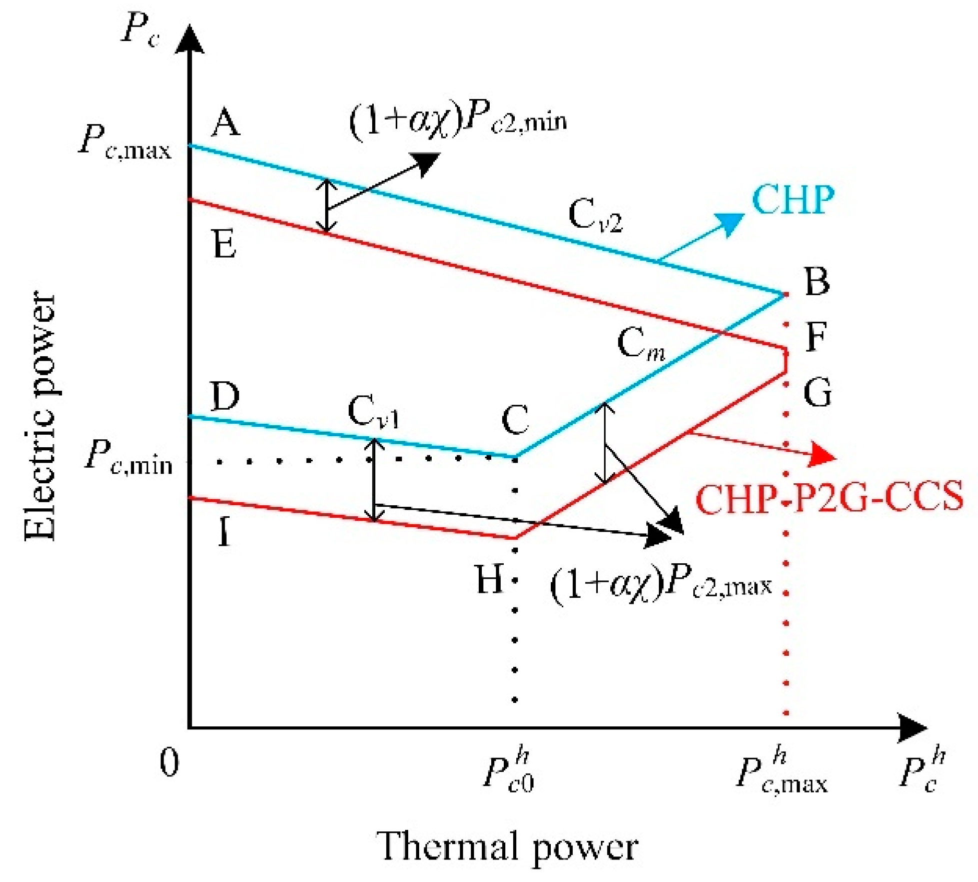
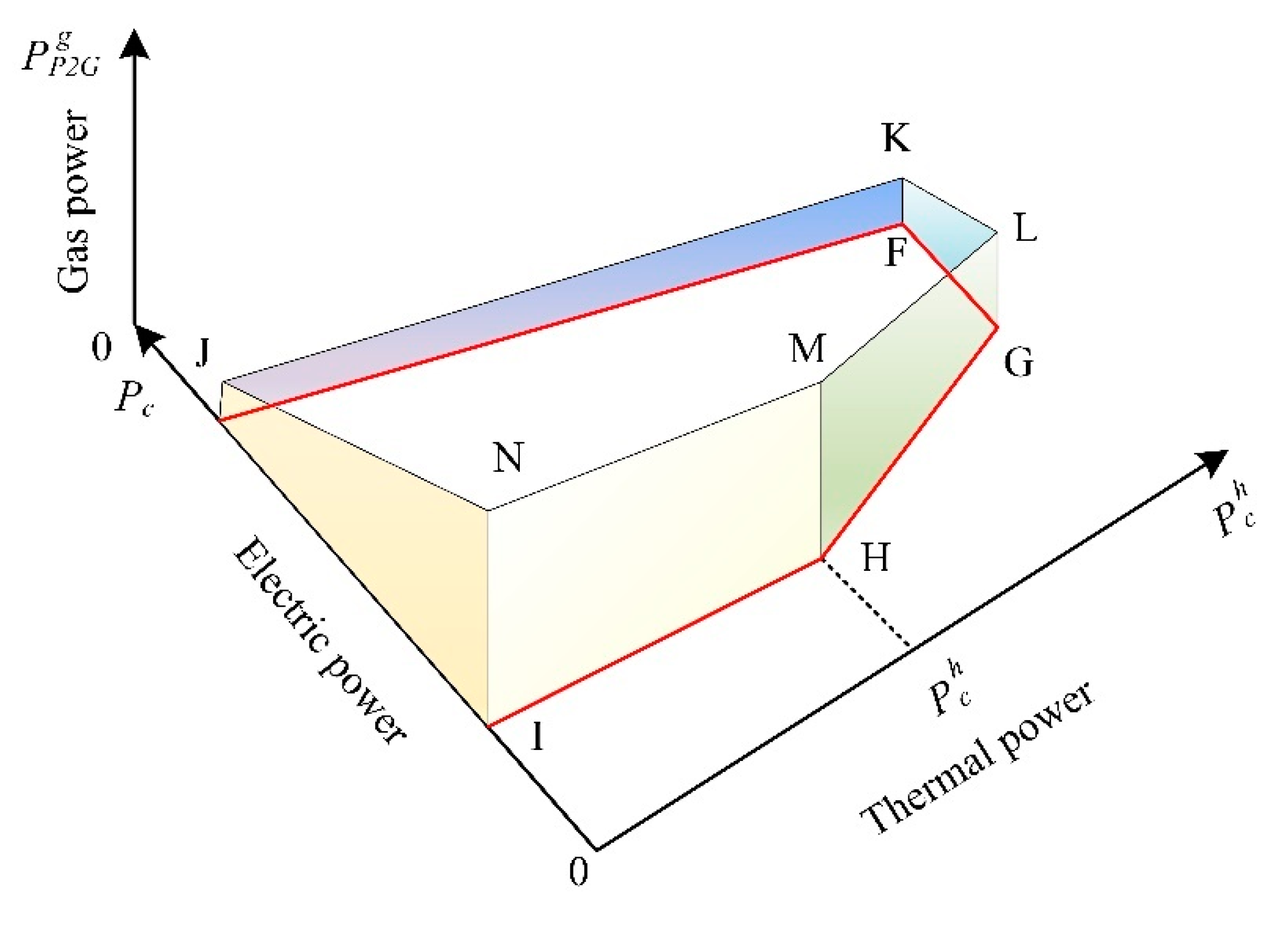
2.1.1. Modeling and Characteristics of P2G-CCS-CHP

To mitigate carbon emissions and reduce transportation costs linked to carbon, this study introduces a coupled operational system that integrates CHP, P2G, and CCS. In this setup, the CHP system produces both electricity and thermal energy using natural gas. The P2G component utilizes electricity from the CHP unit while receiving CO₂ from an adjacent CCS facility. This electricity allows for the conversion of CO₂ into methane, which fulfills the energy requirements of both CHP and gas loads, effectively contributing to emission reduction and enhanced energy efficiency. The CCS system captures CO₂ generated by the CHP process and uses electricity to transport the captured CO2 to the P2G system for reuse as fuel. The close proximity of the CCS and P2G components within the P2G-CCS-CHP system minimizes the need for long-distance transportation and storage of CO₂, thus reducing related costs.

Electricity produced by the CHP system can be utilized in three main ways: it can be directly consumed by end-users via the power grid, delivered to the P2G system for methane production, or sent to the CCS system to facilitate CO₂ management. This can be illustrated as follows:

$$P_c\left(t\right)=P_{c1}\left(t\right)+P_{c2}\left(t\right)+P_{c3}\left(t\right)$$

(1)

where: $t$ represents time, $P_c$ denotes the electricity generated by the CHP system, $P_{c1}$ refers to the total electricity output, $P_{c2}$ signifies the electricity used by the P2G system, and $P_{c3}$ indicates the electricity utilized by the CCS system. The CCS system captures CO₂ through its electricity consumption, with the quantity of CO₂ captured being roughly proportional to the electricity used, expressed as:

$$C_{CCS}\left(t\right)=\alpha P_{c3}\left(t\right)$$

(2)

where: $C_{CCS}$ signifies the quantity of CO₂ captured by the CCS system, and α indicates the capture efficiency, which is a dynamically variable numerical quantity.

The CO₂ collected by the CCS is subsequently transported to P2G for the production of natural gas. The volume of natural gas generated by P2G is roughly proportional to both the quantity of CO₂ utilized and the electrical energy consumed throughout the production process, which can be represented as:

$$P_{P2G}^g\left(t\right)=\beta C_{CCS}\left(t\right)$$

(3)

$$P_{c2}\left(t\right)=\chi C_{CCS}\left(t\right)$$

(4)

where: β and χ are the proportionality coefficients.

Based on Formulas (2) and (4), Formula (1) can be rewritten as:

$$P_c\left(t\right)=P_{c1}\left(t\right)+\left(1+\alpha \chi \right)P_{c2}\left(t\right)$$

(5)

While operating, the CHP system must adhere to specific constraints regarding electricity generation and heat production, defined by the electric-thermal coupling properties of combined heat and power generation, as depicted by the polyline ABCD in Figure 2. These electric-thermal coupling characteristics of CHP can be articulated as:

$$\left\{\begin{array}{c}0\le P_c^h\le P_{c,max}^h\\ P_c\left(t\right)\ge max\left[P_{c,min}-c_{v1}\left(P_c^h\left(t\right)-P_{c0}^h\right),P_{c,min}-c_m\left(P_c^h\left(t\right)-P_{c0}^h\right)\right]\\ P_c\left(t\right)\le P_{c,max}-c_{v2}{P}_c^h\left(t\right)\end{array}\right.$$

(6)

where: $P_{c,max}$ and $P_{c,min}$ denote the CHP system’s maximum and minimum power outputs, respectively; $P_c^h$ represents the heat generation power from the CHP; $P_{c0}^h$ refers to the heat production power corresponding to $P_{c,min}$; $P_{c,max}^h$ signifies the CHP’s maximum output in terms of heat generation; and $c_{v1}$, $c_{v2}$ and $c_m$ are the electro-thermal conversion coefficients in the system, and the specific numerical settings are shown in Reference [19].

Substituting Equation (5) into Equation (6) results in Equation (7):

$$\left\{\begin{array}{c}0\le P_c^h\le P_{c,max}^h\\ P_{c1}\left(t\right)\ge max\left[\begin{array}{c}{P}_{c,min}-c_{v1}\left(P_c^h\left(t\right)-P_{c0}^h\right)-\left(1+\alpha \chi \right)P_{c2}\left(t\right),\\ P_{c,min}-c_m\left(P_c^h\left(t\right)-P_{c0}^h\right)-\left(1+\alpha \chi \right)P_{c2}\left(t\right)\end{array}\right]\\ P_{c1}\left(t\right)\le P_{c,max}-c_{v2}{P}_c^h\left(t\right)-\left(1+\alpha \chi \right)P_{c2}\left(t\right)\end{array}\right.$$

(7)

The power consumption of the P2G system meets the capacity constraint, which is limited by

$$P_{c2,min}\le P_{c2}\left(t\right)\le P_{c2,max}$$

(8)

where: $P_{c2,max}$ and $P_{c2,min}$ indicate the maximum and minimum power consumption levels of the P2G system, respectively.

By substituting Equation (7) into Equation (8), the electric-thermal coupling characteristics of the P2G-CCS-CHP system can be articulated as:

$$\left\{\begin{array}{c}0\le P_c^h\le P_{c,max}^h\\ P_{c1}\left(t\right)\ge max\left[\begin{array}{c}{P}_{c,min}-c_{v1}\left(P_c^h\left(t\right)-P_{c0}^h\right)-\left(1+\alpha \chi \right)P_{c2,max},\\ P_{c,min}-c_m\left(P_c^h\left(t\right)-P_{c0}^h\right)-\left(1+\alpha \chi \right)P_{c2,max}\end{array}\right]\\ P_{c1}\left(t\right)\le P_{c,max}-c_{v2}{P}_c^h\left(t\right)-\left(1+\alpha \chi \right)P_{c2,min}\end{array}\right.$$

(9)

The electric-thermal coupling characteristics of this model can be extracted from Equation (9), as shown in Figure 2. The CHP system’s operational range is indicated as ABCD, while the range for the P2G-CCS-CHP system is labeled EFGHI. In comparison to Equation (6), Equation (9) shows that GHI is derived from BCD and extended downward by an amount of $\left(1+\alpha \chi \right)P_{c2,max}$, while EF extends downward from AB by $\left(1+\alpha \chi \right)P_{c2,min}$. Since $\left(1+\alpha \chi \right)P_{c2,min}$ < $\left(1+\alpha \chi \right)P_{c2,max}$, the area of EFGHI surpasses that of ABCD, reflecting a broadened range for electric power adjustment and a reduction in the electric-thermal coupling characteristics.

The limitations for P2G natural gas production can be obtained from Equations (3), (4), and (8) and are articulated as:

$$P_{P2G,min}^g={\displaystyle \frac{\beta P_{c2,min}}{\chi }}\le P_{P2G}^g\left(t\right)\le {\displaystyle \frac{\beta P_{c2,max}}{\chi }}=P_{P2G,max}^g$$

(10)

where: $P_{P2G,max}^g$ and $P_{P2G,min}^g$ denote the maximum and minimum production rates of P2G natural gas, respectively.

From Equations (9) and (10), it’s evident that when the P2G-CCS-CHP operates along boundary GHI, $P_{c2}$ reaches its peak value, resulting in $P_{P2G}^g\left(t\right)$ = $P_{P2G,max}^g$. In contrast, when the P2G-CCS-CHP functions on boundary EF, $P_{c2}$ hits its lowest point, with $P_{P2G}^g\left(t\right)$ = $P_{P2G,min}^g$. Thus, natural gas production is influenced by the electricity demand of P2G and the CHP’s output, which is, in turn, restricted by the available thermal energy.

By integrating Equations (3)–(6), the constraints related to the electric-thermal coupling characteristics of the CHP can be outlined as follows:

$$\left\{\begin{array}{c}{P}_{P2G}^g\left(t\right)\ge {\displaystyle \frac{\beta }{\chi \left(1+\alpha \chi \right)}}max\left\{\begin{array}{c}{P}_{c,min}-c_{v1}\left[P_c^h\left(t\right)-P_{c0}^h\right]-P_{c1}\left(t\right),\\ P_{c,min}-c_m\left[P_c^h\left(t\right)-P_{c0}^h\right]-P_{c1}\left(t\right)\end{array}\right\}\\ P_{P2G}^g\left(t\right)\le {\displaystyle \frac{\beta }{\chi \left(1+\alpha \chi \right)}}\left[P_{c,max}-c_{v2}{P}_c^h\left(t\right)-P_{c1}\left(t\right)\right]\end{array}\right.$$

(11)

The connections between electrical power, thermal power, and natural gas output are derived from Equation (11) and depicted in Figure 3.

Figure 3 shows that the feasible region for electrical power, thermal energy, and natural gas output is determined by the vertices EFGHI-JKLMN, highlighting an interconnected relationship among the three. The net CO₂ emissions from the P2G-CCS-CHP system are calculated as the difference between the CO₂ emissions generated by the CHP and the CO₂ captured by the CCS, expressed as:

$$C_{P-C-C}\left(t\right)=C_{CHP}\left(t\right)-C_{CCS}\left(t\right)$$

(12)

$$C_{CHP}\left(t\right)=a_{C{O}_2}\left[P_c\left(t\right)+C_{V1}{P}_c^h\left(t\right)\right]+b_{C{O}_2}{\left[P_c\left(t\right)+C_{V1}{P}_c^h\left(t\right)\right]}^2+c_{C{O}_2}$$

(13)

where: $C_{CHP}$ represents the CO₂ emissions from the CHP system, while $a_{{CO}_2}$, $b_{{CO}_2}$, and $c_{{CO}_2}$ are the carbon emission factors related to the CHP system.

From Equations (12) to (13), it is evident that the net CO₂ emissions of the P2G-CCS-CHP system depend on both electrical and thermal outputs, reflecting a coupled relationship among them. Moreover, as indicated in Equation (11), $C_{P-C-C}\left(t\right)=C_{CHP}\left(t\right)$ is valid only when $P_{c1}\left(t\right)=P_{c,max}-c_{v2}{P}_{hc}\left(t\right)$. In contrast, if $P_{c1}\left(t\right)\ne P_{c,max}-c_{v2}{P}_{hc}\left(t\right)$, then $C_{P-C-C}\left(t\right)<C_{CHP}\left(t\right)$. This demonstrates that the P2G-CCS-CHP system can significantly mitigate carbon dioxide emissions.

Because of constraints on space, a comprehensive description of the CCS system and additional related information is available in reference [19].

2.1.2. Reward and Penalty-Based Tiered Carbon Trading Mechanism

(1)

Allocation Mechanism for PIES Carbon Emission Quotas

The reward and penalty-based tiered carbon trading mechanism builds upon the traditional tiered carbon trading framework by introducing reward and penalty factors. Under this mechanism, enterprises not only engage in the buying or selling of carbon quotas based on the disparity between their allocated free carbon quotas and actual carbon emissions but also participate in an emissions reward and penalty system. Specifically, if a company’s carbon emissions are below its allocated carbon quota, it may receive corresponding reward subsidies. Conversely, if a company’s carbon emissions exceed its allocated quota, it is required to pay penalty fees. By incorporating this reward and penalty mechanism, enterprises are further motivated to proactively reduce carbon emissions.

(2)

Initial Allocation Model for PIES Carbon Emission Rights

This study identifies several carbon emission sources within the PIES, including emissions from grid-purchased thermal power, gas loads, emissions from gas turbines, and emissions generated by the P2G-CCS-CHP system. The initial carbon emissions allocation model is established as follows:

$$\left\{\begin{array}{c}{E}_{PIES}=E_{grid,TE}+E_{gload}+E_{MT}+E_{\mathrm{P}-\mathrm{C}-\mathrm{C}}\\ E_{grid,TE}={\gamma }_e{\displaystyle {\displaystyle \sum }_{t=1}^T}{P}_{grid,TE}\left(t\right)\\ E_{gload}={\gamma }_g{\displaystyle {\displaystyle \sum }_{t=1}^T}{P}_{gload}\left(t\right)\\ E_{MT}={\gamma }_h{\displaystyle {\displaystyle \sum }_{t=1}^T}\left({\sigma }_{e,h}{P}_{MT}^e\left(\mathrm{t}\right)+P_{MT}^h\left(t\right)\right)\\ E_{\mathrm{P}-\mathrm{C}-\mathrm{C}}=C_{CHP}\left(t\right)\end{array}\right.$$

(14)

where: $E_{PIES}$, $E_{grid,TE}$, $E_{gload}$, $E_{MT}$, and $E_{P-C-C}$ denote the carbon emission allowances for PIES, thermal power sourced from the upper-level grid, gas loads, gas turbine emissions, and emissions from the P2G-CCS-CHP coupled system, respectively. The parameters ${\gamma }_e$, ${\gamma }_h$, and ${\gamma }_g$ represent the free carbon emissions allowances per unit of electricity generated, per unit of heat produced, and per unit of gas load consumed, respectively. The symbol ${\sigma }_{e,h}$ signifies the conversion factor between electricity generation from gas turbines and thermal energy. $P_{grid,TE}\left(t\right)$ indicates the power purchased from the upper-level grid during time period t, while $P_{gload}\left(t\right)$ refers to the gas load demand for the same duration. $P_{MT}^e\left(\mathrm{t}\right)$ and $P_{MT}^h\left(t\right)$ represent the electrical and thermal outputs of the gas turbine during time period t, respectively. T denotes the scheduling cycle.

(3)

Actual Carbon Emission Model for PIES

During the conversion of electricity to gas in the system, some CO₂ will be utilized, and CCS can capture substantial quantities of CO₂. Consequently, the updated actual carbon emission model is as follows:

$$\left\{\begin{array}{c}{E}_{PIES}^{\prime }=E_{grid,TE}^{\prime }+E_{gload}^{\prime }+E_{MT}^{\prime }+E_{P-C-C}^{\prime }\\ E_{grid,TE}^{\prime }={\displaystyle {\displaystyle \sum }_{t=1}^T}\left(a_1+b_1{P}_{grid,TE}\left(\mathrm{t}\right)+c_1{P}_{grid,TE}{\left(\mathrm{t}\right)}^2\right)\\ E_{gload}^{\prime }={\gamma }_g^{*}{\displaystyle {\displaystyle \sum }_{t=1}^T}{P}_{gload}\left(t\right)\\ E_{MT}^{\prime }={\gamma }_h^{*}{\displaystyle {\displaystyle \sum }_{t=1}^T}\left({\sigma }_{e,h}{P}_{MT}^e\left(\mathrm{t}\right)+P_{MT}^h\left(t\right)\right)\\ E_{P-C-C}^{\prime }=C_{P-C-C}\left(t\right)=C_{CHP}\left(t\right)-C_{CCS}\left(t\right)\end{array}\right.$$

(15)

where: $E_{PIES}^{\prime }$, $E_{grid,TE}^{\prime }$, $E_{gload}^{\prime }$, $E_{MT}^{\prime }$, and $E_{P-C-C}^{\prime }$ indicate the actual carbon emissions from the PIES, purchased thermal power from the main grid, gas load, gas turbines, and the P2G-CCS-CHP integrated unit, respectively. Parameters $a_1$, $b_1$, and $c_1$ represent the factors used for calculating carbon emissions in thermal power generation units. Moreover, ${\gamma }_h^{\mathrm{*}}$ and ${\gamma }_g^{\mathrm{*}}$ reflect the actual carbon emissions per unit of thermal power produced and per unit of gas load utilized, respectively.

(4)

PIES Reward-Punishment Tiered Carbon Trading Cost Model

To enhance carbon emission reduction in the system and incentivize energy companies to realize their emission reduction potential, a mathematical model for tiered carbon trading costs based on a reward-punishment framework can be developed, expressed as follows:

$$f_{{CO}_2}^{trade}\left\{\begin{array}{c}-c\left(1+2\mu \right)\left(E_{PIES}{-l-E}_{PIES}^{\prime }\right),\\ E_{PIES}^{\prime }-E_{PIES}<-l\\ -c\left(1+2\mu \right)l-c\left(1+\mu \right)\left({E_{PIES}-E}_{PIES}^{\prime }\right),\\ -l\le E_{PIES}^{\prime }-E_{PIES}\le 0\\ c\left(E_{PIES}^{\prime }-E_{PIES}\right),0<E_{PIES}^{\prime }-E_{PIES}\le l\\ ch+c\left(1+\lambda \right)\left(E_{PIES}^{\prime }-E_{PIES}-l\right),\\ l<E_{PIES}^{\prime }-E_{PIES}\le 2l\\ c\left(2+\lambda \right)l+c\left(1+2\lambda \right)\left(E_{PIES}^{\prime }-E_{PIES}-2l\right),\\ 2l<E_{PIES}^{\prime }-E_{PIES}\le 3l\\ c\left(3+3\lambda \right)l+c\left(1+3\lambda \right)\left(E_{PIES}^{\prime }-E_{PIES}-3l\right),\\ E_{PIES}^{\prime }-E_{PIES}>3l\end{array}\right.$$

(16)

where: $f_{{CO}_2}^{trade}$ indicates the tiered carbon trading cost within the PIES model; c signifies the baseline price for carbon trading; l denotes the length of the trading volume interval; while $\mu$ and $\lambda$ correspond to the coefficients for rewards and penalties, respectively.

2.2. Generation of Scenarios Considering Uncertainty and Correlation of Wind and Solar Outputs

Wind power generation and PV power generation rely on wind and solar energy, respectively. Within the same geographical area, a significant spatial interconnection exists between these two energy sources. Moreover, climatic and seasonal changes affect wind speed and solar irradiance, suggesting that the outputs of wind and solar energy are related over time. This indicates a correlation between wind power generation and photovoltaic generation in both spatial and temporal contexts. To maintain the stable and safe functioning of the PIES model, it is crucial to address the uncertainties and interdependencies linked to wind and solar outputs.

In this research, we utilize a non-parametric kernel density estimation approach to align historical data and derive the kernel density functions for wind and solar outputs. Next, we tackle the interdependence between these outputs using the Copula method to formulate a joint probability distribution function for both energy sources. In choosing the Copula function, we observe that the Frank Copula allows for any correlation sign and strength, while the Clayton and Gumbel Copulas are limited to positively correlated variables. Since wind and solar outputs often display a negative correlation and a complementary nature, we select the Frank Copula to represent their relationship. Finally, we sample the joint probability distribution function for each time frame, deriving the respective wind and solar outputs through the inverse transformation of the sampled data and the joint probability density function. Typical scenarios are then generated by reducing the wind-solar output scenarios backward.

2.2.1. Kernel Density Estimation Method

In applying the kernel density estimation method, we evaluate the nearness of each sample point to a specific point x by calculating the distances between x and its neighboring sample points. This evaluation aids in ascertaining how much influence each sample point has on the estimated value $\widehat{f}(x)$. Let’s consider that the samples $X_1,X_2,\cdots X_n$ are independently and identically distributed from a random variable X with an unknown density function $f\left(x\right)$. The goal is to estimate the probability density function $f\left(x\right)$ at the point x, represented as $\widehat{f}(x)$.

$$\widehat{f}\left(x\right)={\displaystyle \frac{1}{n\mathfrak{A}}}{\displaystyle \sum }_{i=1}^{n}K\left({\displaystyle \frac{x-X_i}{\mathfrak{A}}}\right)$$

(17)

where: n represents the number of samples, $\mathfrak{A}$ denotes the bandwidth, and K(·) refers to the kernel function.

The kernel density estimation method provides a non-parametric approach for estimating wind power and photovoltaic power data without requiring prior assumptions about the sample data distribution, which aids in deriving their probability density functions. The selection of the kernel function plays a crucial role in influencing the outcomes of the estimation, while the bandwidth $\mathfrak{A}$ is another parameter that needs optimization. Additionally, the integral mean square error between the estimated and actual values is expressed as follows:

$$MISE\left(h\right)=\int \mathit{E}{\left[\widehat{f}\left(x\right)-f\left(x\right)\right]}^{2}dx$$

(18)

where: E represents the weight matrix. By minimizing Equation (18) to obtain $h_0$ and substituting this value into Equation (17), we can derive the overall kernel estimate.

2.2.2. Copula Functions

The expression for the Copula function is:

$$F\left(x_1,x_2,\cdots ,x_n\right)=C\left(F_{x_1}\left(x_1\right),F_{x_2}\left(x_2\right),\cdots ,F_{x_n}\left(x_n\right)\right)$$

(19)

where: $F\left(x_1,x_2,\cdots x_n\right)$ denotes the joint distribution function of n variables, while $F_{x_i}\left(x_i\right)$ for (i = 1, 2,$\cdots$, n) represents the marginal distribution of a single variable. The function C (·) is the Copula connection function.

When using the Frank Copula function, the expression for C(·) is:

$$C\left(u,v\right)=-{\displaystyle \frac{1}{\theta }}\ln \left[1+{\displaystyle \frac{\left(e^{-\theta }-1\right)\left(e^{-\theta v}-1\right)}{{\left(e^{-\theta }-1\right)}^2}}\right],\theta ϵ\mathit{R}$$

(20)

where: u and v represent the marginal distribution functions of wind and solar power outputs, respectively, and $\theta$ denotes the parameter of the Copula function.

2.2.3. Generation of Wind and Solar Scenarios and Their Complementary Characteristics

(1)

Static Scenario Generation and Reduction of Wind and Solar Power Outputs Based on Monte Carlo Simulation

(1) Random numbers $a_1,a_2,\cdots a_n$ are generated in the interval [0, 1].

(2) Assign the value of the marginal distribution function for the first random variable as $u_1=a_1$. Utilize the chosen Copula function from Section 2.2 to calculate the marginal distribution function value $u_2$ for the second random variable by solving Equation (21).

After identifying the optimal Copula function, large-scale samples can be created by drawing from this Copula function, following these specific steps:

(1) Generate random values in the range [0, 1].

(2) Use the known marginal distribution function value of the first random variable to solve for the marginal distribution function value of the second random variable using the selected Copula function from Section 2.2, corresponding to the solution of Equation (21).

$${\displaystyle \frac{\partial C\left(u_1,u_2,\cdots ,u_n\right)}{\partial u_1}}=a_2$$

(21)

(3) The marginal distribution function value for the n-th random variable should be regarded as the solution to Equation (22).

$${\displaystyle \frac{\frac{{\partial }^{n-1}C\left(u_1,u_2,\cdots ,u_n\right)}{\partial u_1\partial u_2\cdots \partial u_{n-1}}}{\frac{{\partial }^{n-1}C\left(u_1,u_2,\cdots ,u_{n-1},1\right)}{\partial u_1\partial u_2\cdots \partial u_{n-1}}}}=a_n$$

(22)

(4) By repeatedly executing steps (1), (2), and (3) a total of k times, k sets of marginal distribution function values for n random variables can be obtained.

(5) The inverse function operation is utilized to transform the results into a joint distribution function scenario. In the process of analyzing and calculating wind power and PV output, the inverse function computation in step (5) first requires calculating the marginal distribution functions for both outputs based on the Copula joint probability density. Subsequently, the inverse function operations are performed separately. This computational approach fully takes into account the correlation between wind and solar outputs. The data generated through scenario creation is large in volume and exhibits high similarity among the different scenarios. To effectively merge similar scenarios, the backward reduction (BR) method is employed for scenario reduction.

(2)

Indicators of Wind-Solar Complementarity

The coefficient of variation (CV) is selected to represent the complementarity between wind power and photovoltaic output. The definition of CV is given as follows:

$$CV={\displaystyle \frac{\sqrt{\frac{1}{N}{{\displaystyle \sum }}_{t=1}^N{(P_t^{WT}+P_t^{PV}-\overline{P})}^2}}{\overline{P}}}$$

(23)

$$\overline{P}={\displaystyle \frac{1}{N}}{\displaystyle \sum }_{t=1}^N\left(P_t^{WT}+P_t^{PV}\right)$$

(24)

where: $P_t^{WT}$ and $P_t^{PV}$ represent the wind power output and photovoltaic output at the t-th sampling point, respectively, while $\overline{P}$ indicates the average power of the two outputs.

According to Formula (23), a lower CV indicates that the joint output power of wind and photovoltaic sources is more stable, thereby demonstrating superior complementary characteristics. To ensure that the generated wind-solar scenarios maintain stable output, characterized by good complementary properties, the CV must remain below the system-defined reference values ${\epsilon }_1$ and ${\epsilon }_2$, specifically CV ≤ ${\epsilon }_1$ and CV ≤ ${\epsilon }_2$. Here, ${\epsilon }_1$ and ${\epsilon }_2$ correspond to the CV values for scenarios with only wind power and only photovoltaic power output, respectively.

$$\left\{\begin{array}{c}{\epsilon }_1={\displaystyle \frac{{{\displaystyle \sum }}_{i=1}^T\frac{\sqrt{\frac{1}{N_i}{{\displaystyle \sum }}_{t=1}^{N_i}\left(P_{i,t}^{WT}-\overline{P_i^{WT}}\right)}}{\overline{P_i^{WT}}}}{T}}\\ {\epsilon }_2={\displaystyle \frac{{{\displaystyle \sum }}_{i=1}^T\frac{\sqrt{\frac{1}{N_i}{{\displaystyle \sum }}_{t=1}^{N_i}\left(P_{i,t}^{PV}-\overline{P_i^{PV}}\right)}}{\overline{P_i^{PV}}}}{T}}\end{array}\right.$$

(25)

$$\left\{\begin{array}{c}\overline{P_i^{WT}}={\displaystyle \frac{1}{N_i}}{\displaystyle {\displaystyle \sum }_{t=1}^{N_i}}{P}_{i,t}^{WT}\\ \overline{P_i^{PV}}={\displaystyle \frac{1}{N_i}}{\displaystyle {\displaystyle \sum }_{t=1}^{N_i}}{P}_{i,t}^{PV}\end{array}\right.$$

(26)

where $P_{i,t}^{WT}$ denotes the wind power output at the t-th sampling point on the i-th day; $P_{i,t}^{PV}$ represents the photovoltaic power output at the same sampling point; $\overline{P_i^{WT}}$ is the daily average wind power output; $\overline{P_i^{PV}}$ indicates the daily average photovoltaic power output; and $N_i$ refers to the total number of sampling points for the i-th day.

2.3. Incentive-Based Ladder Carbon Trading with Consideration of Wind and Solar Uncertainty and the Coupling of P2G-CCS-CHP in Integrated Energy System Optimization Model

2.3.1. Objective Function

This study establishes an optimization model by defining multiple objective functions, including operational costs and environmental protection (carbon emission) costs, alongside various constraints related to energy equipment. The model is solved using the Non-dominated Sorting Beetle Optimization algorithm (NSDBO).

(1)

Economic Objectives

The economic objective under the grid-connected mode is to minimize the operational costs of the PIES.

$$min{F}_1=min\left({\displaystyle \sum }_{t=1}^T{C}_{grid}\left(t\right)+C_{NS}\left(t\right)+C_{op}\left(t\right)\right)$$

(27)

$$\left\{\begin{array}{c}{C}_{grid}\left(t\right)=C_{buy}\left(t\right)+C_{sell}\left(t\right)\\ C_{sell}\left(t\right)=c_{sell}\left(t\right)P_{sell}\left(t\right)\\ C_{buy}\left(t\right)=c_{buy}\left(t\right)P_{buy}\left(t\right)\\ C_{op}\left(t\right)={\displaystyle {\displaystyle \sum }_{i\in I}}{\displaystyle {\displaystyle \sum }_{t=1}^T}{a}_{1,t}{P}_i\left(t\right)\end{array}\right.$$

(28)

where: $C_{grid}\left(t\right)$, $C_{NS}\left(t\right)$, and $C_{op}\left(t\right)$ denote the total costs associated with the interaction between the PIES and the main grid, the PIES and the natural gas network, and the operational costs of each device at time t, respectively. $c_{sell}\left(t\right)$ and $P_{sell}\left(t\right)$ refer to the electricity selling price and the amount of power sold from the PIES to the main grid at time t; $c_{buy}\left(t\right)$ and $P_{buy}\left(t\right)$ represent the electricity purchasing price and the amount of power purchased from the main grid. The calculation method for $C_{NS}\left(t\right)$ is identical to that for $C_{grid}\left(t\right)$ and will not be discussed further. I encompass P2G-CCS-CHP, MT, ER, WT, and PV. $a_{1,i}$ signifies the unit operational cost for device i, while $P_i$ is the input power for that device.

(2)

Environmental Objectives

The environmental objective is to minimize the pollutant treatment costs of the PIES, which entails minimizing both pollutant emissions and carbon trading costs.

$$min{F}_2=min\left({\displaystyle \sum }_{t=1}^T\begin{array}{c}{C}_{grid.en}\left(t\right)+C_{NS.en}\left(t\right)+C_{MT.en}\left(t\right)+\\ C_{ER.en}\left(t\right)+C_{P-C-C.en}\left(t\right)+f_{C{O}_2}^{trade}\end{array}\right)$$

(29)

$$G_{grid.en}\left(t\right)={\displaystyle \sum }_{k=1}^n\left(C_k{\gamma }_{grid,k}\right)P_{buy}\left(t\right)$$

(30)

where: $C_{grid.en}\left(t\right)$, $C_{NS.en}\left(t\right)$, $C_{MT.en}\left(t\right)$, $C_{ER.en}\left(t\right)$, and $C_{P-C-C.en}\left(t\right)$ represent the pollutant treatment costs for the large grid, the natural gas network, the gas turbine operation, the refrigerator operation, and the P2G-CCS-CHP coupled unit operation, respectively. The variable ${\gamma }_{grid,k}$ signifies the emission volume of the k-th pollutant generated by the large grid operation. $C_k$ is the cost coefficient for the societal treatment of the k-th pollutant. The term $f_{{CO}_2}^{trade}$ is referenced in Section 2.1.2.

2.3.2. Constraints

(1)

Power Balance Constraint

$$\left\{\begin{array}{c}{P}_c\left(t\right)+P_{WT}\left(t\right)+P_{PV}\left(t\right)+P_{MT}^e\left(t\right)=P_{eload}\left(t\right)+P_{ER}\left(t\right)\\ P_c^h\left(t\right)+P_{MT}^h\left(t\right)=P_{hload}\left(t\right)\\ P_{NS}^g\left(t\right)+P_{P2G}^g\left(t\right)=P_{MT}^g\left(t\right)+P_{gload}\left(t\right)\\ P_{MT}^c\left(t\right)+P_{e-c}^c\left(t\right)=P_{cload}\left(t\right))\end{array}\right.$$

(31)

where: $P_{eload}\left(t\right)$, $P_{hload}\left(t\right)$, $P_{gload}\left(t\right)$, and $P_{cload}\left(t\right)$ represent the electrical load, thermal load, gas load, and cooling load within the PIES, respectively. $P_{ER}\left(t\right)$ signifies the electric power utilized by the ER. $P_{MT}^e\left(t\right)$ and $P_{MT}^h\left(t\right)$ indicate the electrical and thermal power produced by the MT, respectively. $P_{NS}^g\left(t\right)$ refers to the gas supplied by the NS. $P_{MT}^g\left(t\right)$ represents the gas power consumed by the MT, while $P_{P2G}^g\left(t\right)$ denotes the gas power generated by the P2G device. Lastly, $P_{MT}^c\left(t\right)$ and $P_{e-c}^c\left(t\right)$ correspond to the cooling power produced by the MT and ER, respectively.

(2)

Equipment Capacity and Ramping Constraints

The capacity and ramping limitations of energy equipment, including CHP, MT, and ER, can be outlined as follows:

$$\left\{\begin{array}{c}{I}_i\left(t\right)P_{i,min}\le P_i\left(t\right)\le I_i\left(t\right)P_{i,max}\\ R_{i,down}\le P_i\left(t\right)-P_i\left(t-1\right)\le R_{i,up}\\ \left[S_{i,on}\left(t-1\right)-T_{i,on,min}\right]\left[I_i\left(t-1\right)-I_i\left(t\right)\right]\ge 0\\ \left[S_{i,off}\left(t-1\right)-T_{i,off,min}\right]\left[I_i\left(t\right)-I_i\left(t-1\right)\right]\ge 0\end{array}\right.$$

(32)

where: $P_i$ denotes the input power of device i; $P_{i,max}$ and $P_{i,min}$ represent the maximum and minimum input power levels for device i, respectively; $R_{i,down}$ and $R_{i,up}$ indicate the constraints for ramping down and ramping up, respectively; $S_{i,on}$ and $S_{i,off}$ refer to the durations during which device i is in the startup and shutdown states, respectively; $T_{i,on,min}$ and $T_{i,off,min}$ signify the minimum times required for startup and shutdown, respectively.

(3)

Energy Coupling Constraints

Energy coupling devices enable the interconversion of electricity, heat, and gas. This conversion process is governed by particular constraints, which can be articulated as follows:

$$P_{i,j}\left(t\right)={\eta }_{i,j}{P}_i\left(t\right)$$

(33)

where: j refers to the various energy forms, including electricity, heat, gas, and cooling; $P_{i,j}$ represents the input power converted from the i-th energy coupling device to the j-th energy form; ${\eta }_{i,j}$ signifies the efficiency of the energy conversion process.

2.4. Model Solution Methods

2.4.1. Non-Dominated Sorting-Based Cockroach Optimization Algorithm

(1)

Non-Dominated Sorting Genetic Strategy

In its daily operations, PIES encounters various constraints, such as low carbon emissions, environmental sustainability, economic efficiency, reliability, and the proportion of renewable energy. This study centers on analyzing economic and environmental indicators, with goals that include minimizing total costs, operational expenses, environmental protection expenditures, and finding an acceptable trade-off solution. This situation can be classified as a Multi-Objective Optimization Problem (MOP). When constructing the model, it is crucial to take into account the interdependencies among the objectives as well as the conflicts between the objective functions. The MOP can be expressed as follows:

$$y=\min f_i\left(x\right)\left(i=1,2,\cdots ,m\right)$$

(34)

$$\mathrm{s}.\mathrm{t}.\left\{\begin{array}{c}{g}_j\left(x\right)\le 0,\left(j=1,2,\cdots ,p\right),x\in E^n\\ h_m\left(x\right)=0,\left(m=1,2,\cdots ,q\right),x\in E^n\end{array}\right.$$

(35)

For any multi-objective evolutionary algorithm, it is crucial to obtain Pareto optimal solutions at the endpoints of the Pareto front that exhibit both convergence and diversity. The standard NSGA-II algorithm employs a crowding distance-based strategy to maintain solution diversity [20].

Given the rapidly changing environment in which PIES functions, any shifts in demand—whether from generation; supply; or consumption—require a reassessment of the scheduling algorithm. This study utilizes a non-dominated sorting genetic strategy to optimize latency, energy usage, and algorithm convergence. To improve the algorithm’s performance, factors such as rapid non-dominated sorting and crowding degree have been integrated into the traditional NSGA approach. This method is especially effective for tackling the multi-objective optimization scheduling challenge faced by PIES, with specific algorithmic details documented in existing literature.

(2)

Dung Beetle Optimization Algorithm

The DBO algorithm, developed by researchers including Xue Jiankai, is a swarm intelligence optimization technique inspired by the behavioral traits of dung beetles [21]. It is notable for its robust optimization ability and rapid convergence.

During the rolling process, dung beetles roll their fecal balls in a straight line to avoid competition from other beetles. However, variations in celestial light intensity or natural factors can cause the beetles’ paths to become curved. The position of a rolling dung beetle during its forward motion can be represented as follows:

$$x_i^{t+1}=x_i^t+\alpha k{x}_i^{t-1}+bx$$

(36)

$$N=\left|x_i^t-x_{worst}^t\right|$$

(37)

where: t indicates the iteration coefficient; $x_i^t$ represents the position of the i-th dung beetle at the t-th iteration; $kϵ\left(\mathrm{0,0.2}\right)$ is the deflection coefficient, usually considered a constant; b is a constant value ranging between 0 and 1; $\alpha$ is a natural number that can equal ±1; N denotes the simulated variation in light intensity; and $x_{worst}$ indicates the local worst position.

When a dung beetle encounters an obstacle hindering its progress, it must re-roll and adjust its position to create a new trajectory. The position update can be expressed as follows:

$$x_i^{t+1}=x_i^t+tan\left(\theta \right)\left|x_i^t-x_i^{t-1}\right|$$

(38)

where: $\theta$ ∈ [0,π] signifies the angle of deflection; $x_i^t-x_i^{t-1}$ reflects the positional change of the i-th dung beetle across iterations.

Breeding dung beetles transport dung balls to a secure location for laying eggs, depositing a single egg ball in the process. To reduce risks, the egg-laying area is variable, with the egg ball’s position shifting dynamically.

$$\left\{\begin{array}{c}L{b}^{*}=max\left\{x_{gbest}^t\left(1-R\right),Lb\right\}\\ U{b}^{*}=min\left\{x_{gbest}^t\left(1+R\right),Ub\right\}\end{array}\right.,R={\displaystyle \frac{1-t}{M}}$$

(39)

$$x_i^{t+1}=x_{gbest}^t+b_1\left(x_i^t-L{b}^{*}\right)+b_2\left(x_i^t-U{b}^{*}\right)$$

(40)

where: M denotes the maximum number of iterations; Lb and Ub represent the lower and upper bounds of the optimization target, respectively; ${Lb}^{*}$ and ${Ub}^{*}$ indicate the boundaries of the egg-laying area; $x_{gbest}$ refers to the current global best position within the population; R signifies the inertia weight; and $b_1$ and $b_2$ are two independent random vectors.

Once the larval ball hatches into a young dung beetle, it emerges from the ground in search of food. The optimal foraging area is also updated dynamically, with the foraging position of the young dung beetle adjusted as follows:

$$\left\{\begin{array}{c}L{b}^l=max\left\{x_{lbest}^t\left(1-R\right),Lb\right\}\\ U{b}^l=min\left\{x_{lbest}^t\left(1+R\right),Ub\right\}\end{array}\right.$$

(41)

$$x_i^{t+1}=x_i^t+C_1\left(x_i^t-L{b}^l\right)+C_2\left(x_i^t-U{b}^l\right)$$

(42)

where: ${Lb}^l$ and ${Ub}^l$ indicate the lower and upper bounds of the foraging area, respectively; $x_{lbest}$ signifies the current global best position of the population; $C_1$ is a random number drawn from a normal distribution; and $C_2$ is a random vector with dimensions 1 × D in the range (0, 1).

Additionally, there are thieves among the population. Assuming $x_{bf}$ is the optimal location for food theft, the positions of the thieves in the population are defined as:

$$D_i\left(t+1\right)=x_{bf}+\xi \tau \left(\left|D_i\left(t\right)-x_{best}\right|+\left|D_i\left(t\right)-x_{bf}\right|\right)$$

(43)

where: $D_i\left(t\right)$ denotes the position of the i-th thief in the population at the t-th iteration; $\tau$ is a random vector with dimensions 1 × N derived from a normal distribution; and $\xi$ is a constant.

(3)

Non-Dominated Sorting Dung Beetle Optimizer Model

Based on the previous discussions, the overall optimization process of the Non-Dominated Sorting Dung Beetle Optimizer (NSDBO) is illustrated as follows. The specific process is detailed in Figure 4.

(1) Initial Population Construction: A batch of individuals is randomly generated, and their fitness is evaluated.

(2) Non-Dominated Sorting: A non-dominated sorting genetic strategy is applied to arrange each individual in the population, obtaining the non-dominated ranks of individuals along with the corresponding number of individuals they dominate.

(3) Crowding Distance Calculation: The crowding distance is measured to estimate the distribution of each individual in the objective space.

(4) Attractiveness Calculation: The collective attractiveness of each individual is computed based on their non-dominated rank and distribution.

(5) Target Area Determination: The collective attractiveness will determine the target area each individual should venture towards.

(6) Position Update: The positions of individuals in the population are updated to simulate the chasing behavior of dung beetles.

(7) Termination Check: A decision is made on whether to terminate the process.

By iteratively following the above steps, the NSDBO algorithm gradually searches for a set of non-dominated solutions to the multi-objective optimization problem. These solutions represent the optimal solution set for the problem, providing multiple optimal choices for decision-makers.

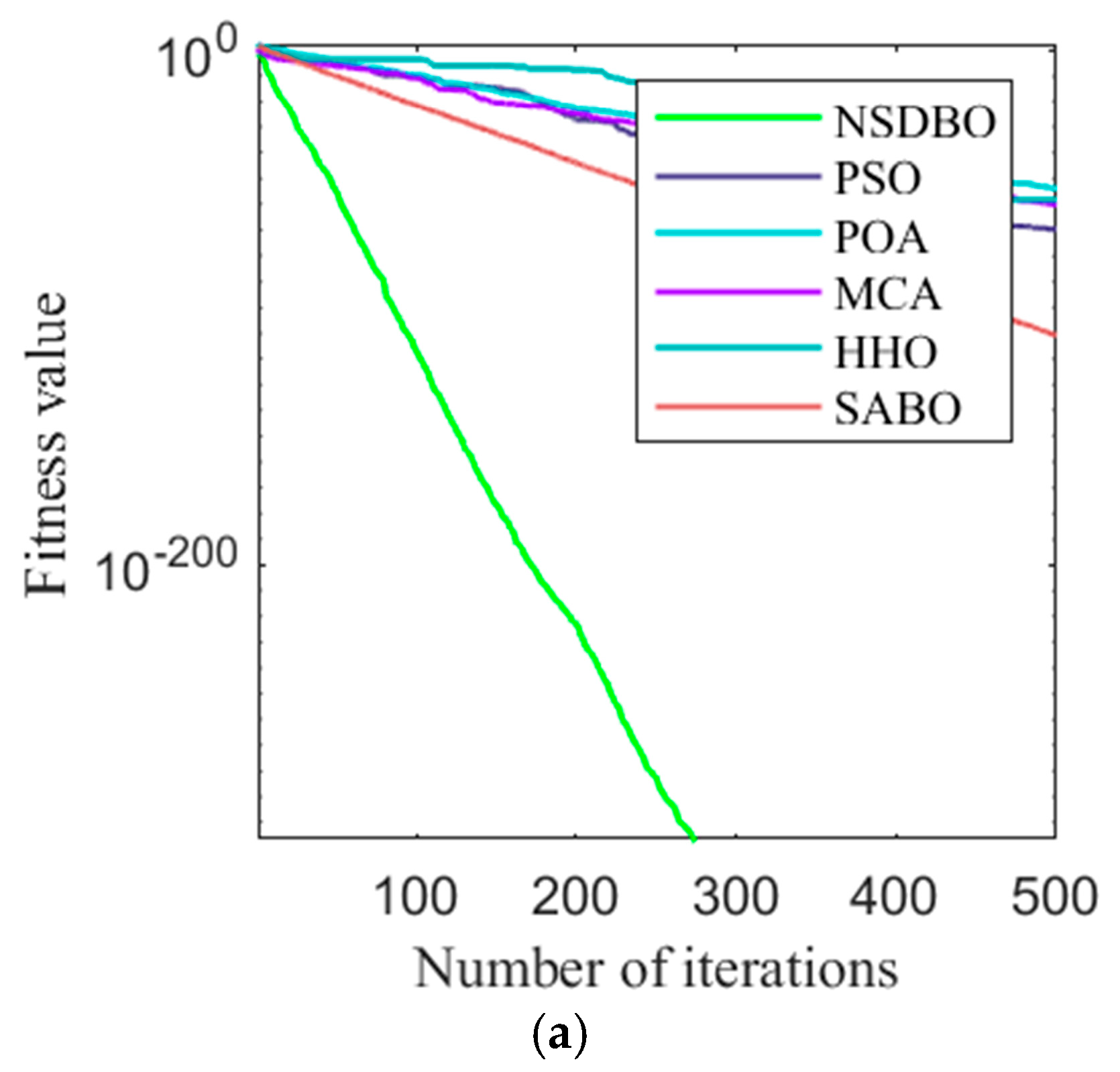
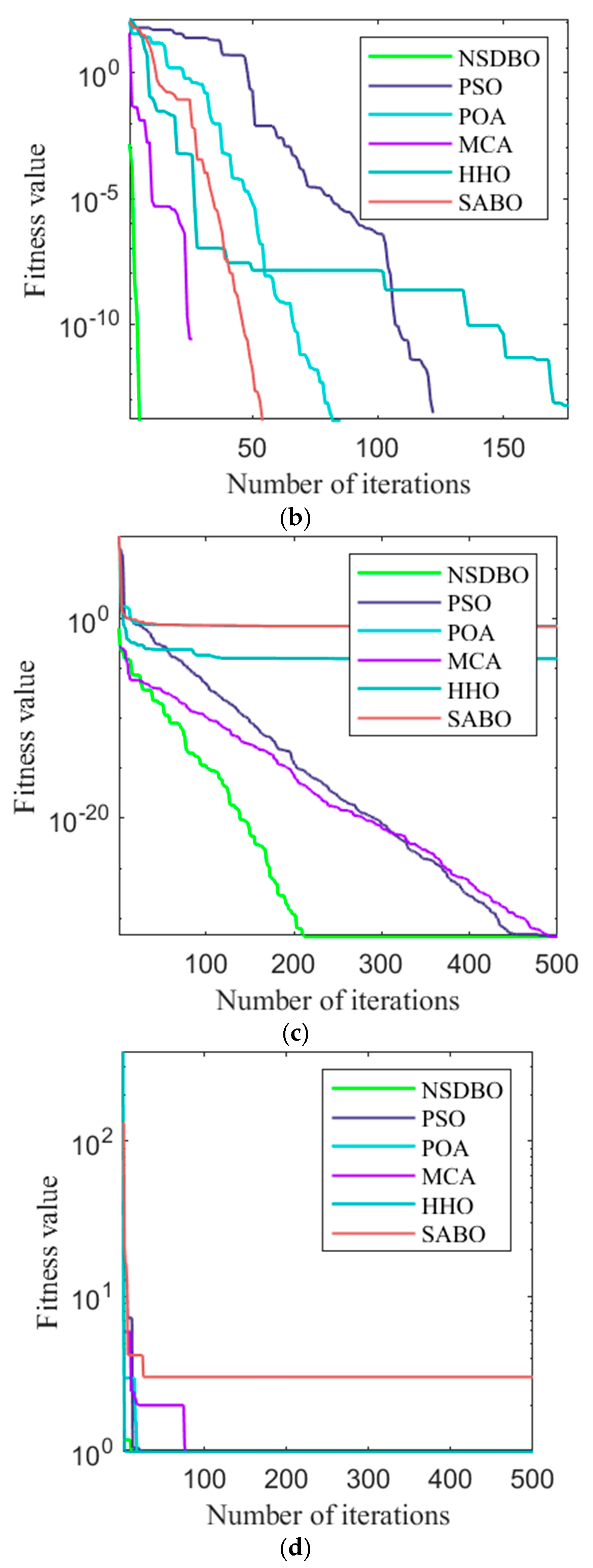
2.4.2. Model Performance Test

The NSDBO was tested using the CEC 2005 benchmark function set and compared with several leading intelligent optimization algorithms, including the Particle Swarm Optimization (PSO) [22], Musical Chairs Algorithm (MCA) [23], Pelican Optimization Algorithm (POA) [24], Subtraction-Average-Based Optimizer (SABO) [25], and Harris Hawk Optimization (HHO) [26]. The stability of the SBOA was evaluated using four representative test functions, with an initial population size of 40 and 500 iterations for each algorithm. The test function is shown in Appendix A 

Table A1. Test function set.

Benchmarking Functions	Search Space
$f_1={\displaystyle {\displaystyle \sum }_{i=1}^n}\left|x_i\right|+{\displaystyle {\displaystyle \prod }_{i=1}^n}\left|x_i\right|$	[−10, 10]
$f_2={\displaystyle {\displaystyle \sum }_{i=1}^n}\left[x_i^2-10\cos \left(2\pi x_i\right)+10\right]$	[−5.12, 5.12]
$\begin{array}{l}{f}_3=0.1\left\{si{n}^2\left(3\pi x_i\right)+{\left(x_i-1\right)}^2+{\displaystyle {\displaystyle \sum }_{i=1}^n}{\left(x_i-1\right)}^2\left[1+si{n}^2\left(3\pi x_i+1\right)\right]+\left[1+si{n}^2\left(2\pi x_i\right)\right]\right\}\\ +{\displaystyle {\displaystyle \sum }_{i=1}^n}u\left(x_i,5,100,4\right)\end{array}$	[−50, 50]
$f_4={\left[{\displaystyle \frac{1}{500}}+{\displaystyle {\displaystyle \sum }_{j=1}^{25}}{\displaystyle \frac{1}{j+{{\displaystyle \sum }}_{i=1}^2{\left(x_i-a_{ij}\right)}^6}}\right]}^{-1}$	[−65, 65]

, and the function convergence curve is shown in Appendix A Figure A1.

According to the results presented in Figure A1, the NSDBO demonstrated superior performance in terms of both optimal solution search and convergence speed compared to other algorithms. For the test functions ${\mathrm{f}}_1$, ${\mathrm{f}}_2$, and ${\mathrm{f}}_4$, NSDBO exhibited a notably faster convergence characteristic relative to the other algorithms. Furthermore, in ${\mathrm{f}}_3$, SBOA effectively addressed the local optimality issues often encountered by the traditional PSO and other algorithms, surpassing their capabilities in terms of optimal solution identification.

3. Results and Discussion

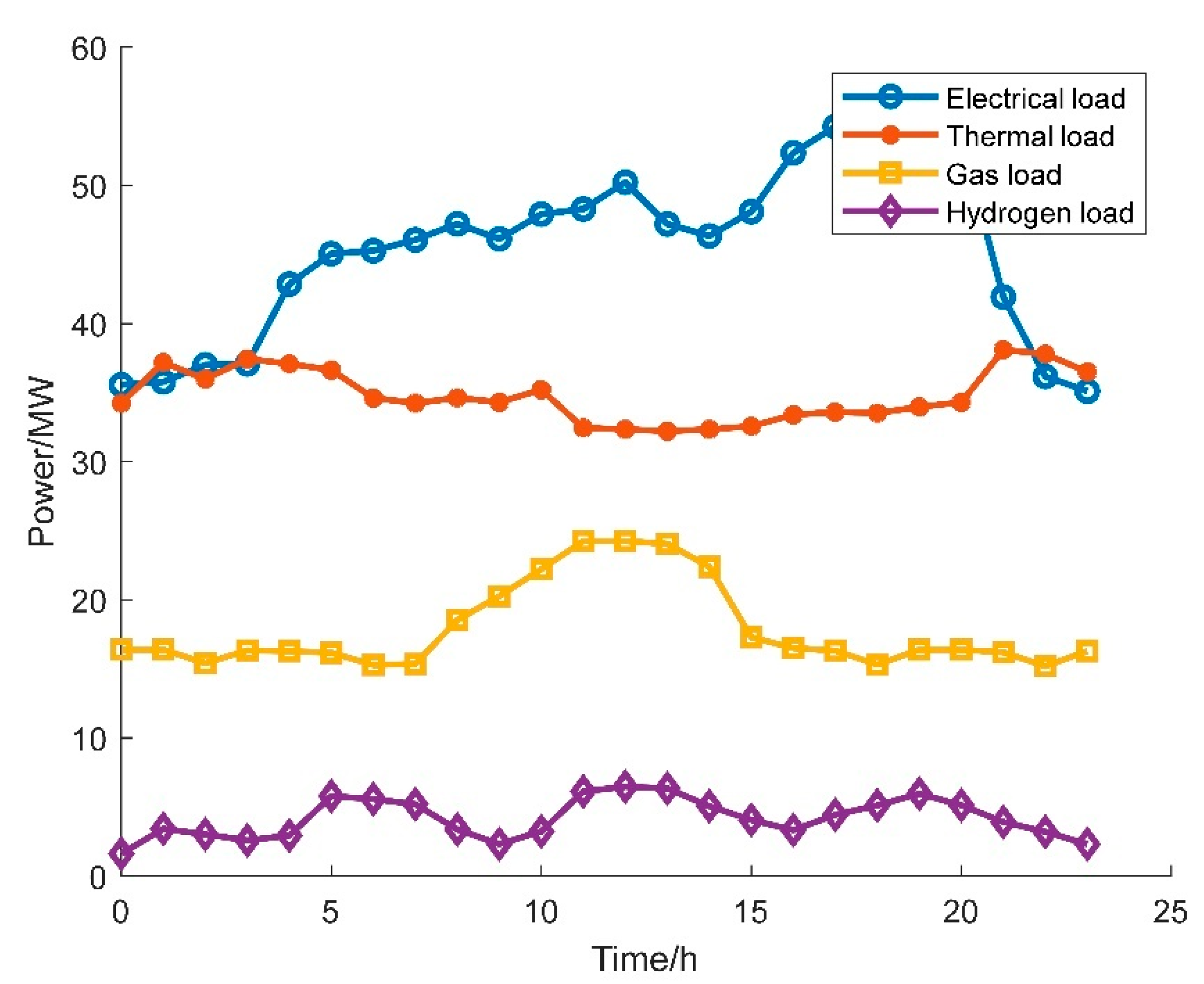
3.1. Basic Data

This study examines a comprehensive demonstration park in Northern China to analyze the percentage of wind and solar renewable energy across various scheduling scenarios, as well as to evaluate carbon dioxide emissions, carbon emission costs, and total operating costs. The scheduling period is established at 24 h with hourly time steps. Figure 5 illustrates the raw data for the electric, thermal, gas, and cooling load curves within the PIES framework. Electricity and natural gas prices vary over time, as referenced in literature [27].

Table 1. Parameters and economic parameters of each energy equipment in an industrial park.

Parameter	Numerical Value	Parameter	Numerical Value
$\alpha$	0.75	$c_{v2}$	−0.4
$\chi$	0.85	$\beta$	0.88
$P_{c,max}$(MW)	100	$T_{i,on,min}\left(h\right)$	6
$P_{c,min}$(MW)	0	$T_{i,off,min}\left(h\right)$	6
$P_{c2,max}$(MW)	30	$P_{i,max}$(MW)	100(NS), 100(MT), 25(RR)
$P_{c2,min}$(MW)	0	$P_{i,min}$(MW)	0(NS), 0(MT), 0(RR)
$P_{c0}^h$(MW)	50	$R_{i,up}$(MW)	10(CHP), 10(MT), 2.5(RR)
$c_{v1}$	−0.3	$R_{i,down}$(MW)	0(CHP), 0(MT), 0(RR)
$c_m$	1	${\eta }_{i,j}$	0.285(G2P,MT), 0.38(G2H,MT), 0.285(G2C,MT), 0.97(E2C,RR)
$\alpha$	0.75	$c_{v2}$	−0.4
$\chi$	0.85	$\beta$	0.88
$P_{c,max}$(MW)	100	$T_{i,on,min}\left(h\right)$	6
$P_{c,min}$(MW)	0	$T_{i,off,min}\left(h\right)$	6

presents the parameters and economic characteristics of the different energy devices within PIES. In Table 1, G2P refers to the conversion of natural gas to electricity, G2H to natural gas converted into thermal energy, G2C to natural gas converted into cooling energy, and E2C to electricity transformed into cooling energy. The allocation of carbon emissions rights for electricity, heat, and natural gas varies due to differences in their energy characteristics, market structures, technological innovations, and social acceptance. The electricity sector, with its diverse generation methods, requires more refined management, whereas the distribution of heat and natural gas focuses more on direct emissions control and the impacts over their entire lifecycle. According to the general knowledge of carbon emission right allocation in the China National Energy Administration and existing literature, this paper sets the free carbon emission right quota corresponding to per unit of electricity generation as 0.728 kg/(kWh), the free carbon emission right quota corresponding to per unit of heat generation as 0.385 kg/(kWh), and the free carbon emission right quota corresponding to per unit of gas load consumption as 0.180 kg/(kWh). The conversion coefficient from gas turbine power generation to heat, ${\sigma }_{e,h}$, is set at 0.75. The base price c for carbon trading is established at 0.034 USD/kg, with a trading volume range l of 4000 kg. The reward and punishment coefficients were set to 0.2 and 0.15, respectively, and the specific method reference is [28].

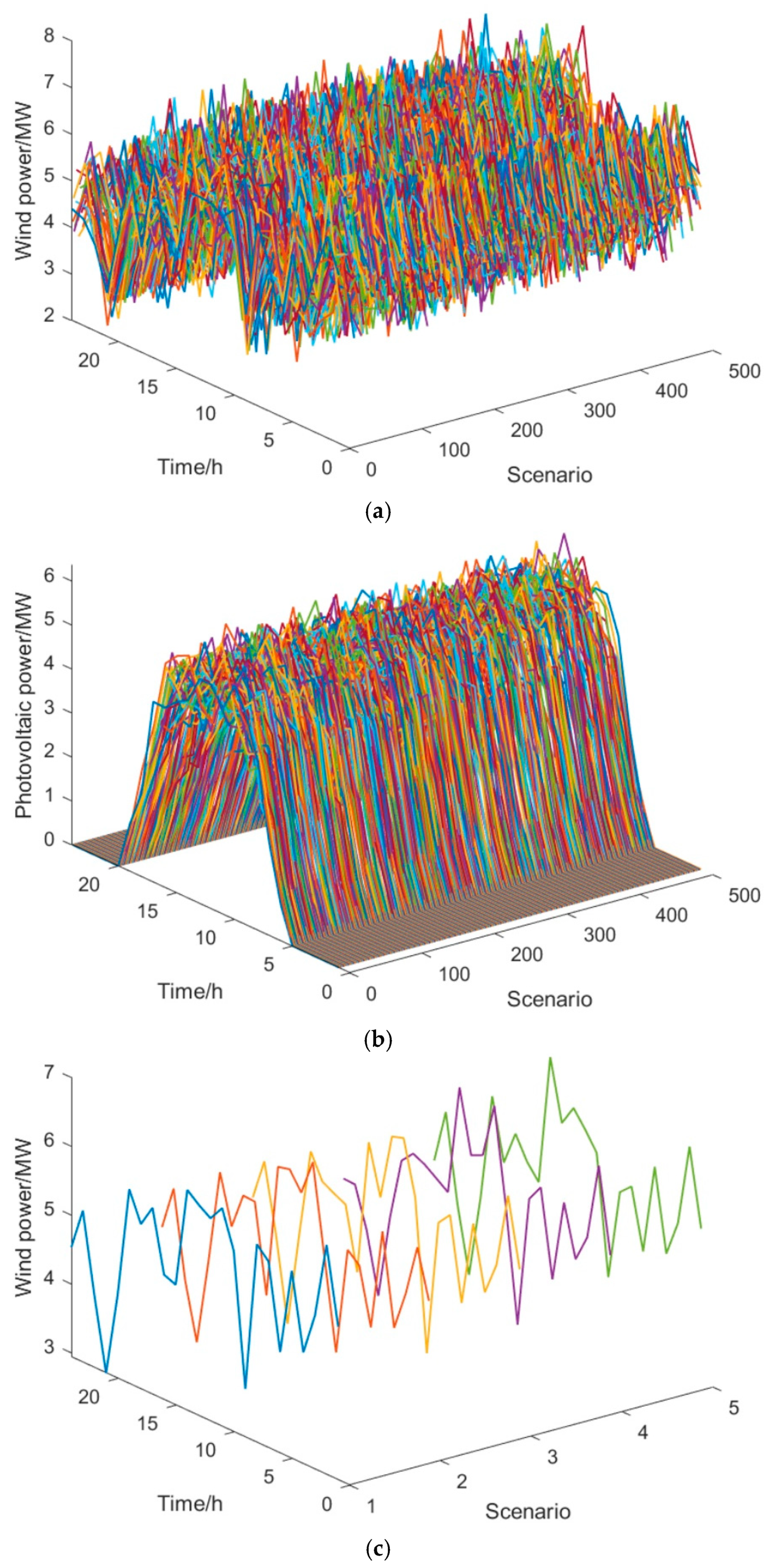
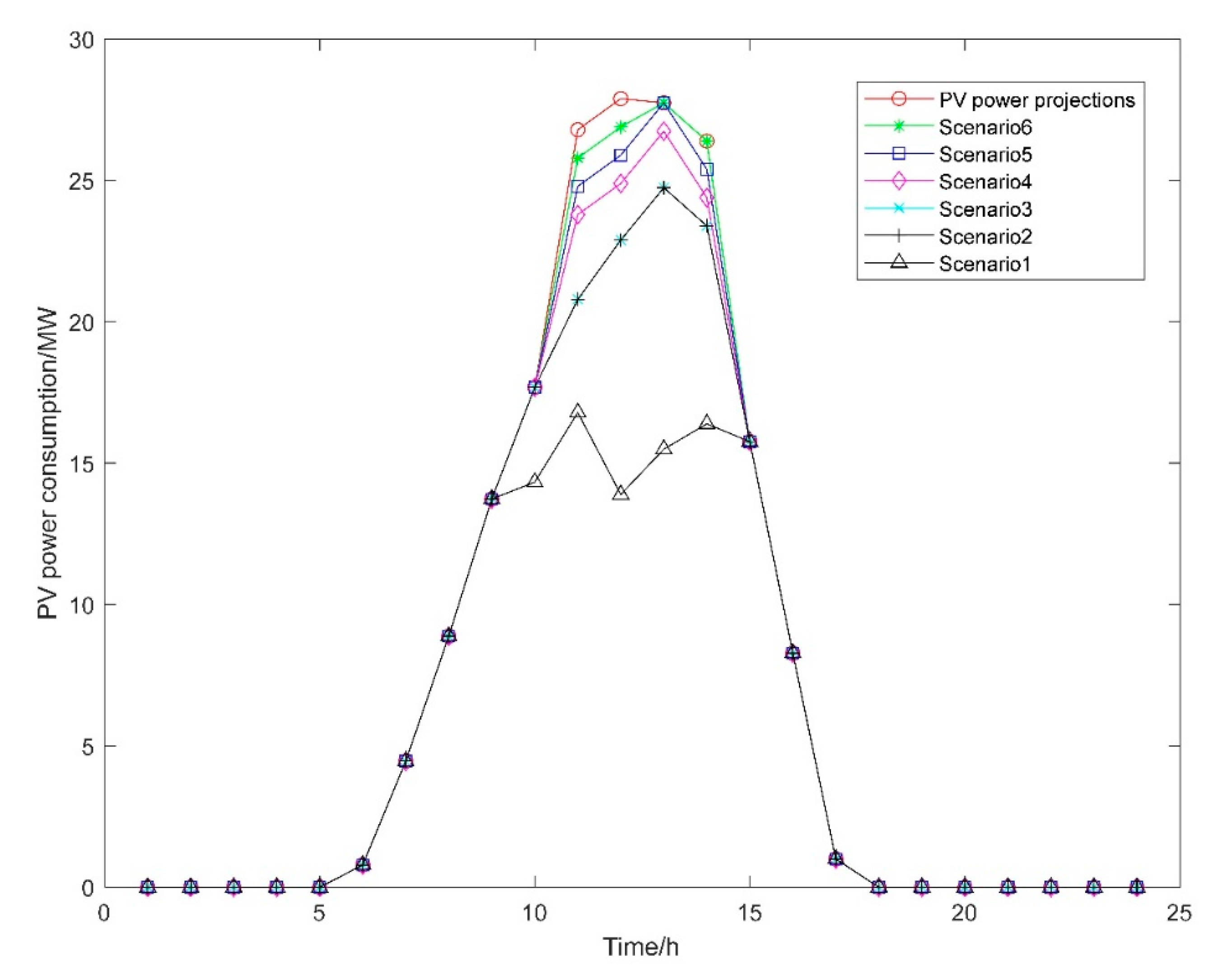
3.2. Generation and Reduction of Scenarios Considering Wind and Solar Uncertainty and Correlation

This section examines the uncertainties linked to wind and solar energy by utilizing forecasting data from the prior day, as detailed in Section 2. The findings are illustrated in Figure 6. Initially, we create 500 scenarios for wind and solar power output through a scenario generation technique that employs kernel density estimation and Copula theory. After that, we use the backward reduction method to refine the scene and finally select five representative scenarios for wind and solar power generation. The specific principles and proofs are detailed in [29]. The correlation probabilities of each scenario under the 95% confidence interval are listed in

Table 2. Probabilities corresponding to each scenario.

Scene	Probit
1	0.226
2	0.228
3	0.234
4	0.13
5	0.182

.

This approach integrates five representative scenarios of wind and solar output into the system’s optimal operational scheduling model, enabling the calculation of operational costs across various scenarios. Next, the operating costs for these five scenarios are combined probabilistically to establish the system’s final operational cost. This final value serves as an economic metric within the optimization scheduling model, leading to a scheduling strategy that effectively considers the uncertainties and correlations in wind and solar output.

3.3. Analysis of Optimization Scheduling Results

The NSDBO algorithm was utilized to solve the optimization scheduling problem, yielding a Pareto front solution set comprising 115 non-dominated solutions after several iterations. To further analyze the practical implications of the non-dominated solution values for engineering applications, we discuss the four solution methods under two objective functions in the context of various realistic trade-off scenarios that may arise. The scheduling results of the four methods under the 95% confidence interval are shown in

Table 3. Results of each method.

Operating Result	Methods 1	Methods 2	Methods 3	Methods 4
Operating costs/USD	11,633.65	33,338.64	19,207.90	22,797.95
Carbon emissions/kg	56,177.74	1238.71	11,438.22	9106.63
Environmental protection costs/USD	17,389.77	1486.79	3914.68	3426.38
Total cost/USD	29,023.41	34,825.43	23,122.59	26,224.33

. In this context, the compromise solution referenced in Method 4 refers to the use of a weighted scoring method that assigns equal weight factors to Methods 1–3 in the search for the optimal solution. These principles find their theoretical foundation in reference [30], which elaborates on a multi-objective optimization weighted scoring principle. In particular, it underscores the importance of assigning equal weight factors to competing objectives to ensure balanced overall solutions, providing crucial theoretical underpinnings for our selected approach. Furthermore, reference [30] highlights successful applications of this principle within specific engineering contexts, validating the practical feasibility of our optimization strategy.

Method 1: Finding the solution that minimizes operational costs.

Method 2: Finding the solution that minimizes environmental protection costs.

Method 3: Finding the solution that minimizes total costs.

Method 4: Normalizing and summing the values of the two objective functions, then selecting the particle corresponding to the minimum aggregated value, which identifies the compromise solution.

From Table 3, it can be concluded that there is no optimal scenario in which total costs, operational costs, and environmental protection costs can simultaneously be minimized. If the primary objective of the decision-maker is to achieve the lowest operational costs, then Method 1 should be employed for scheduling; under this approach, the operational costs are reduced by $21,704.99, $7574.26, and $11,164.30 compared to Methods 2, 3, and 4, respectively. If the decision-maker’s primary aim is to minimize environmental protection costs, then Method 2 should be selected, resulting in savings of $15,902.98, $2427.89, and $1939.59 in environmental protection costs relative to Methods 1, 3, and 4, respectively. Conversely, if the decision-maker seeks to minimize total costs, Method 3 should be utilized; in this case, the total costs saved would be $5900.82, $11,702.84, and $3101.74 compared to Methods 1, 2, and 4, respectively. Lastly, if the decision-maker aims to balance cost-effectiveness with low carbon emissions in search of a compromise solution, then Method 4 should be employed for scheduling.

3.3.1. Analysis of the Impact of Wind and Solar Output Uncertainty, Reward-Punishment Tiered Carbon Trading Mechanism, and Coupling Operation of P2G-CCS-CHP

This section explores the effects of considering the uncertainties in wind and solar outputs, a reward-punishment-tiered carbon trading mechanism, and the integrated operations of P2G, CCS, and CHP on the optimization results of PIES. Method 3, which prioritizes the minimization of total costs—a preferred solution approach for many decision-makers—is utilized for this analysis. Six distinct operational scenarios are established to assess the effectiveness of the scheduling strategy developed in this study. The optimization results of these scenarios under the 95% confidence interval are summarized in

Table 4. Optimized scheduling results for 6 scenarios.

Scenario	Operating Costs/USD	Environmental Protection Costs/USD	Total Cost/USD	Carbon Emissions/kg	WT Utilization Rate/%	PV Utilization Rate/%
Scenario 1	26,637.65	10,010.43	36,648.07	51177.74	53.44	65.27
Scenario 2	24,158.65	9122.30	33,280.95	47018.92	58.82	69.36
Scenario 3	22,005.03	7085.39	29,090.43	30645.65	60.62	70.10
Scenario 4	20,636.10	5445.35	26,081.45	19780.99	71.74	72.01
Scenario 5	19,805.39	4197.62	24,003.01	13589.00	77.90	80.21
Scenario 6	19,207.90	3914.68	23,122.59	11438.22	82.30	85.12

, while Figure 7, Figure 8 and Figure 9 depict the operational performance of the CHP unit’s power output, along with the absorption of wind and PV energy during the scheduling process. All scenarios and solutions are derived from the application of Method 3:

Scenario 1: Includes CHP but omits P2G, CCS, carbon trading mechanisms, and uncertainties related to wind and solar energy.

Scenario 2: Incorporates P2G-CHP while excluding CCS, carbon trading mechanisms, and wind and solar uncertainties.

Scenario 3: Considering the joint operation of P2G-CCS but the independent operation of the CHP system and the traditional carbon trading mechanism, the uncertainty of the scenery is not considered.

Scenario 4: Considering the P2G-CCS-CHP and the traditional step-by-step carbon trading mechanism, the uncertainty of scenery is not considered.

Scenario 5: Includes P2G-CCS-CHP with a reward-punishment-tiered carbon trading mechanism, excluding wind and solar uncertainties.

Scenario 6: Considers P2G-CCS-CHP, a reward-punishment-tiered carbon trading mechanism, and incorporates uncertainties related to wind and solar outputs (the model developed in this study).

Figure 7 illustrates that the comparison between Scenario 2 and Scenario 1 shows a reduction in grid-connected power output from the CHP unit during times of high renewable energy generation. This indicates that the P2G system is redirecting electrical power from the CHP unit. Additionally, the analysis of Scenario 3 compared to Scenario 2 reveals that when wind energy constitutes a significant portion of the energy supply, the grid power output from the CHP unit decreases further. This implies that the CCS system is utilizing CHP power to capture CO₂, thus lowering the net output of the CHP unit. In instances of elevated photovoltaic energy generation, the CHP unit does not contribute to the grid, as the thermal load demand is low and its generation capacity is minimal, resulting in the full conversion of its output into natural gas via the P2G system. When examining Scenarios 3, 4, and 5, it becomes evident that the carbon trading mechanisms do not significantly affect the power output of the CHP unit. Furthermore, when comparing Scenario 6 with Scenarios 4 and 5, the introduction of wind and solar output uncertainty leads to a decline in the hourly power output of the CHP within the PIES throughout the day, particularly pronounced during high renewable energy generation periods. This indicates that a detailed examination of the fluctuations and correlations in wind and solar output can improve the predictions of the daily wind-solar load curve. By optimizing the multi-energy coupling within the PIES and enhancing equipment flexibility, it is feasible to boost the integration of wind and solar energy while also minimizing the CHP unit’s power output.

Figure 8 illustrates critical time periods when wind power plays a substantial role in the energy supply, particularly between 00:00 and 05:00 and from 22:00 to 24:00. A comparison between Scenario 2 and Scenario 1 shows that integrating P2G into the CHP configuration enhances wind power absorption. This enhancement is mainly attributed to the P2G system’s capability to convert electricity into natural gas, thus creating extra storage for wind energy. In addition, examining Scenario 3 against Scenario 2 indicates that the CCS system provides CO₂ for the P2G process, reducing the need to source carbon externally. This results in lower operational costs for P2G, indicating that the inclusion of the P2G-CCS unit within the CHP structure boosts wind power absorption while cutting expenses. Comparing Scenario 4 to Scenario 3 reveals that the implementation of a tiered carbon trading system improves wind power absorption during high supply periods compared to scenarios lacking such mechanisms. This system increases the costs associated with managing carbon emissions, encouraging the PIES to absorb more wind energy to avoid excessive emissions. Moreover, the analysis of Scenario 5 in relation to Scenario 4 demonstrates that the penalty-reward carbon trading system is more effective than the traditional version. The enhanced penalties associated with stricter emission limits outweigh the additional costs incurred from higher wind power usage, leading to greater absorption. Lastly, evaluating Scenario 6 with respect to Scenario 5 shows that accounting for uncertainties in wind and solar outputs significantly increases the accuracy of daily wind power generation forecasts. This improvement ultimately supports the increasing wind power integration within the PIES framework.

Figure 9 shows that combining CHP and P2G in Scenario 2 significantly enhances the capacity to absorb PV power compared to Scenario 1. The P2G system effectively harnesses electricity, which increases the potential for integrating PV energy. In comparing Scenario 3 with Scenario 2, it becomes clear that CCS does not affect the absorption of PV power. Between 10:00 and 14:00, the output from CHP decreases due to lower heating demand and increased cooling demand. Consequently, under the constraints of CHP output, which includes P2G and CCS units, CCS fails to facilitate P2G conversion or improve PV electricity absorption. When analyzing Scenario 4 relative to Scenario 3, it is apparent that a tiered carbon trading system enhances PV power absorption during periods of high PV output compared to scenarios without it. This system raises carbon management costs, encouraging the PIES to consume more PV energy to reduce excess emissions. Additionally, the comparison of Scenario 5 with Scenario 4 shows that the penalty-reward tiered carbon trading system is more effective than the traditional model. The penalties imposed by stricter carbon emission limits outweigh the additional costs associated with increased PV usage, leading to higher absorption levels. Finally, the evaluation of Scenario 6 against Scenario 5 indicates that addressing the uncertainties associated with wind and solar generation significantly improves the accuracy of daily PV production forecasts. This enhancement is vital for optimizing PV absorption within the PIES framework.

An overview of Scenarios 1 to 6 presented in Table 4 illustrates that as the operational capacity of the PIES expands, the benefits of multi-energy complementarity and flexibility become increasingly evident, resulting in a steady reduction in operational costs. In particular, the comparison between scenario 4 and scenario 3 shows that the total cost and carbon emissions of the P2G-CCS-CHP joint operation are significantly lower than those of the three separate operations, and the utilization rate of new energy is significantly improved. The joint operation mechanism has advantages in scheduling. Furthermore, the collaboration of CHP and P2G improves energy conversion efficiency, minimizing energy losses and emissions. CCS technology captures CO₂ emissions, thus limiting their release into the atmosphere while supplying energy to P2G and decreasing reliance on external energy sources. The penalty-reward-tiered carbon trading system enhances the traditional approach by tightening carbon emission regulations and increasing penalties for exceeding limits. By incorporating the uncertainties of wind and solar energy, absorption rates for both types of energy are improved, fostering greater use of clean energy and contributing to a decrease in carbon emissions and environmental protection costs. Consequently, the simultaneous reduction in operational costs and environmental protection expenses optimizes total costs. Additionally, the effective scheduling of the PIES is dependent on the strategic allocation of wind and solar generation, which continues to boost the utilization of these renewable sources in scenarios characterized by multi-energy complementarity. The above improvement of energy saving and low carbon further proves the effectiveness of the strategy proposed in this paper.

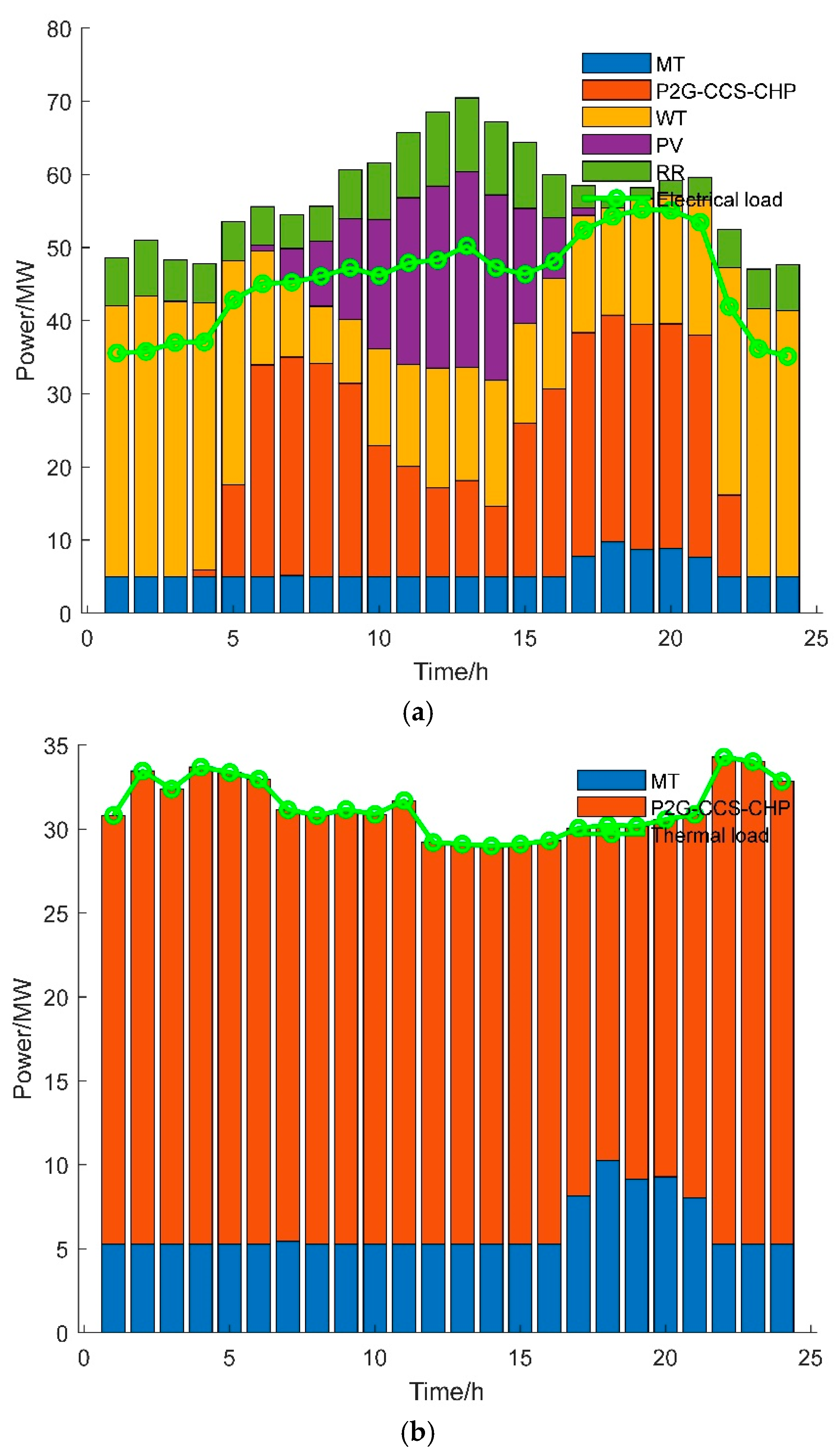
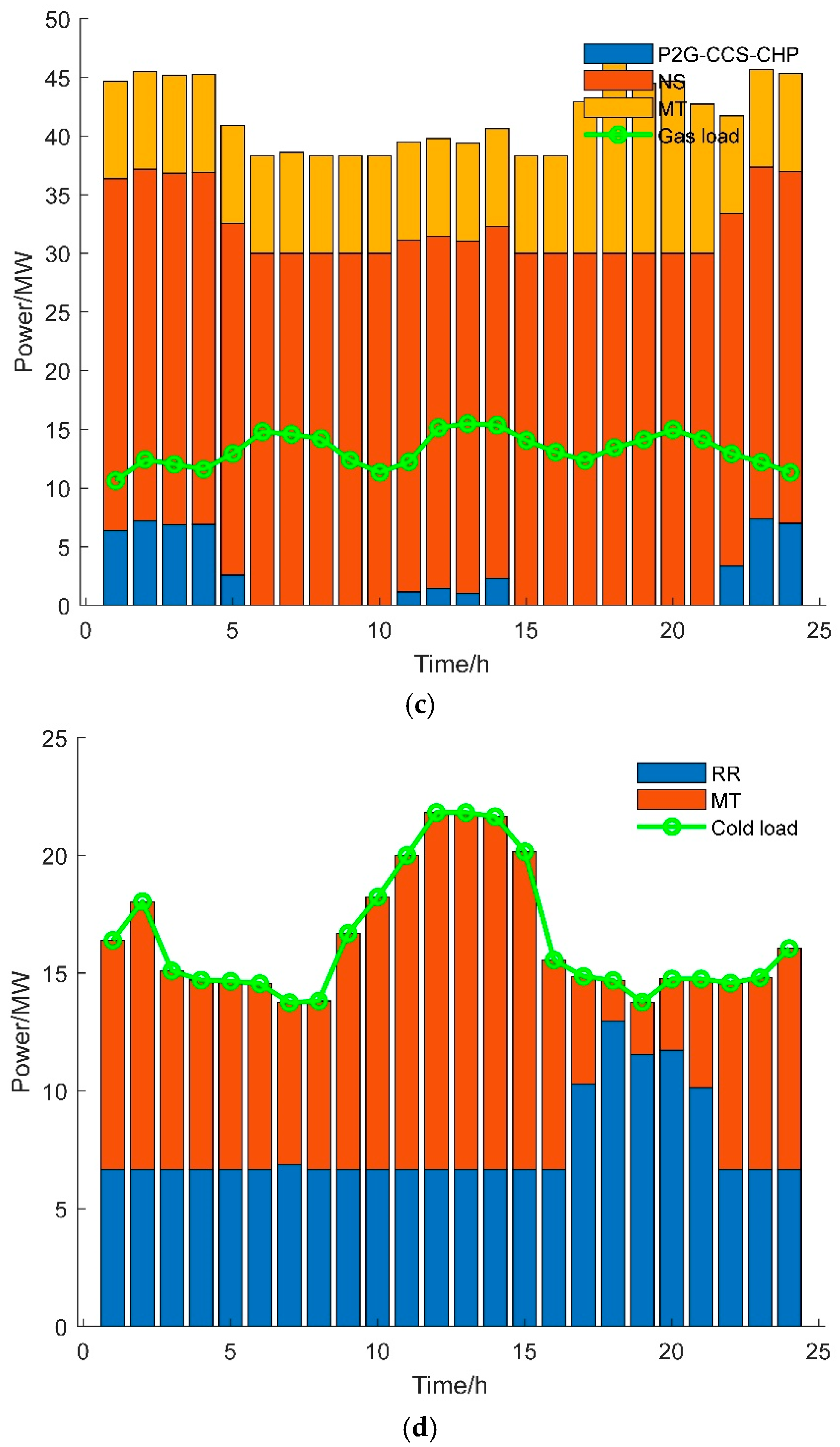
3.3.2. Analysis of PIES Optimal Scheduling in Scenario 6 (This Study’s Model)

The results from the optimal scheduling model developed in this study are presented in Figure 10 and Figure 11. The next section offers a comprehensive analysis to highlight its effectiveness and provide valuable insights for practical engineering applications.

Figure 10 depicts the performance of electrical, thermal, gas, and cooling power across each unit. In Figure 10a, the power generation unit meets the electrical load demand at all time intervals, with the P2G-CCS-CHP unit, WT, PV, and MT fulfilling both electricity and cooling needs. Figure 10b shows that the thermal load is delivered by the P2G-CCS-CHP unit in conjunction with the microturbines. Figure 10c reveals that the gas power utilized by the microturbines is sourced from both the gas supply and the P2G-CCS-CHP unit. Lastly, Figure 10d indicates that the cooling load is managed by the ER system and the microturbines.

Between the hours of 00:00–05:00, 10:00–15:00, and 22:00–24:00, when renewable energy generation is notably higher than during other times, the CHP system’s electrical output declines, shifting its focus to thermal energy, as shown in Figure 10a,b. Concurrently, the P2G system plays a significant role in gas energy production, as evidenced by Figure 10c. The CHP units face a “heat-determined-electricity” constraint that limits their capacity to utilize renewable energy effectively. Thus, the integration of P2G and CCS with the CHP system enables the conversion of electrical energy into gas energy, helping to ease the strong coupling constraints between electricity and heat in the CHP units. This synergy ultimately boosts the ability to absorb renewable energy. Additionally, refrigerators consume electrical energy to produce cooling energy, which partially satisfies the cooling load demand. This process alleviates the cooling load pressure on the microturbines, further reducing their electrical output and enhancing renewable energy integration.

During times of low renewable energy generation, CHP systems deliver considerable amounts of both electrical and thermal energy, as illustrated in Figure 10a,b. At these moments, the demand for thermal and electrical loads is relatively high, resulting in increased electrical output from the CHP units. In Figure 10c, the P2G system does not convert electrical energy into natural gas because renewable energy output is low and electrical power demand is high. To balance supply and demand, the P2G system avoids using the electrical energy produced by the CHP. Simultaneously, strategies such as using refrigerators to continuously consume electrical energy for cooling needs, increasing MT power output, enhancing the overall electrical output of the PIES, and reducing overall load demands are implemented to ensure reliable power supply.

When renewable energy generation is high and thermal load demands rise, the traditional “heat-led electricity” mode of CHP systems significantly limits the integration of renewable sources. In the research model, the CHP equipped with P2G and CCS units yields less electrical power but more thermal and gas power during high renewable generation periods. Conversely, in other timeframes, it produces less gas power while supplying more thermal and electrical energy, reflecting the interconnected nature of the three types of outputs. During periods of high renewable energy output, the P2G system captures the electrical energy generated by the CHP and converts it into gas energy, thus improving the capacity to harness renewable energy. The combined operation of the P2G-CCS-CHP system allows P2G and CCS to diminish the strong coupling between electrical and thermal outputs in CHP units, facilitating the transformation of electrical energy into gas energy to satisfy gas load requirements.

In the specific time frames of 00:00–05:00, 10:00–15:00, and 22:00–24:00, the CHP system integrated with P2G and CCS units effectively converts electrical energy into gas energy, thereby minimizing gas source output. This conversion results in reduced consumption of natural gas, leading to lower operating costs, decreased carbon emissions for the PIES, and reduced environmental protection expenses, as demonstrated in Figure 10c.

As illustrated in Figure 11, during the peak renewable energy generation times of 00:00–05:00, 10:00–15:00, and 22:00–24:00, P2G utilizes a significant amount of electricity produced by the CHP system, which encourages greater use of renewable energy to maintain a stable power supply. P2G requires CO₂ to consume electricity, and the CCS equipment captures the CO₂ emitted by the CHP system, supplying it to P2G. This setup alleviates the financial burden of obtaining carbon for P2G while also lowering the CHP’s carbon emissions. Consequently, the P2G-CCS-CHP system effectively reduces CO₂ emissions, environmental protection expenses, and operational costs while improving the integration capacity for renewable energy.

3.3.3. Analysis of the Impact of Reward and Penalty Coefficients on PIES Dispatching

As stated earlier, the tiered carbon trading mechanism based on rewards and penalties assesses actual carbon emissions against the initial carbon allowance. If emissions fall below this threshold, a subsidy is granted according to the reward coefficient; conversely, if they exceed the threshold, a penalty is imposed based on the penalty coefficient. Therefore, changes in the reward and penalty coefficients will directly impact the expenses related to carbon trading, in turn affecting the optimized operation of the PIES.

Figure 12 illustrates how varying values of the reward coefficient μ and penalty coefficient λ influence carbon trading costs for PIES. When carbon trading costs are positive, the penalty coefficient is applicable; in contrast, negative carbon trading costs indicate the activation of the reward coefficient.

The examination of Figure 12 yields several important insights:

(1)

In scenarios where carbon trading costs are negative, increasing the reward coefficient significantly amplifies the benefits that PIES gains from carbon trading. As carbon trading prices rise, these benefits progressively increase. This effect occurs because higher carbon trading revenues encourage PIES to minimize its dependence on external energy sources while boosting the efficiency of various energy supply and conversion devices within the system, ultimately leading to a significant reduction in overall carbon emissions.

(2)

In contrast, when carbon trading costs are positive, an increased penalty coefficient results in higher fines for PIES. To mitigate these penalties, PIES should strategically implement voluntary decarbonization scheduling. By integrating multi-energy coupling—encompassing electricity; heat; gas; and cooling—and employing energy conversion technologies such as Power-to-Gas (P2G); Carbon Capture and Storage (CCS); and Combined Heat and Power (CHP); these scheduling efforts can create situations where a higher penalty coefficient corresponds with lower carbon trading costs.

(3)

During PIES’s operational scheduling, it is critical to manage the interplay between reward and penalty coefficients and carbon trading costs to identify the optimal balance point. Achieving this balance is essential for reducing carbon emissions while ensuring the economic viability of scheduling practices. This could involve establishing distinct thresholds for reward and penalty adjustments based on real-time trading data and market trends.

(4)

Fluctuations in carbon trading prices will directly impact the associated revenues or costs for PIES. Therefore, it is vital to establish a dynamic strategy to adjust operational scheduling in response to these price changes, maximizing revenues or minimizing costs effectively in real-time.

(5)

PIES must enhance its monitoring and analysis of the carbon trading market to stay informed about market trends and price movements. Continuous monitoring will provide valuable data to inform scheduling decisions, enhancing responsiveness to market changes. Key focus areas include tracking emerging regulations, competitor behaviors, and shifts in overall market demand, allowing for better-informed adjustments to operational strategies.

4. Conclusions Implications and Future Research Orientations

This research focuses on optimizing the low-carbon operations of integrated energy systems in parks that utilize wind and solar energy alongside the multi-energy coupling of electricity, heat, gas, and cooling. We introduce a tiered reward-and-punishment carbon trading mechanism that accounts for the uncertainties and interrelationships in renewable energy output, as well as the integration of P2G, CCS, and CHP for the economically efficient low-carbon scheduling of PIES. The simulation analysis of practical scenarios leads to several findings:

(1)

The proposed reward-punishment tiered carbon trading mechanism achieves substantial decarbonization performance, reducing PIES carbon emissions by 31.30% (6191.99 kg) compared to conventional mechanisms. This regulatory innovation establishes critical financial incentives that align market dynamics with environmental objectives, providing a policy-relevant framework for low-carbon transition management.

(2)

Through probabilistic modeling of renewable energy uncertainties and inter-source correlations, our framework enhances system sustainability across three dimensions: economic efficiency (+3.67% cost reduction/$880.42 savings), environmental performance (15.83% emission reduction/2150.78 kg mitigation), and renewable utilization (4.4% wind and 4.91% solar consumption increases). This tripartite optimization addresses the energy trilemma challenges in integrated energy systems.

(3)

The novel P2G-CCS-CHP coupling model demonstrates paradigm-shifting improvements over conventional systems. Relative to traditional CHP configurations, it achieves 28.86% wind and 19.85% solar utilization enhancements alongside a remarkable 36.91% cost reduction and 77.65% emission abatement. When benchmarked against existing P2G-CCS integrations, the proposed architecture further improves renewable consumption (21.68% wind, 15.02% solar) while reducing costs and emissions by 20.51% and 62.68%, respectively. These comparative results validate the technical superiority of our multi-system coupling approach.

(4)

The biomimetic non-dominated sorting dung beetle optimizer introduces strategic multi-objective optimization capabilities, demonstrating 18–32% computational efficiency gains over PSO, MCA, POA, SABO, and HHO algorithms in Pareto front identification. This bio-inspired metaheuristic effectively resolves the convergence-precision trade-off in complex energy system optimizations.

While this study establishes methodological advancements in integrated energy system optimization, two critical methodological constraints warrant explicit discussion. First, the static treatment of carbon emission factors in our model overlooks the temporal and spatial variability inherent in practical emission accounting systems. This simplification may underestimate the operational adaptability required for real-time policy compliance, particularly in jurisdictions implementing dynamic carbon pricing mechanisms or region-specific emission coefficients. Second, the exclusion of voluntary emission reduction mechanisms—including carbon offset programs; renewable energy certificate trading; and corporate sustainability initiatives—constrains the model’s alignment with contemporary market-driven decarbonization practices. These omitted mechanisms constitute essential components of modern carbon management frameworks in most industrialized nations, potentially affecting the generalizability of our economic optimization results in policy-integrated scenarios.

To address these knowledge gaps, our future research agenda will pursue three strategic directions: (1) Developing adaptive carbon accounting modules that incorporate time-variant emission factors and cross-regional carbon flow tracking; (2) Integrating hybrid market mechanisms combining mandatory compliance systems with voluntary carbon market dynamics; (3) Implementing multi-temporal scale optimization considering both short-term operational flexibility (hourly resolution) and long-term infrastructure planning (decadal horizons). This expanded framework aims to bridge the current model’s theoretical assumptions with the complex system dynamics observed in emerging carbon-neutrality transition pathways.

References

1. Drosos, D.; Kyriakopoulos, G.L.; Arabatzis, G.; Tsotsolas, N. Evaluating Customer Satisfaction in Energy Markets Using a Multicriteria Method: The Case of Electricity Market in Greece. Sustainability 2020, 12, 3862. [Google Scholar] [CrossRef]
2. Shafiullah, M.; Ahmed, S.D.; Al-Sulaiman, F.A. Grid Integration Challenges and Solution Strategies for Solar PV Systems: A Review. IEEE Access 2022, 10, 52233–52257. [Google Scholar] [CrossRef]
3. Sinha, S.; Chandel, S.S. Review of recent trends in optimization techniques for solar photovoltaic-wind based hybrid energy systems. Renew. Sustain. Energy Rev. 2015, 50, 755–769. [Google Scholar] [CrossRef]
4. Zhao, G.; Wan, C.X.; Zuo, W.Q.; Zhang, K.F.; Shu, X.Y. Research on Multiobjective Optimal Operation Strategy for Wind-Photovoltaic-Hydro Complementary Power System. Int. J. Photoenergy 2022, 2022, 5209208. [Google Scholar] [CrossRef]
5. Ju, L.; Tan, Z.; Yuan, J.; Tan, Q.; Li, H.; Dong, F. A bi-level stochastic scheduling optimization model for a virtual power plant connected to a wind-photovoltaic-energy storage system considering the uncertainty and demand response. Appl. Energy 2016, 171, 184–199. [Google Scholar] [CrossRef]
6. Liu, X.H.; Li, X.; Tian, J.Q.; Wang, Y.B.; Xiao, G.X.; Wang, P. Day-Ahead Economic Dispatch of Renewable Energy System considering Wind and Photovoltaic Predicted Output. Int. Trans. Electr. Energy Syst. 2022, 2022, 6082642. [Google Scholar] [CrossRef]
7. Xu, M.; Cui, Y.; Wang, T.; Zhang, Y.Z.; Guo, Y.; Zhang, X.Y. Optimal Dispatch of Wind Power, Photovoltaic Power, Concentrating Solar Power, and Thermal Power in Case of Uncertain Output. Energies 2022, 15, 8215. [Google Scholar] [CrossRef]
8. Min, H.L.; He, P.K.; Li, C.L.; Yang, L.B.; Xiao, F. The Temporal and Spatial Characteristics of Wind-Photovoltaic-Hydro Hybrid Power Output Based on a Cloud Model and Copula Function. Energies 2024, 17, 1024. [Google Scholar] [CrossRef]
9. Chen, S.T.; Su, W.H.; Wu, B.Y. Two stage robust planning of park integrated energy system considering low carbon. Front. Ecol. Evol. 2023, 10, 1100089. [Google Scholar] [CrossRef]
10. Zhang, Y.L.; Zhang, P.H.; Du, S.; Dong, H.L. Economic Optimal Scheduling of Integrated Energy System Considering Wind-Solar Uncertainty and Power to Gas and Carbon Capture and Storage. Energies 2024, 17, 2770. [Google Scholar] [CrossRef]
11. Zhu, D.Y.; Cui, J.; Wang, S.J.; Wei, J.Z.; Li, C.R.; Zhang, X.M.; Li, Y.Z. An optimization strategy for intra-park integration trading considering energy storage and carbon emission constraints. J. Clean. Prod. 2024, 447, 141031. [Google Scholar] [CrossRef]
12. Liu, L.; Qin, Z.J. Low-carbon planning for park-level integrated energy system considering optimal construction time sequence and hydrogen energy facility. Energy Rep. 2023, 9, 554–566. [Google Scholar] [CrossRef]
13. Zhang, J.L.; Liu, Z.Y. Low carbon economic scheduling model for a park integrated energy system considering integrated demand response, ladder-type carbon trading and fine utilization of hydrogen. Energy 2024, 290, 130311. [Google Scholar] [CrossRef]
14. Li, K.; Ying, Y.L.; Yu, X.Y.; Li, J.C. Optimal Scheduling of Electricity and Carbon in Multi-Park Integrated Energy Systems. Energies 2024, 17, 2119. [Google Scholar] [CrossRef]
15. Chen, C.M.; Liu, C.; Ma, L.Y.; Chen, T.W.; Wei, Y.Q.; Qiu, W.Q.; Lin, Z.Z.; Li, Z.Y. Cooperative-game-based joint planning and cost allocation for multiple park-level integrated energy systems with shared energy storage*. J. Energy Storage 2023, 73, 108861. [Google Scholar] [CrossRef]
16. Chen, H.Y.; Wang, S.C.; Yu, Y.X.; Guo, Y.; Jin, L.; Jia, X.Q.; Liu, K.C.; Zhang, X.H. Low-Carbon Operation Strategy of Park-Level Integrated Energy System with Firefly Algorithm. Appl. Sci. 2024, 14, 5433. [Google Scholar] [CrossRef]
17. Wang, L.L.; Xian, R.C.; Jiao, P.H.; Liu, X.H.; Xing, Y.W.; Wang, W. Cooperative operation of industrial/commercial/residential integrated energy system with hydrogen energy based on Nash bargaining theory. Energy 2024, 288, 129868. [Google Scholar] [CrossRef]
18. Xu, F.Q.; Li, X.P.; Jin, C.H. A multi-objective operation optimization model for the electro-thermal integrated energy systems considering power to gas and multi-type demand response. J. Renew. Sustain. Energy 2024, 16, 045301. [Google Scholar] [CrossRef]
19. Ding, X.Y.; Yang, Z.P.; Zheng, X.B.; Zhang, H.; Sun, W. Effect of decision-making principle on P2G-CCS-CHP complementary energy system based on IGDT considering energy uncertainty. Int. J. Hydrogen Energy 2024, 81, 986–1002. [Google Scholar] [CrossRef]
20. Vachhani, V.L.; Dabhi, V.K.; Prajapati, H.B. Improving NSGA-II for solving multi objective function optimization problems. In Proceedings of the 2016 International Conference on Computer Communication and Informatics, Coimbatore, India, 7–9 January 2016; pp. 1–6. [Google Scholar]
21. Xue, J.; Shen, B. Dung beetle optimizer: A new meta-heuristic algorithm for global optimization. J. Supercomput. 2022, 79, 7305–7336. [Google Scholar] [CrossRef]
22. Kennedy, J.; Eberhart, R. Particle swarm optimization. In Proceedings of the ICNN’95—International Conference on Neural Networks, Perth, WA, Australia, 27 November–1 December 1995; Volume 4, pp. 1942–1948. [Google Scholar] [CrossRef]
23. Eltamaly, A.M.; Rabie, A.H. A Novel Musical Chairs Optimization Algorithm. Arab. J. Sci. Eng. 2023, 48, 10371–10403. [Google Scholar] [CrossRef]
24. Trojovsky, P.; Dehghani, M. Pelican Optimization Algorithm: A Novel Nature-Inspired Algorithm for Engineering Applications. Sensors 2022, 22, 855. [Google Scholar] [CrossRef] [PubMed]
25. Trojovsky, P.; Dehghani, M. Subtraction-Average-Based Optimizer: A New Swarm-Inspired Metaheuristic Algorithm for Solving Optimization Problems. Biomimetics 2023, 8, 149. [Google Scholar] [CrossRef] [PubMed]
26. Heidari, A.A.; Mirjalili, S.; Faris, H.; Aljarah, I.; Mafarja, M.; Chen, H.L. Harris hawks optimization: Algorithm and applications. Future Gener. Comput. Syst.-Int. J. Escience 2019, 97, 849–872. [Google Scholar] [CrossRef]
27. Li, Y.; Zou, Y.; Tan, Y.; Cao, Y.J.; Liu, X.D.; Shahidehpour, M.; Tian, S.M.; Bu, F.P. Optimal Stochastic Operation of Integrated Low-Carbon Electric Power, Natural Gas, and Heat Delivery System. IEEE Trans. Sustain. Energy 2018, 9, 273–283. [Google Scholar] [CrossRef]
28. Lu, Q.; Guo, Q.S.; Zeng, W. Optimization scheduling of an integrated energy service system in community under the carbon trading mechanism: A model with reward-penalty and user satisfaction. J. Clean. Prod. 2021, 323, 129171. [Google Scholar] [CrossRef]
29. Ba-swaimi, S.; Verayiah, R.; Ramachandaramurthy, V.K.; Alahmad, A.K. Long-term optimal planning of distributed generations and battery energy storage systems towards high integration of green energy considering uncertainty and demand response program. J. Energy Storage 2024, 100, 113562. [Google Scholar] [CrossRef]
30. Zhang, X.Z.; Wang, Z.Y.; Lu, Z.Y. Multi-objective load dispatch for microgrid with electric vehicles using modified gravitational search and particle swarm optimization algorithm. Appl. Energy 2022, 306, 118018. [Google Scholar] [CrossRef]
Figure 1. Integrated energy system framework of the park.
Processes 13 00680 g001
Figure 2. Electro-thermal coupling characteristics of CHP and P2G-CCS-CHP.
Processes 13 00680 g002
Figure 3. P2G-CCS-CHP multi-energy output relationship.
Processes 13 00680 g003
Figure 4. Flowchart of NSDBO algorithm.
Processes 13 00680 g004
Figure 5. Raw data of electrical, thermal, air, and cooling loads inside PIES.
Processes 13 00680 g005
Figure 6. Generation and reduction of landscape scene: (a) Generation of 500 Wind Power Output Scenarios Considering; (b) Generation of 500 Photovoltaic Output Scenarios Considering; (c) Five Scenarios of Wind Power Output After Reduction; (d) Five Scenarios of Photovoltaic Output After Reduction.
Processes 13 00680 g006aProcesses 13 00680 g006b
Figure 7. Comparison of CHP power for six scenarios.
Processes 13 00680 g007
Figure 8. Comparison of Wind Power Consumption in Six Scenarios.
Processes 13 00680 g008
Figure 9. Comparison of PV consumption in six scenarios.
Processes 13 00680 g009
Figure 10. Optimal scheduling results for PIES in scenario 6: (a) Power Balance Diagram of PIES in Scenario 6; (b) Thermal Power Balance Diagram of PIES in Scenario 6; (c) Gas Power Balance Diagram of PIES in Scenario 6; (d) Cold Power Balance Diagram of PIES in Scenario 6.
Processes 13 00680 g010aProcesses 13 00680 g010b
Figure 11. P2G power consumption vs. CO2 capture by CCS in Scenario 6.
Processes 13 00680 g011
Figure 12. Effect of incentive and penalty coefficients on PIES carbon trading costs.
Processes 13 00680 g012