Abstract
The independent metering system (IMS) realizes the independent adjustments of oil inlet and oil return by decoupling the control of the inlet and outlet orifices of the valve, which can significantly improve the energy utilization efficiency while ensuring the tracking accuracy of the system. In this paper, a predetermined performance control (PPC) strategy based on adaptive output feedback is proposed. Firstly, the K-filter observer is introduced into the IMS framework for the purpose of obtaining accurate estimates of the internal state variables that are not directly measurable. Secondly, the fuzzy logic system (FLS) is used to effectively compensate for the unmodeled error and external disturbance in system dynamics. Furthermore, by incorporating PPC, the control objective is to guarantee that all state errors converge to and remain within the prescribed performance function boundaries within a given time frame. At the same time, the dynamic surface control (DSC) method is used to alleviate the common ‘computational explosion’ problem in the backstepping design. In addition, the oil return pressure controller is designed to maintain the oil return back pressure at a low level, thereby reducing the pressure loss in the oil return path and improving the overall energy efficiency of the system. The theoretical analysis results show that the proposed controller can effectively improve the energy efficiency of the system while ensuring the tracking accuracy. Finally, the effectiveness and superiority of the control strategy are verified by comparative experiments.
1. Introduction
Due to its high power-to-weight ratio and power density, the hydraulic transmission system is widely used in various types of walking machinery and industrial equipment [1,2]. In the traditional hydraulic system, the multi-way valve used to control the actuator usually adopts the design of the mechanical coupling of inlet and outlet [3], which is difficult to adjust flexibly according to the actual working conditions, resulting in poor control accuracy of the actuator and significant energy loss of valve orifice throttling [4]. As a new type of fluid power control system, the independent metering system (IMS) can effectively alleviate the problem of high energy consumption. The system breaks through the adjustment mode of the linkage of the inlet and return valve ports in the traditional valve control. By independently controlling the opening of the inlet and return valve ports, the decoupling control of the pressure and flow of the two chambers of the actuator is realized, thus greatly improving the energy efficiency and operating performance of the system [5].
In the controller design, it is usually necessary to obtain the position, velocity and pressure signals of the system at the same time. However, in practical engineering applications, due to the limitations of cost and environmental factors, the measurement of speed and pressure is often accompanied by strong noise, resulting in it being difficult for the control strategy based on full state feedback to achieve ideal performance in practice, and even in performance degradation [6,7,8,9]. In order to solve this problem, a nonlinear position control strategy combining backstepping control and extended state observer is developed in [10], which ensures that the system states asymptotically converge to the desired values with both speed and stability. The simulation results show that the proposed method is superior to the traditional PI control in control performance. In addition, in order to effectively suppress the external disturbance and model uncertainty in the hydraulic system, references [11,12] proposed fusing the disturbance observer and the extended state observer to jointly estimate the total disturbance and unmodeled dynamics of the system, thus achieving high-precision tracking within a backstepping control framework for the electro-hydraulic servo valve system. The control structure has been verified on the experimental platform of the Moog servo double-rod actuator.
Unmodeled dynamics and external disturbances represent inherent challenges that complicate the design of controllers and may adversely affect the stability of closed-loop control systems [13,14,15]. Previous work on output feedback tracking for nonlinear time-delay systems has utilized adaptive neural networks to mitigate the effects of unknown nonlinearities [16,17]. Similarly, a fuzzy logic system (FLS) was applied in [18] to estimate uncertainties within the system and achieve high-precision tracking performance. In recent years, numerous studies have integrated neural networks or FLSs with adaptive control strategies to handle uncertainties in nonlinear functions, leading to extensive advances in this area [19,20]. The concept of prescribed performance control (PPC) was initially introduced by the Greek scholar G. Rovithakis et al. [21] and has since evolved into a widely adopted methodology for constraining state tracking errors in hydraulic systems. The core principle of PPC involves designing a prescribed performance function (PPF), typically an adjustable exponential decay function, to enforce the desired transient and steady-state performance [22,23,24]. As system variables (e.g., output signals or tracking errors) approach predefined bounds, the controller adjusts accordingly to prevent the violation of these constraints, thereby maintaining consistent performance specifications. To achieve accurate tracking under time-varying disturbances and parametric uncertainties while complying with preset performance criteria, PPC has been combined with adaptive control techniques. This integration has proven effective in attaining robust and precise tracking in hydraulic servo systems [25,26].
Another motivation of this study is that the existing control methods mainly focus on the actuator’s control accuracy improvement while ignoring the system energy efficiency. Using the independent metering hydraulic system [27,28], the decoupling control of the pressure of the two capacitive cavities can be realized by employing multiple spools to control the flow rate of the actuator inlet and outlet independently, thus reducing the oil supply pressure of the pump source and achieving a certain energy-saving effect [29,30,31]. Thus, the control system must not only handle the aforementioned nonlinear models and uncertainties, but also incorporate energy-saving characteristics while ensuring high accuracy to effectively improve the system’s energy efficiency.
The existing research pays limited attention to the realization of the predetermined tracking accuracy of the IMS. Especially in the case of only obtaining position signals and time-varying disturbances, how to ensure system stability and high-precision trajectory tracking at the same time is still an urgent problem to be solved. Inspired by related research, this paper is devoted to achieving high-precision tracking control of the IMS under the above conditions. The main contributions include the following three aspects:
- The K-filter theory is innovatively applied to the load port of the IMS, which realizes the accurate estimation of the unmeasurable state quantity in the system, provides the necessary state information for the subsequent control, and overcomes the dependence of the traditional full state feedback on the sensor.
- The FLS is used to adaptively compensate for the unmodeled dynamics and external disturbances of the system, and the PPC is introduced to ensure that all state errors are strictly constrained within the preset performance function boundary within the set time, which effectively improves the control accuracy and robustness of the system.
- The DSC method is used to simplify the backstepping design process and alleviate the ‘computational explosion’ problem. In addition, the oil return pressure controller is specially designed to actively maintain the oil return back pressure at a low level, which reduces the energy loss on the oil return path of the system, thus improving the energy utilization efficiency of the system as a whole.
The remainder of this paper is organized as follows. Section 2 presents the system modeling and necessary preliminaries. Following this, Section 3 details the design of the extended state observer. Subsequently, Section 4 provides the design and stability analysis for both the adaptive fuzzy tracking controller and the oil return pressure controller. In Section 5, the effectiveness of the proposed control algorithm is verified by experiments. Section 6 summarizes the work of this paper.
2. System Model Description and Preliminary Explanation
2.1. Kinetic Model of Hydraulic Systems
The typical structure of the load port’s independent hydraulic system is shown in Figure 1. The system consists of the proportional valve, hydraulic cylinder, inertial load, and position sensor.
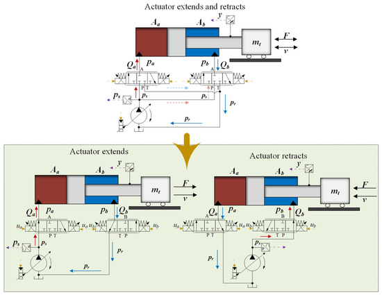
Figure 1.
Load port independent position feedback hydraulic control system.
The force balance equation of inertial load can be expressed as follows:
Here, and denote the pressures within the inlet and return oil chambers, respectively. Correspondingly, and are the effective piston areas of the cylinder’s large and small chambers. The variable represents the cylinder displacement. The term models the sliding friction force, while encapsulates all unknown disturbances in the dynamics, comprising unmodeled friction, damping effects, model uncertainties, and external disturbances.
The flow continuity equation for the hydraulic cylinder, which accounts for the compressibility of the hydraulic oil, is expressed as follows:
where , given that the bandwidth of the proportional valve significantly exceeds that of the overall system, is the effective bulk modulus of the hydraulic oil, is the control volume of the respective cylinder chamber (either chamber A or B), simplified to the proportional link, , and is the gain. Therefore,
In the formula, , and
where Qa, Qb are the flow rates into chambers A and B, respectively, and g is a total gain coefficient. Kq is the flow gain coefficient. Ki is the gain of the proportional valve. Cd is the discharge coefficient. W is the area gradient of the valve orifice. ua, ub are the independent control signals for Valve A and Valve B, respectively. s(.) is a sign function that determines the operating mode of each valve based on its control signal direction. ps is supply pressure. pr: Return (tank) pressure. pa and pb are pressures in cylinder chambers A and B.
The structure of the Ra and Rb functions is not meant to imply four independent valves, but is a mathematical formalism that encapsulates the two operational states (meter-in and meter-out) of each individual three-way valve.
The nonlinear controller design presented in the subsequent sections is founded upon this derived model. In order to facilitate the subsequent controller design, the above model can be simplified as follows:
In the formula,
The model incorporates several key elements: the unmodeled dynamic variable ; the control input , which is the spool displacement command; and the system output , representing cylinder displacement. Here, are known bounded parameters, whereas are unknown bounded ones. The products collectively represent known nonlinear forces and switching effects from the dynamic and flow continuity equations. Finally, denotes the lumped system disturbance, encompassing external disturbances, unmodeled dynamics, and model inaccuracies.
For the subsequent controller design, preliminary knowledge is proposed.
For any constant and any variable , the following formula holds:
The unmodeled dynamics are required to satisfy the input-to-state stability (ISS) condition; that is, there are positive definite Lyapunov functions and functions, , , , satisfying
Given that the time-varying disturbances acting on the hydraulic system are bounded, it follows that the nonlinear function fulfills the following condition:
In the formula, and are constants greater than zero, and are uncertain functions, and the nonlinear function satisfies
In the formula, is an uncertain function, , is a bounded function for bounded command signals.
In the previous system, there are common assumptions when there is unmodeled dynamics; that is, unmodeled dynamics need to satisfy the input-to-state stability condition. By , the function can be expressed as follows:
Definition , so (8) can be expressed as
Similarly, (9) can be expressed as
2.2. A Survey of Fuzzy Logic Systems
In this article, the FLS is adopted to approximate any given unknown continuous function . Consider the following fuzzy system:
where and denote the input and output of the FLS, respectively. and are fuzzy sets corresponding to fuzzy membership functions and , respectively. is the number of rules.
Through singleton fuzzifier, center average defuzzification, and product inference [11], the FLS can be expressed as
where .
By defining the fuzzy basis functions as
the FLS can be rewritten as
where and represent the adjustable parameter vector and fuzzy basis function vector, respectively.
Let be a continuous function defined on a bounded compact set . Then, for any constant , there exists an FLS such that
2.3. Prescribed Performance Control
The control objective includes predefining the behavioral boundaries of the tracking error . This is achieved by constraining within a dynamically evolving envelope defined by a prescribed performance function (PPF). A standard choice for the PPF is an exponentially decaying profile:
where the positive constants , , and are selected by the designer to shape the desired error convergence characteristics directly.
The system tracking error is said to meet the predetermined performance requirements provided that for given positive constants , . The implementation of PPC is facilitated by defining the following state transformation.
To achieve the purpose of PPC, state transformation is defined.
where is defined as a smooth function with the property of being monotonically increasing, and there is an inverse function .
By leveraging the properties of the function , the predetermined performance requirement can be equivalently stated as stabilizing . Specifically, designing a controller that maintains bounded automatically ensures that . Thus, the original PPC problem is reformulated as a stabilization problem for the nonlinearly transformed state v.
3. Extended State Observer
In system (5), only the output signal (hydraulic cylinder displacement) is known. The K-filter with the following structure is designed to estimate the velocity and pressure state variables in the system:
The coefficients are design parameters of the K-filter. Utilizing this filter structure (given in Equation (22)), estimates of the system states are generated as follows:
The system state estimation error can be expressed as A. The derivative of the state error can be obtained as
where .
For the error nonlinear system (20), the following Lyapunov equation is selected:
where the matrix is chosen to be both symmetric and positive definite. Combined with Yang’s inequality, the parameter is selected, and is established; then, the derivative of satisfies
By choosing a suitable positive definite symmetric matrix and designing the parameter accordingly, the asymptotic stability of the Lyapunov function for the error system can be ensured. The formal stability analysis, along with that of the entire closed-loop system, will be detailed in the following section.
4. Controller Design and Stability Analysis
4.1. Adaptive Output Feedback Predetermined Performance Control Design
This study constructs a controller based on the backstepping method, which aims to drive the system position output to accurately follow the given reference trajectory and ensure that its tracking error conforms to the preset transient and steady-state performance constraints. In addition, by introducing the dynamic surface control technique, the computational complexity problem inherent in the backstepping iterative design is effectively alleviated. The control framework is shown in Figure 2.
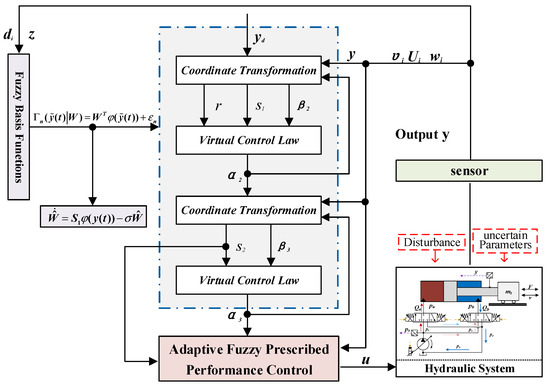
Figure 2.
Schematic diagram of the control framework.
Note: The control design, particularly the K-filter and the fuzzy logic system, inherently compensates for and mitigates the effects of sensor measurement noise present in the output signal y(t).
For the IMS nonlinear system, the following state transformation is performed:
In this formulation, for , represents the virtual control law to be synthesized. To mitigate the issue of ‘complexity explosion’ inherent in the standard backstepping procedure, each is passed through a first-order low-pass filter, yielding the filtered signal . This is the core mechanism of the DSC technique. The recursive controller is then systematically developed by integrating this DSC approach with adaptive control strategies.
The first step: Select the Lyapunov function.
Combined with the state transformation (27), the derivative of satisfies
where , , , and it is easy to know that
Conjunction with Yang’s inequality yields
where ; is a constant greater than zero.
By inserting Equation (31) into Equation (29), the derivative takes the following form:
Due to , combined with Yang ‘s inequality,
where , the positive constants and are introduced during the inequality scaling process, and denotes an unknown nonlinear function. The recursive design begins by formulating the virtual control law as follows:
where
As is available from Formula (8),
Collate to obtain the following:
Subsequently, the signal is passed through a first-order filter to obtain its smoothed version, . The filter is implemented as follows:
where is the filter time constant.
As is further available,
Substitute Equations (36)–(38) into Equation (35):
The second step: Select the following Lyapunov function.
The time derivative of the second error surface can be expressed as follows:
Then, the derivative of is
From the Formula (8), we can see that
The virtual control input structure is designed as follows:
Following the same DSC principle, a first-order filter is applied to the virtual control law . Its filtered output, denoted as , is introduced and governed by the following dynamics:
where is the filter time constant. Similarly, as is further available,
Substitute (41), (44) into (42):
The third step: Choose Lyapunov function.
Following the same procedure, the derivative for the third error surface, derived as , is
The derivative of is
Therefore, the controller of the design system is
Then, the derivative of can be written as
To address the system’s unknown nonlinear dynamics , an online approximator based on an FLS is integrated into the control architecture. This approximator models the uncertainty as
where is the vector of adjustable parameters, is the fuzzy basis function vector constructed from the tracking error, and denotes the inherent approximation error bounded.
In the stability analysis, the cross-term is encountered. Applying Young’s inequality, this term can be bounded as follows to facilitate the Lyapunov derivative analysis:
where defines the parameter estimation error between the ideal weight vector and its estimate .
To ensure bounded estimates and robust adaptation, the parameter vector is updated online via the following adaptive law with σ-modification:
It is worth noting that the adaptive law in (56) incorporates a σ-modification term to prevent the well-known issue of parameter drift in adaptive control. This leakage term ensures that the parameter estimates remain bounded even in the presence of measurement noise or during periods of low learning activity, thereby guaranteeing the overall robustness and stability of the closed-loop system.
The total Lyapunov function is constructed as follows:
In summary, it can be seen that the following formula is established:
To proceed, the following inequality is employed:
where
where and is a constant greater than zero and is a bounded function.
For the nonlinear function terms , in Equation (58), the following formula is established:
where .
A composite Lyapunov function candidate is adopted to rigorously analyze the stability of the system in the presence of unmodeled dynamics, defined as follows:
where .
Similarly, we can know that the derivative of is
where
Combined with the idea of supply function change, the derivative of satisfies
By the function , easily obtained inequality holds. Then, the derivative of can be written as follows:
Accordingly, a function needs to be designed satisfying the inequality
The specific form of the unknown function to be estimated is defined as follows:
In summary, the Lyapunov function we finally follow is
Its derivative satisfies
Since is a positive definite symmetric matrix, there exists a positive definite symmetric matrix such that
Inequality holds. To ensure stability, the time constants of the first-order filters used in each design step are chosen to satisfy
It can be seen from Formulas (58), (72), and (73) that
The following relation can be derived from the properties of the estimation error and Yang’s inequality:
Substituting Equations (74), (77) and (78) into Equation (73) obtains
where
In this context, the symbols and correspond to the smallest and largest eigenvalues of the relevant matrix.
Define the following compact set:
Designing the parameter, when and , , indicates that is an invariant set. That is, the initial value is selected, and for all , there is . Combinatorial (79), there is available
It can be seen that and adaptive parameter signals are bounded and stable. Further, is bounded stable; due to the boundedness of the input signal , it is easy to know that is bounded and stable. Then, it is uniformly bounded for all signals of the system.
4.2. Design of Oil Return Pressure Controller
In the case of a given load force, in order to determine the only reference pressure of the two chambers, a lower constant pressure will be set on the back pressure side to maintain the overall pressure at a lower level to save energy.
The rod cavity pressure controller needs to calculate the control input that makes the pressure track with a certain accuracy. Define the parameter vector .
Define the pressure tracking error variable and derive the following:
Taking A as the control input, according to the DCARC theory [21], the control law is as follows:
In the formula, the control law includes two parts, the adaptive model compensation term and robust feedback term . represents the lower bound of parameter and , and the selection condition of feedback gain will be given later.
Bring the controller (80) into Equation (79) to obtain
where
From Equation (81), can be designed to satisfy the following stabilization conditions:
In the formula, is any small design parameter.
The parameter vector is estimated online, and the estimated value is updated online by applying the adaptive law of discontinuous projection:
where is an adaptive diagonal matrix and is an adaptive function.
5. Experimental Verification
To validate the performance advantages of the proposed controller, a three-degree-of-freedom (3-DOF) heavy-duty manipulator testbed, centered on an independent metering hydraulic system, was constructed (see Figure 3). The hydraulic power was supplied by a Rexroth SYDFEE-20/071R (Horb am Neckar, Germany) electro-proportional pump, whose displacement was regulated via a pressure-flow compound control scheme. The inlet and outlet ports of the boom, arm, and bucket actuators were independently governed by dedicated Rexroth 4WREE-10 proportional servo valve from Rexroth company (Germany) proportional servo valves. For system feedback, actuator displacements were measured using NS-WY06-1000mm cable (Shanghai Tianmu company, Shanghai, China) sensors (with a measurement noise of ±0.5 mm), while load pressures were acquired via RPT8200-series (Shanghai Stedeford company, Shanghai, China) transducers (with a measurement noise of ±0.07 MPa).
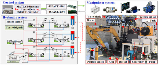
Figure 3.
Three-degree-of-freedom heavy-duty manipulator platform based on independent-metering hydraulic system. Adapted from [23].
The measurement and control framework was implemented using dSPACE rapid control prototyping. The control algorithm designed in Simulink was compiled into deployable code. Real-time monitoring and parameter tuning were facilitated by the ControlDesk 2018 software. At the hardware level, command signals to the pump and valves were output through a dS-4302 board to drive the manipulator, while sensor signals were simultaneously fed back to the controller via a dS-2004 board, closing the control loop. A consistent sampling period of 10 ms was maintained throughout the experiments.
The performance of the proposed controller was evaluated under the inherent measurement noise of the sensors (as specified in Section 4.1). Despite these non-ideal conditions, the controller successfully achieved precise trajectory tracking with the prescribed transient and steady-state performance, which underscores its inherent robustness to measurement uncertainties.
The prescribed performance bounds were configured with the function , and the scaling parameters were chosen as and .
The core control algorithm integrates an adaptive fuzzy mechanism with an extended state observer for the IMS. The observer gain was synthesized via Linear Matrix Inequality (LMI) techniques using the MATLAB 2022b LMI toolbox. Setting the symmetric matrices , the solver yielded the observer gain vector and the corresponding positive definite matrix :
The fuzzy subsystem employs Gaussian membership functions defined as , , and .
The fuzzy basis functions are consequently derived as follows:
To adjust the design parameters online, the following adaptive law is implemented:
Among them, and select the parameters , and the other parameters of the controller are set to the following: , , , , , , , , , . The time constant of the first-order filter is , .
The initial value of each state of the system is selected as
There are two controllers compared in this section to verify the effectiveness of the proposed control scheme.
C1: This is the controller proposed in this paper.
C2: This is a controller that lacks PPC, and the remaining control parameters are consistent with C1. The control law is
Taking the flat-ground condition of the manipulator as an example, the performance of the controller is compared according to the pulsating continuous and smooth bucket tip motion trajectory shown in Figure 4.
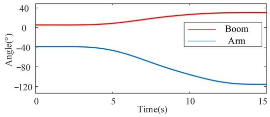
Figure 4.
Trajectory of flat-ground condition. Schemes follow the same formatting.
Figure 4 illustrates the desired pulsating and continuous bucket-tip motion trajectory used for the performance evaluation of the controllers under the flat-ground condition. This specific trajectory was designed to emulate a typical, challenging excavation cycle. It includes periods of smooth, continuous motion as well as sudden changes in direction and velocity (the ‘pulsating’ segments), which are representative of real-world operational commands. The purpose of employing such a trajectory is to rigorously test and demonstrate the controller’s ability to handle both smooth tracking and rapid transient responses. The subsequent experimental results (Figure 5, Figure 6, Figure 7, Figure 8, Figure 9 and Figure 10) are all based on tracking this reference trajectory.
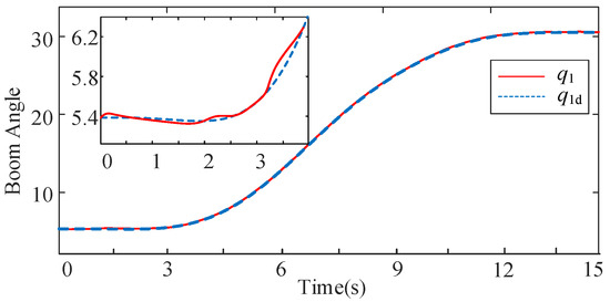
Figure 5.
The trajectory tracking effect of the boom under the C1 controller.
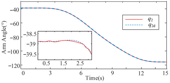
Figure 6.
The trajectory tracking effect of the stick under the C1 controller.
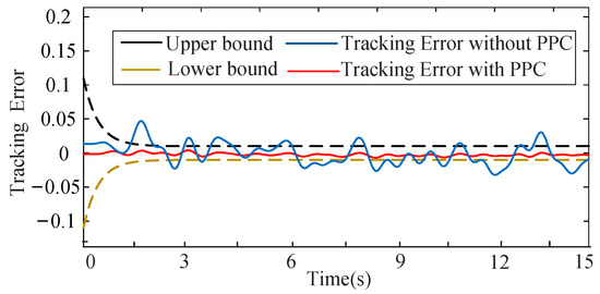
Figure 7.
The trajectory tracking error of the boom under different controllers.
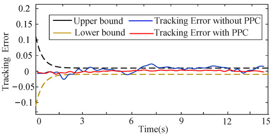
Figure 8.
The trajectory tracking error of the stick under different controllers.
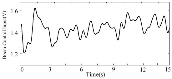
Figure 9.
The control input of the boom joint under the C1 controller.
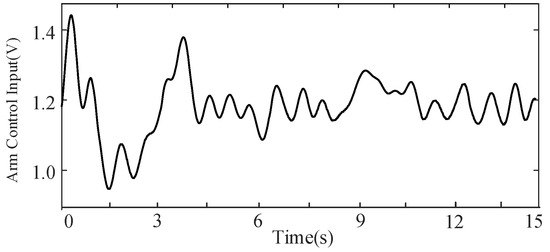
Figure 10.
The control input of the stick joint under the C1 controller.
Figure 5 and Figure 6 show the position tracking performance of the boom and arm joints under the C1 controller. It can be seen that the actual positions of the two joints can track the desired trajectory well. The tracking errors of the two controllers are compared as shown in Figure 7 and Figure 8. In order to ensure an objective quantitative comparison [25], the control performance of controllers C1 and C2 is further evaluated by using the maximum absolute value, mean value, and standard deviation of the tracking error as the measurement indicators. It can be seen from the experimental results that the transient and steady-state control performance of the proposed controller C1 is better than that of the C2 controller. The main reason is that the predetermined performance framework is introduced. At the same time, based on the K-filter as the extended state observer to observe the position state variable of the system, the FLS is used to perform feedforward compensation for the unmodeled error of the manipulator dynamics and the hydraulic system to improve the progressive tracking performance of the system. The control input is shown in Figure 9 and Figure 10, which show the real-time motion state of the bucket tip when the manipulator performs the trajectory tracking task. It can be clearly seen that the manipulator successfully completes the desired flat-ground trajectory, which verifies the feasibility of the proposed scheme.
Figure 5 and Figure 6 present the primary validation of the trajectory tracking performance of the proposed C1 controller. The results demonstrate that the integrated system, combining the K-filter state observer and the adaptive fuzzy controller, successfully achieves high-precision tracking of the desired trajectories for both the boom and arm joints under the standard operating conditions.
To quantitatively validate the critical role of the PPC framework, a comparative analysis between the proposed controller (C1) and a counterpart without PPC (C2) is presented in Figure 7 and Figure 8. The results conclusively show that only C1 guarantees that the tracking error remains within the user-defined, exponentially decaying performance bounds, thereby validating the theoretical PPC capability.
The quantitative superiority of the proposed C1 controller is unequivocally demonstrated in Table 1. For the boom joint, C1 reduces the MAE, STD, and ITAE by approximately 73%, 75%, and 82%, respectively, compared to the C2 controller. Similar significant improvements are observed for the arm joint. This quantitatively confirms that the proposed controller not only constrains the error within preset bounds but also significantly improves the absolute tracking precision and dynamic response across both transient and steady-state phases.

Table 1.
Quantitative performance indices for the flat-ground trajectory.
Based on the oil return pressure controller, the oil return pressure of the hydraulic cylinder is constrained, as shown in Figure 11; in the whole operation cycle, the oil return pressure of the system is controlled in a low range, which effectively reduces the pressure loss caused by the throttling of the oil return valve port and improves the energy utilization efficiency.
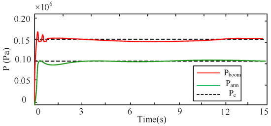
Figure 11.
Back pressure tracking performance of pressure controller.
Figure 11 provides direct experimental verification of the energy-saving capability of the proposed system. The dedicated oil return pressure controller, designed in Section 4.2, successfully maintains the rod cavity pressure at a low constant level, significantly reducing the throttling losses across the return-side valve orifice and thereby improving the overall system energy efficiency.
In order to further evaluate the generalization performance and robustness of the proposed control algorithm, two new motion trajectories are used for testing. As shown in Figure 12 and Figure 13, under the action of the C1 controller, the boom and the arm joint still show good tracking performance on two different forms of desired trajectories, and the actual position can accurately and smoothly follow the target motion. It can be seen that the manipulator can successfully complete different types and complexities of trajectory tasks. At the same time, as shown in Figure 14, the oil return pressure of the system is still stably limited to a lower range throughout the process, which significantly reduces the throttling loss and reflects a good energy-saving effect. The above results consistently show that the proposed control strategy has high feasibility and energy efficiency in different trajectory tasks.
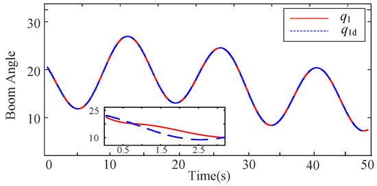
Figure 12.
The trajectory tracking effect of the boom under the C1 controller.
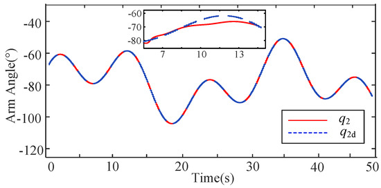
Figure 13.
The trajectory tracking effect of the stick under the C1 controller.
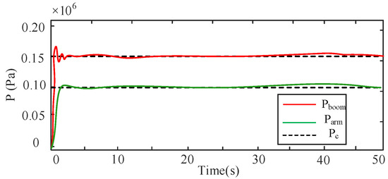
Figure 14.
Back pressure tracking performance of pressure controller.
To test the robustness and generalizability of the C1 controller beyond a single operating condition, it was subjected to more complex and demanding trajectories. As shown in Figure 12 and Figure 13, the controller maintains excellent tracking performance. Furthermore, Figure 14 confirms that the energy-saving pressure control remains effective. This consistent performance across diverse tasks robustly validates the controller’s practicality and adaptability.
The quantitative energy-saving effect of the proposed scheme is unequivocally demonstrated in Table 2. The dedicated pressure controller in C1 actively maintains the average return pressure at a low level for both actuators. For instance, under the flat-ground condition, the boom’s return pressure is reduced to 0.15 MPa (a 75% reduction) and the arm’s to 0.10 MPa (a 75% reduction), compared to their respective operational baselines without active pressure control. Similar significant reductions are achieved under the complex trajectory. This substantial lowering of the return pressure directly translates to a quadratic reduction in the throttling power loss across each return valve orifice, thereby providing definitive quantitative evidence for the improved energy efficiency claimed in this paper.
Table 2.
Quantitative analysis of energy-saving performance via return pressure.
In summary, the comprehensive experimental results from Figure 5, Figure 6, Figure 7, Figure 8, Figure 9, Figure 10, Figure 11, Figure 12, Figure 13 and Figure 14 collectively demonstrate the superior overall performance of the proposed C1 controller. The key achievements can be summarized in four aspects:
High-Precision Trajectory Tracking: As evidenced in Figure 5, Figure 6, Figure 12 and Figure 13, the C1 controller enables both the boom and arm joints to accurately follow the desired trajectories, including both standard and more complex paths.
Guaranteed Transient and Steady-State Performance: Figure 7 and Figure 8 provide definitive proof that the tracking error of the C1 controller is strictly constrained within the user-defined, exponentially decaying bounds of the prescribed performance function, fulfilling the core theoretical promise of the PPC methodology.
Effective Energy-Saving Capability: The functionality of the dedicated oil return pressure controller is successfully validated in Figure 11 and Figure 14, showing that the system back pressure is actively maintained at a low level, thereby reducing throttling losses and improving overall energy efficiency.
Robustness and Generalizability: The consistent and reliable performance of the C1 controller across different and more complex operational trajectories (Figure 12, Figure 13 and Figure 14), under realistic sensor noise and disturbances, underscores its robustness and practical applicability beyond a single specific task.
These results, taken together, confirm that the C1 controller successfully integrates the K-filter-based state observation, adaptive fuzzy compensation, and prescribed performance control into a cohesive framework that delivers high accuracy, robustness, and energy efficiency simultaneously.
6. Conclusions
This study shows that the predetermined performance control strategy based on adaptive output feedback proposed for the IMS significantly improves the system’s energy efficiency while achieving high-precision trajectory tracking. A K-filter is utilized, serving to accurately reconstruct the unmeasurable state quantities, and the dependence on speed and pressure sensors is effectively overcome. The FLS is used to compensate for the unmodeled dynamics and external disturbances online, which enhances the robustness of the system. Furthermore, the PPC theory is used to constrain the transient and steady-state performance of the tracking error to ensure the control accuracy. In addition, the application of the dynamic surface control method avoids the ‘computational explosion’ problem in backstepping control and improves the algorithm’s realizability. The specially designed oil return pressure controller maintains the back pressure at a low level, reducing the throttling loss of the oil return path and thereby improving the overall energy efficiency. Theoretical analysis and comparative experimental results show that the proposed control strategy can achieve excellent tracking performance and energy-saving effects at the same time in the presence of time-varying disturbance and parameter uncertainty, which provides a promising solution for the practical engineering application of the IMS.
The follow-up research can focus on optimizing the design and application of self-organizing Gaussian basis function vectors and gradually relax the existing assumptions in this paper to enhance the applicability and robustness of the algorithm. In addition, if it is further extended to stochastic systems, input saturation and output constraint processing mechanisms can be introduced, online optimization of control parameters can be realized by combining reinforcement learning, and the Monte Carlo method can be used to systematically evaluate the influence of different intensity uncertainties and noise on control quality, so as to comprehensively improve the tracking performance and reliability of the system.
Author Contributions
Conceptualization, Y.L.; Methodology, Y.L.; Software, Y.L.; Validation, Y.L.; Formal analysis, Y.L.; Investigation, Y.L.; Resources, Y.L.; Data curation, Y.L.; Writing—original draft, Y.L.; Writing—review & editing, Y.L.; Visualization, Y.L.; Supervision, X.Q.; Project administration, X.Q.; Funding acquisition, X.Q. All authors have read and agreed to the published version of the manuscript.
Funding
This research received no external funding.
Data Availability Statement
The original contributions presented in this study are included in the article. Further inquiries can be directed to the corresponding author.
Conflicts of Interest
Author Yuhe Li, employed by the Tianjin Research Institute of Construction Machinery Co., Ltd., Tianjin 300409, declares no financial or non-financial conflicts of interest related to the submitted work.
Abbreviations
| C1 | Proposed Controller (Adaptive Fuzzy Prescribed Performance Control) |
| C2 | Comparative Controller (Without Prescribed Performance Control) |
| DOF | Degree Of Freedom |
| DSC | Dynamic Surface Control |
| ESO | Extended State Observer |
| FLS | Fuzzy Logic System |
| IMS | Independent Metering System (or Load Port Independent Hydraulic System) |
| PPC | Prescribed Performance Control |
| PPF | Prescribed Performance Function |
| UUB | Uniformly Ultimately Bounded |
References
- Manring, N.D.; Fales, R.C. Hydraulic Control Systems; Wiley: New York, NY, USA, 2019. [Google Scholar]
- Shi, H.; Yang, H.; Gong, G.; Liu, H.; Hou, D. Energy saving of cutterhead hydraulic drive system of shield tunneling machine. Autom. Constr. 2014, 37, 11–21. [Google Scholar] [CrossRef]
- Chen, C.; Xiao, B.; Zhang, Y.; Zhu, Z. Automatic vision-based calculation of excavator earthmoving productivity using zero-shot learning activity recognition. Autom. Constr. 2023, 146, 104702. [Google Scholar] [CrossRef]
- Eriksson, B.; Palmberg, J.O. Individual metering fluid power systems: Challenges and opportunities. Proc. Inst. Mech. Eng. 2011, 225, 196–211. [Google Scholar] [CrossRef]
- Ramezani, M.; Tafazoli, S. Using Artificial Intelligence in Mining Excavators: Automating Routine Operational Decisions. IEEE Ind. Electron. Mag. 2021, 15, 6–11. [Google Scholar] [CrossRef]
- Hui, J.; Ling, J.; Yuan, J. Adaptive backstep controller with extended state observer for load following of nuclear power plant. Prog. Nucl. Energy 2021, 137, 103745. [Google Scholar] [CrossRef]
- Wang, C.; Liu, J.; Xin, L.; Li, G.; Pan, J. Design of full-order state observer for two-mass joint servo system based on the fixed gain filter. IEEE Trans. Power Electron. 2022, 37, 10466–10475. [Google Scholar] [CrossRef]
- Deng, W.; Yao, J. Extended-state-observer-based adaptive control of electrohydraulic servomechanisms without velocity measurement. IEEE/ASME Trans. Mechatron. 2019, 25, 1151–1161. [Google Scholar] [CrossRef]
- Santos, J.C.; Cuau, L.; Poignet, P.; Zemiti, N. Decoupled model predictive control for path following on complex surfaces. IEEE Robot. Autom. Lett. 2023, 8, 2046–2053. [Google Scholar] [CrossRef]
- Zhuang, H.; Sun, Q.; Chen, Z. Sliding mode control for electro-hydraulic proportional directional valve-controlled position tracking system based on an extended state observer. Asian J. Control 2021, 23, 1855–1869. [Google Scholar] [CrossRef]
- Li, Y.; Liu, Y.; Tong, S. Observer-based neuro-adaptive optimized control of strict-feedback nonlinear systems with state constraints. IEEE Trans. Neural Netw. Learn. Syst. 2022, 33, 3131–3145. [Google Scholar] [CrossRef]
- Won, D.; Kim, W.; Tomizuka, M. High-gain-observer-based integral sliding mode control for position tracking of hydraulic servo systems. IEEE/ASME Trans. Mechatron. 2017, 22, 2695–2704. [Google Scholar] [CrossRef]
- Zhou, Q.; Li, H.; Shi, P. Decentralized adaptive fuzzy tracking control for robot finger dynamics. IEEE Trans. Fuzzy Syst. 2015, 23, 501–510. [Google Scholar] [CrossRef]
- Chen, M.; Tao, G.; Jiang, B. Dynamic surface control using neural networks for a class of uncertain nonlinear systems with input saturation. IEEE Trans. Neural Netw. Learn. Syst. 2015, 26, 2086–2097. [Google Scholar] [CrossRef]
- Hua, C.; Guan, X. Output feedback stabilization for time-delay nonlinear interconnected systems using neural networks. IEEE Trans. Neural Netw. 2008, 19, 673–688. [Google Scholar]
- Chen, J.; Ai, C.; Kong, X. PID Control of Hydraulic Robotic Arm Based on Reinforcement Learning. IEEE Trans. Ind. Electron. 2025, 1–11. [Google Scholar] [CrossRef]
- Song, X.; Wu, C.; Song, S.; Tejado, I. Fuzzy wavelet neural adaptive finite-time self-triggered fault-tolerant control for a quadrotor unmanned aerial vehicle with scheduled performance. Eng. Appl. Artif. Intell. 2024, 131, 107832. [Google Scholar] [CrossRef]
- Yang, S.; Pan, Y.; Cao, L.; Chen, L. Predefined-Time Fault-Tolerant Consensus Tracking Control for Multi-UAV Systems with Prescribed Performance and Attitude Constraints. IEEE Trans. Aerosp. Electron. Syst. 2024, 60, 4058–4072. [Google Scholar] [CrossRef]
- Huang, X.; Biggs, J.D.; Duan, G. Post-capture attitude control with prescribed performance. Aerosp. Sci. Technol. 2020, 96, 105572–105589. [Google Scholar] [CrossRef]
- Ma, H.; Chen, M.; Feng, G.; Wu, Q. Disturbance-observer-based adaptive fuzzy tracking control for unmanned autonomous helicopter with flight boundary constraints. IEEE Trans. Fuzzy Syst. 2022, 31, 184–198. [Google Scholar] [CrossRef]
- Bechlioulis, C.; Rovithakis, G. Robust adaptive control of feedback liearizable IMO nonlinear systems with prescribed performance. IEEE Trans. Autom. Control 2008, 53, 2090–2099. [Google Scholar] [CrossRef]
- Ma, H.; Zhou, Q.; Li, H.; Lu, R. Adaptive prescribed performance control of a flexible-joint robotic manipulator with dynamic uncertainties. IEEE Trans. Cybern. 2021, 52, 12905–12915. [Google Scholar] [CrossRef]
- Chen, J.; Jiang, H.; Kong, X.; Ai, C. Mode Switching Control of Independent Metering Fluid Power Systems. ISA Trans. 2025, 158, 735–748. [Google Scholar] [CrossRef]
- Qi, X.; Li, C.; Ni, W.; Ma, H. A novel adaptive fuzzy prescribed performance congestion control for network systems with predefined settling time. Neural Comput. Appl. 2024, 36, 523–532. [Google Scholar] [CrossRef]
- Hua, C.; Liu, G.; Li, L.; Guan, X. Adaptive fuzzy prescribed performance control for nonlinear switched time-delay systems with unmodeled dynamics. IEEE Trans. Fuzzy Syst. 2017, 26, 1934–1945. [Google Scholar] [CrossRef]
- Wang, C.; Lin, Y. Decentralised adaptive dynamic surface control for a class of interconnected non-linear systems. IET Control Theory Appl. 2012, 6, 1172–1181. [Google Scholar] [CrossRef]
- Deng, W.; Zhou, H.; Zhou, J.; Yao, J. Neural network-based adaptive asymptotic prescribed performance tracking control of hydraulic manipulators. IEEE Trans. Syst. Man Cybern. Syst. 2023, 53, 285–295. [Google Scholar] [CrossRef]
- Guo, Q.; Zhang, Y.; Celler, B.G.; Su, S.W. Neural adaptive backstepping control of a robotic manipulator with prescribed performance constraint. IEEE Trans. Neural Netw. Learn. Syst. 2019, 30, 3572–3583. [Google Scholar] [CrossRef]
- Wang, S.; Yu, H.; Yu, J.; Na, J.; Ren, X. Neural-network-based adaptive funnel control for servo mechanisms with unknown dead-zone. IEEE Trans. Cybern. 2020, 50, 1383–1394. [Google Scholar] [CrossRef]
- Koivumäki, J.; Zhu, W.H.; Mattila, J. Energy-efficient and high-precision control of hydraulic robots. Control Eng. Pract. 2019, 85, 176–193. [Google Scholar] [CrossRef]
- Ding, R.; Zhang, J.; Xu, B.; Cheng, M. Programmable hydraulic control technique in construction machinery: Status, challenges and countermeasures. Autom. Constr. 2018, 95, 172–192. [Google Scholar] [CrossRef]


Disclaimer/Publisher’s Note: The statements, opinions and data contained in all publications are solely those of the individual author(s) and contributor(s) and not of MDPI and/or the editor(s). MDPI and/or the editor(s) disclaim responsibility for any injury to people or property resulting from any ideas, methods, instructions or products referred to in the content. |
© 2025 by the authors. Licensee MDPI, Basel, Switzerland. This article is an open access article distributed under the terms and conditions of the Creative Commons Attribution (CC BY) license (https://creativecommons.org/licenses/by/4.0/).