Abstract
In recent years, hydrothermal geothermal resources have been predominantly exploited through well cluster systems, achieving extensive commercial implementation. The efficient development of such systems remains critically dependent on the comprehensive characterization of regional geological conditions, as multiple subsurface parameters—including stratal thickness, structural relief, porosity–permeability distribution, and fault architecture—exert substantial control over reservoir performance. However, the effective integration of these geological factors to optimize well network configurations, balancing economic viability, power output, and other evaluation metrics to enhance heat extraction efficiency and delay thermal breakthrough, remains unresolved. This study aimed to identify the optimal well cluster for hydrothermal geothermal resources in the X region. Geological, drilling, and well-logging data were compiled to construct a region-specific geological model. A coupled numerical model of fluid flow and heat transfer was developed for a five-spot well pattern. System performances under two commonly applied injection-to-production ratios (2:3 and 1:4) and spatial configurations between injection and production wells were quantified. A multi-criteria evaluation framework integrating heat extraction power, injection–production pressure difference, and production temperature decline was implemented to holistically assess well cluster. An integrated weighting strategy combining subjective expertise and objective analytical criteria was implemented alongside the TOPSIS method to systematically identify the optimal wellfield configuration. Results demonstrate that Pattern 11, comprising three injection wells and two production wells, achieved superior comprehensive performance among 15 patterns, with heat extraction power 24.13 MW, and production temperature decline <1 °C and injection–production pressure difference <3 MPa.
1. Introduction
Geothermal energy, a critical clean and renewable resource, offers high efficiency, operational stability, and independence from seasonal, climatic, or diurnal variations. It primarily encompasses shallow geothermal systems, hydrothermal resources, and enhanced geothermal systems (EGS) [1,2,3]. In China, hydrothermal geothermal systems remain the dominant development pathway due to their technological maturity and practical feasibility, typically deployed in well cluster configurations to supply heating for residential complexes, hospitals, airports, and other infrastructure [4,5].
The X study area, situated in the Bohai Bay Basin of eastern China, hosts Ordovician karst reservoirs characterized by high single well productivity, low salinity, and favorable reinjection potential [6,7]. Multiphase tectonic activity has established multiple source–reservoir–cap assemblages, with extensive research and field trials confirming the viability of Ordovician thermal reservoirs [8,9,10]. Governed by climatic demands, the clustered well hydrothermal heating system operates on a four-month winter extraction cycle followed by an eight-month summer recovery period [11].
In clustered well systems, cold working fluid is injected into the subsurface via injection wells, undergoes heat exchange within the reservoir rock, and is subsequently extracted through production wells for space heating. This process involves coupled multiphysics interactions among thermal, hydraulic, and mass transport fields [12]. Previous studies have extensively investigated these coupled mechanisms; some simplified reservoirs as homogeneous porous media to evaluate parameters like well spacing and flow rates, while others focused on fracture-dominated multiphysics coupling [13]. However, emerging research emphasizes the critical influence of reservoir heterogeneity, challenging traditional homogeneous assumptions [14]. Although methods such as correlation length modeling have been employed to simulate subsurface property heterogeneity, they often fail to accurately represent site-specific lithological distributions, limiting their utility in field-scale development guidance [15,16,17].
The efficiency of well cluster hydrothermal systems is highly sensitive to well network geometry, necessitating optimized selection among numerous configurations [18,19,20]. Existing evaluation metrics—primarily focusing on hydraulic drawdown and thermal breakthrough timing—exhibit oversimplification. In practice, multi-criteria decision-making integrating diverse performance indicators (e.g., thermal output stability, energy consumption, and reservoir longevity) remains unresolved.
This study constructed a geological model of the X sector to delineate stratigraphic architecture and petrophysical property distributions. A five-spot well pattern geothermal extraction model, coupled with thermal–hydraulic simulations, was developed to evaluate 15 well configuration patterns. A hybrid subjective–objective weighting method (AHP-EWM) integrated with TOPSIS decision analysis was implemented to identify the optimal well network for X’s geothermal development.
2. Materials and Methods
The X study area spans 5000 m × 3800 m in the southeastern Bohai Bay Basin, with stratigraphic sequences encompassing the Quaternary, Minghuazhen Formation, Guantao Formation, Jurassic–Cretaceous, Carboniferous–Permian, and Ordovician units. Extensive data indicate significant geothermal potential in this region. The primary reservoir for geothermal exploitation comprises Ordovician platform facies carbonate lithologies, dominated by gray marl and limestone interbedded with thin layers of medium-gray calcareous mudstone and mudstone. Mid-to-lower intervals consist of dark-gray limestone and dolomitic limestone interspersed with carbonaceous mudstone and calcareous mudstone. A 500 m thick fractured zone serves as the principal aquifer, yielding geothermal fluids at 127 m3/h.
The geological model integrates structural geology, sedimentology, and stratigraphy, synthesizing data from geological surveys, drilling, well logging, and mud logging to characterize the three-dimensional spatial distribution, structural attributes, and reservoir parameters of subsurface formations. Utilizing single well geothermal reservoir top elevation data derived from well-log interpretations, the Kriging interpolation method was applied to reconstruct the three-dimensional spatial architecture of the thermal reservoir. Building upon this framework, a sequential Gaussian simulation was employed to develop the reservoir property model, incorporating porosity data from single well interpretations. Permeability distributions were subsequently derived through petrophysical correlations with porosity, thereby completing the geological model of the X sector.
Results reveal a westward-dipping thermal reservoir with top depths of 800–1100 m and basal depths of 1500–1650 m (shown in Figure 1). The reservoir exhibits pronounced stratigraphic heterogeneity in porosity (0.05–0.18) and permeability (0–5000 mD), with vertical distributions detailed in Figure 2.
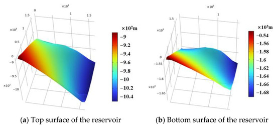
Figure 1.
The morphological features of the top surface and bottom surface of the reservoir.
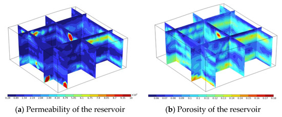
Figure 2.
The distribution characteristics of permeability and porosity in the reservoir.
3. Model Description
The computational framework is employed to analyze key parameters, aiming to capture evolving trends in production performance. To achieve a balance between computational efficiency and result reliability, the following simplifications are implemented:
- (1)
- Chemical interactions between reservoir rock and injected fluids are excluded;
- (2)
- Thermally induced stress variations are considered negligible;
- (3)
- Single-phase flow conditions governed by Darcy’s law are maintained throughout the extraction process;
- (4)
- Tiny cracks in the reservoir are not considered;
- (5)
- The wellbore geometry was reduced to a one-dimensional representation.
3.1. Governing Equation
The numerical model couples the conservation of mass, seepage dynamics, and thermal transport mechanisms. Through real-time coupling of key variables including fluid pressure, flow velocity, and temperature fields, the computational framework effectively captures the dynamic interactions between multiphase flow processes and heat transfer phenomena.
Seepage equations in the rock matrix follow [21]:
where ρf is the fluid density, kg/m3; S represents the storage coefficient of rock Pa−1; p is the pressure, Pa; t represents the time, s; u is the seepage velocity, m/s; k is the permeability, mD; μ represents the dynamic viscosity of the fluid, Pa·s; g represents the gravity term, m·s−2; and z represents the vertical direction.
Heat transfer in the rock matrix is as follows:
where (ρC)e is the effective enthalpy, J·K−1·m−3; λe represents the effective thermal conductivity, W(m·K)−1; cp,s and cp,f, respectively, represent the specific heat capacities of solid and fluid, J·(kg·K)−1; φ is the porosity; and λs and λf, respectively, represent the thermal conductivities of solid and fluid.
3.2. Geometric Model and Condition Settings
In this study, the reservoir is a hexahedron with a length and width of 1500 m and a height of approximately 600 m, buried about 1000 m underground. The exterior of the reservoir is a cuboid measuring 3000 m by 3000 m by 2000 m, which is used to represent surrounding rocks outside the reservoir. The well cluster configuration comprises five production units arranged in a 350 m spacing pattern. The well extends 1300 m underground from the top of the reservoir, with the detailed spatial geometry illustrated in Figure 3. The system operates on a periodic injection–production cycle spanning 360 days, partitioned into two distinct phases: an initial 120-day production period followed by a 240-day pressure restoration phase. This alternating production meets the actual working conditions of hydrothermal geothermal heating projects. To evaluate the long-term performance of well cluster configurations, a 50-year operational period is designed in the numerical model, which is implemented by repeating the base periodic injection–production cycle (120-day production phase + 240-day pressure restoration phase) for 50 consecutive times.
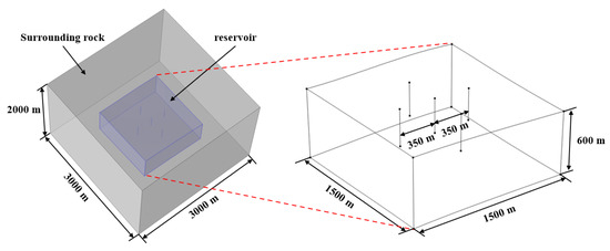
Figure 3.
Geometric characteristics of the model.
The neutral temperature layer in the X region maintains a baseline temperature of 20 °C, with geothermal temperatures increasing linearly with depth at a gradient of 0.032 °C/m. Reservoir pressure similarly exhibits a linear depth-dependent profile, characterized by a pressure gradient of 9800 Pa/m. Notably, permeability and porosity parameters were adopted from the petrophysical dataset established in Section 2 of the geological model. Additional detailed specifications of the model’s physical parameters, including thermal–hydraulic properties are comprehensively tabulated in Table 1.

Table 1.
Model physical parameter setting.
The entire model incorporates no-flow and adiabatic boundary conditions at the top and base, with the lateral boundaries constrained by constant pressure and constant temperature regimes. All five wells operate under constant mass flow rate conditions for both the production and injection phases.
The working fluid in the geothermal system is geothermal water (consistent with the actual hydrothermal resources in the X region), which is the dominant fluid medium for heat exchange and circulation in the Ordovician karst reservoir.
3.3. Verification of Grid Independence
The computational framework employs the finite element method (FEM) for governing equation resolution. The surrounding rock mass was discretized using unstructured free tetrahedral meshing, while the reservoir domain was similarly partitioned with tetrahedral elements, incorporating local mesh refinement around the five wells. To enhance numerical accuracy, global mesh densification was applied to the entire reservoir—the primary computational focus of this study (Figure 4).
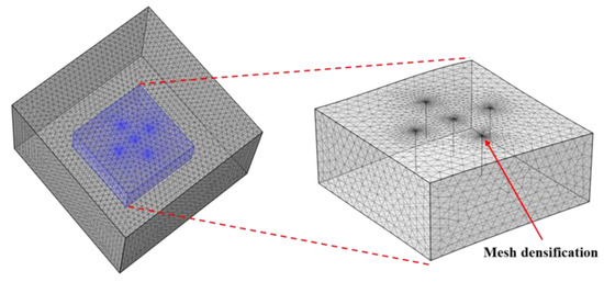
Figure 4.
Model grid meshing and densification.
A grid independence verification was conducted (Figure 5), demonstrating that a mesh configuration with 362,288 elements achieves optimal balance between computational accuracy and cost efficiency.
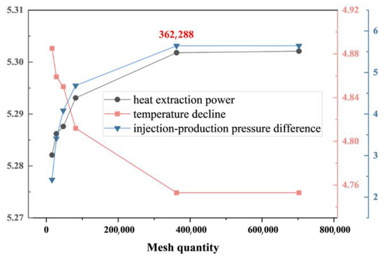
Figure 5.
Grid independence verification.
3.4. Governing Equation
A total of 15 distinct well pattern configurations were designed for the five-well development model in the X region. The spatial configurations of the 15 well patterns are explicitly illustrated in Figure 6 (In the figure, the blue points represent injection wells, and the red one represents production wells). These configurations incorporate two injection-to-production ratios, with a 1:4 ratio applied to the five well networks in the upper row (top tier) and a 2:3 ratio implemented across the lower two rows (middle and bottom tiers).
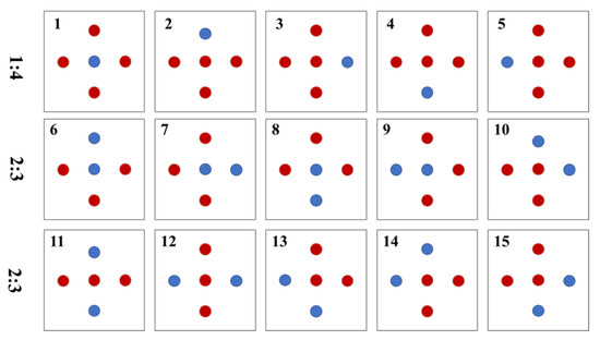
Figure 6.
Fifteen schemes for development with five-spot well pattern.
Notably, total production and injection rates were maintained constant across all well network configurations. This parity ensures comparative validity by isolating the effects of spatial arrangement and injection-to-production ratios on system performance.
3.5. Numerical Simulation Software and Solver Settings
The numerical simulation of coupled thermal–hydraulic processes in the geothermal reservoir was conducted using COMSOL Multiphysics—a widely recognized multiphysics simulation platform suitable for subsurface flow and heat transfer problems.
A transient implicit solver was used for time-dependent simulations (consistent with the 50-year operational period). For linear systems, the PARDISO direct solver was selected; for nonlinear iterations, the Newton–Raphson method was employed with a damping factor of 0.8. A variable time step was implemented; to capture transient pressure/temperature changes, 1-day steps for the first 30 days of each production/restoration phase, and 10-day steps for the remaining period to balance efficiency and accuracy were implemented. The maximum time step was constrained to 20 days to prevent numerical instability.
3.6. Model Validation
The model was validated using field production well temperatures from the X region. Owing to the absence of data from the initial years of on-site development, only the operational data from the sixth year were obtainable. As shown in Figure 7, the comparison between the field-measured data and the results calculated by this model indicates that the model is reliable.
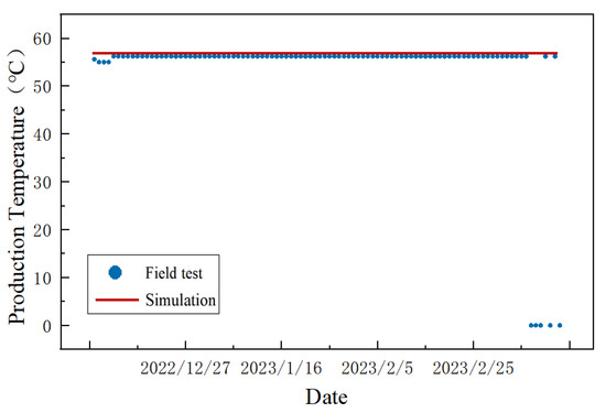
Figure 7.
Comparison between the field test data and simulated data.
4. Results and Discussions
4.1. Performance Evaluation Indicators
This study defines heat extraction power, injection–production pressure difference, and production temperature decline as evaluation indicators.
Heat extraction power refers to the total thermal energy continuously extracted from a reservoir per unit time by a geothermal system, typically quantified in megawatts (MW). This parameter serves as a critical metric for assessing the operational efficiency of geothermal field development. Heat extraction power calculated as follows:
where cf is the specific heat capacity of the fluid, J/(kg·k); qm is the injection mass flow velocity, kg/s; ρf is the density of fluid, kg/m3; and Tout and Tin are fluid average temperature of production and injection, °C.
The injection–production pressure difference refers to the pressure differential between injection and production wells in a geothermal system, measured in megapascals (MPa). This parameter serves as the primary driver for reservoir fluid circulation and is critical for sustaining heat exchange efficiency. The injection–production pressure difference is calculated as follows:
where pin is the injection pressure, Pa, and pout is the production pressure, Pa.
The production temperature decline denotes the progressive decrease in fluid temperature produced from geothermal wells over operational time, primarily attributable to inadequate thermal recharge of the reservoir or thermal interference from cold reinjected fluids. This phenomenon serves as a critical indicator for assessing the sustainable development potential of geothermal systems.
where Tout,initial is the initial production temperature, °C.
4.2. Performance of 15 Patterns
Figure 8 presents the 50-year cumulative heat extraction power for 15 well network configurations operating under intermittent production protocols (120-day active extraction followed by 240-day shut-in cycles annually). The system demonstrates sustained thermal outputs ranging between 21 MW and 24.5 MW, with three configurations exhibiting superior performance: Well Network 14 (24.15 MW), Well Network 11 (24.13 MW), and Well Network 2 (24.03 MW), while other configurations remain below 24 MW. Comparative analysis of injection-to-production ratios reveals distinct operational efficiencies—configurations with a 1:4 ratio (five networks) predominantly yield ≤ 23 MW (except Well Network 2 at 24.03 MW), whereas those with a 2:3 ratio (ten networks) consistently achieve higher outputs, maintaining 23–24 MW. This performance stratification underscores the critical influence of fluid reinjection strategies on long-term thermal sustainability in heterogeneous geothermal reservoirs.
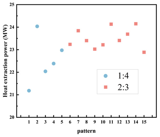
Figure 8.
Heat extraction power of 15 patterns.
Figure 9 illustrates the temperature decline across 15 well network configurations under intermittent production protocols (120-day active extraction followed by 240-day shut-in cycles annually) over a 50-year operational period. The system exhibits temperature reductions ranging from 0 to 5.1 °C, with the most significant declines observed in Well Network 1 (5.09 °C), Well Network 3 (3.55 °C), and Well Network 4 (3.11 °C), while other configurations show reductions below 2.4 °C. The comparative analysis of the two injection-to-production ratios reveals distinct thermal performance characteristics: among the five well networks operating under the 1:4 ratio, four configurations (excluding Well Network 2) exhibited temperature declines exceeding 2 °C, whereas the ten well networks utilizing the 2:3 ratio demonstrated superior thermal stability, with temperature reductions predominantly constrained below 2 °C. This pronounced divergence underscores the critical influence of fluid reinjection strategies on reservoir thermal equilibrium, where higher injection-to-production ratios (2:3) effectively mitigate thermal drawdown by maintaining enhanced hydraulic connectivity and heat replenishment rates.
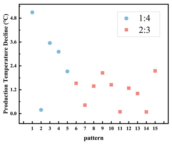
Figure 9.
Production temperature decline of 15 patterns.
Figure 10 presents the injection–production pressure differentials across 15 well network configurations under intermittent extraction protocols (120-day operational cycles annually) over a 50-year period. System-wide pressure differentials range from 2.4 MPa to 5.6 MPa, with the highest values observed in Well Network 5 (5.35 MPa), Well Network 2 (5.22 MPa), and Well Network 3 (4.58 MPa). Comparative analysis reveals that configurations with a 1:4 injection-to-production ratio exhibit significantly higher pressure differentials than those with a 2:3 ratio. This phenomenon arises from the system’s fixed total injection flux; fewer injection wells under the 1:4 ratio necessitate commensurately higher per-well injection rates, thereby inducing elevated wellhead pressures.
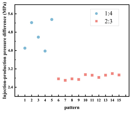
Figure 10.
Injection–production pressure difference of 15 patterns.
The preceding analysis demonstrates that no single well network configuration achieves superior performance across all three evaluation metrics. Consequently, identifying the optimal well layout among the 15 candidate configurations necessitates a more rigorous multi-criteria decision analysis framework. Such an approach must comprehensively reconcile trade-offs between heat extraction power, injection–production pressure difference, and production temperature decline.
4.3. Multi-Attribute Decision
To reconcile the three competing evaluation metrics and identify the optimal well network configuration, the implementation of a robust multi-attribute decision-making (MADM) method is imperative. The Technique for Order Preference by Similarity to an Ideal Solution (TOPSIS) provides a systematic framework for ranking alternatives based on their relative proximity to idealized positive and negative benchmark solutions. This method addresses the inherent multi-objective optimization challenges in geothermal system design through the following protocol.
The positive transformation and the alignment in the same trend of the original data are as follows:
where Xij represents the value of the j-th indicator of the i-th object. Then the distance between the best solution and the worst solution is calculated as follows:
where ωj is the weight of each indicator. Finally, the measure the degree of closeness between the evaluation objects and the optimal solution is calculated as follows:
where D−i is the distance from the i-th evaluation object to the negative ideal solution. D+i is the distance from the i-th evaluation object to the positive ideal solution.
The determination of weight values (wj) for each evaluation metric is crucial in comprehensive decision-making, as these weights critically influence the final outcomes. Traditional weighting methods can be categorized into subjective and objective approaches based on their computational principles. However, both methods exhibit inherent limitations: subjective weighting, reliant on expert experience, may introduce arbitrariness, while objective weighting, derived purely from mathematical models, risks misalignment with industry priorities, potentially yielding conclusions contradicting practical requirements. A combined weighting approach minimizes information loss during the weighting process, ensuring the derived weights closely approximate real-world operational priorities.
In this study, we implement this integrated subjective–objective weighting methodology, where the subjective weights are determined using the Analytic Hierarchy Process (AHP) to systematically incorporate expert judgment. Pioneered by American operations researcher Thomas L. Saaty in the 1970s, it is a multi-criteria decision analysis methodology that decomposes complex problems into hierarchical structures. By employing pairwise comparisons and mathematical operations—such as constructing judgment matrices and calculating weight prioritization—AHP integrates qualitative and quantitative analyses while ensuring logical coherence through consistency verification. The Analytic Hierarchy Process (AHP) decomposes a problem into distinct constituent factors based on their nature and the overall objective to be achieved. These factors are then aggregated and grouped into different levels according to their interrelationships, influences, and subordinate relationships, forming a multi-level analytical structural model. Ultimately, this process reduces the problem to determining the relative importance weights of elements at the lowest level (e.g., decision-making alternatives and measures) with respect to the highest level (the overall objective) or ranking their relative merits [22].
First, a hierarchical structure is established, comprising the top layer (the problem to be addressed), the middle layer (decision criteria), and the bottom layer (alternative solutions). Then, a pairwise comparison matrix A is constructed, where the element aij represents the comparison result of the i-th factor relative to the j-th factor. To calculate the approximate eigenvector, compute the n-th root of the product of elements in each row of matrix A, as follows:
Next, normalize Mi.
For consistency verification, calculate the eigenvalue of matrix A, as follows:
where λmax is the max of λ, ωi is the exact value of weight, and RI is the random consistency index (retrieved from standard tables based on the order n of matrix A).
If the consistency test is passed, the final weight is determined as follows:
In geothermal heating system optimization, where domain expertise serves as critical input, AHP translates subjective expert judgments into quantifiable decision parameters, thereby enhancing methodological rigor. The thermal extraction power is prioritized as the paramount criterion in our analysis, serving as the fundamental determinant of heating capacity to meet end-user thermal load demands—the central performance metric for geothermal heating system viability. Secondary consideration is given to the injection–production pressure differential, which governs energy consumption by maintaining hydraulic stability through regulated fluid circulation. The tertiary evaluation metric, production temperature decline, reflects the spatial uniformity of reservoir heat extraction and long-term sustainability of thermal recovery. The result is shown in Figure 11.
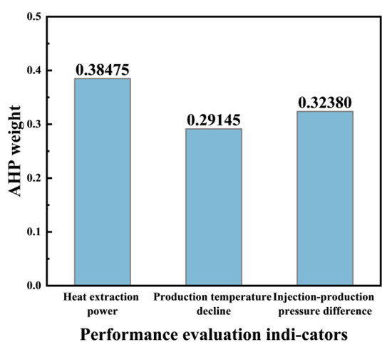
Figure 11.
Results of AHP weights of three performance evaluation indicators.
For objective weighting determination, the Entropy Weight Method (EWM) was employed as a data-driven weighting algorithm grounded in information entropy theory. This method autonomously calculates criterion weights based on the dispersion degree of dataset values across each metric, thereby circumventing subjective biases through its purely mathematical formulation.
First, calculate the feature proportion of the i-th object under the j-th criterion.
where bij denotes the standardized data of the j-th indicator for the i-th evaluation object. In this study, j = 3 and i = 15. Next, calculate the entropy value of the j-th indicator.
Calculate the divergence coefficient gj.
Finally, calculate the weight coefficient.
The result is shown in Figure 12.
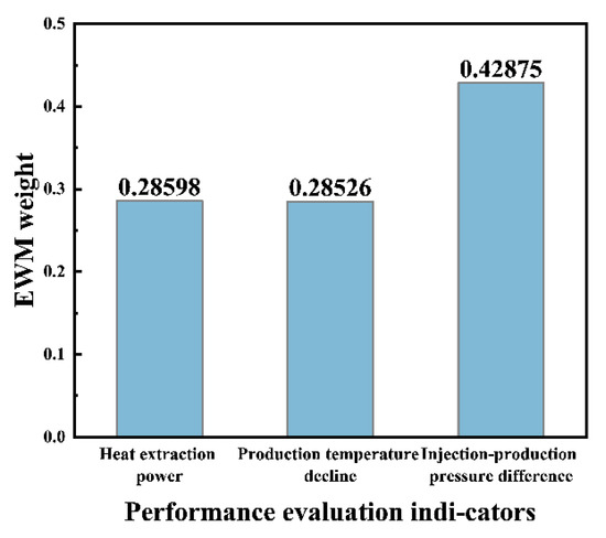
Figure 12.
Results of EWM weights of three performance evaluation indicators.
The comprehensive weight is calculated as follows:
where αj is the subjective weight from AHP. βj is the objective weight from EWM, as calculated above.
The results of the combined weight calculation are presented in Table 2. Herein, the injection–production pressure difference has the greatest weight (0.3753), followed by the heat extraction power (0.3342), and the production temperature decline comes last (0.2905).
Table 2.
Weight calculation result.
By integrating the hybrid subjective–objective weighting (AHP-EWM) values into the TOPSIS methodology, the Positive Ideal Solution Distance (PISD), Negative Ideal Solution Distance (NISD), and Comprehensive Score Index (CSI) were computed (Table 3). Analytical outcomes confirm that Pattern 11 achieves the superior integrated performance.
Table 3.
Calculation results of the TOPSIS evaluation method.
5. Conclusions
To obtain the optimal well pattern in the X area, this study constructed a geological model of the region, established a hydrothermal-coupled geothermal extraction model, and implemented a multi-criteria decision analysis to evaluate 15 well configurations, ultimately identifying the optimal solution. Key conclusions are as follows:
The Ordovician karst reservoir in the X area exhibits substantial thickness, well-developed porosity, and favorable permeability, confirming its viability as a high-productivity thermal resource.
Among the three thermal performance metrics, the injection–production pressure differential holds the highest priority, followed by the heat extraction rate, with the production temperature decline ranked as the tertiary consideration.
For the five-spot development configuration in the X area hydrothermal geothermal system, Pattern 11 has been identified as the multi-criteria-optimized solution, demonstrating superior thermal–hydraulic performance and long-term sustainability under the hybrid AHP-EWM/TOPSIS evaluation framework.
Author Contributions
Conceptualization, X.L., J.Y., G.W., and Q.W.; methodology, J.Y.; software, X.L. and J.Y.; validation, G.W. and Q.W.; formal analysis, X.L., J.Y., and S.L.; investigation, G.W. and Q.W.; resources, X.L.; data curation, Q.C.; writing—original draft, J.Y.; writing—review and editing, G.W. and Q.W.; visualization, J.Z.; supervision, X.L.; project administration, S.L.; and funding acquisition, Q.C. and J.Z. All authors have read and agreed to the published version of the manuscript.
Funding
The authors would like to acknowledge the National Natural Science Foundation of China (Grant Nos. 52304057, U24B2032), China National Postdoctoral Program for Innovative Talents (Grant No. BX20230428), National Natural Science Fund for Distinguished Young Scholars of China (Grant No. 52125401), Program of Introducing Talents of Discipline to Chinese Universities (111 Plan) (Grant Nos. B17045, B25049), and the Science Foundation of China University of Petroleum, Beijing (Grant Nos. 2462023XKBH016, 2462024BJRC018).
Data Availability Statement
The original contributions presented in this study are included in the article. Further inquiries can be directed to the corresponding author.
Acknowledgments
The authors gratefully acknowledge the technical support provided by CNOOC (China) Ltd. Beijing New Energy Branch for supplying geological and drilling data of the X region. Special thanks are extended to the State Key Laboratory of Petroleum Resources and Engineering at China University of Petroleum for facilitating the numerical simulation experiments.
Conflicts of Interest
Authors Xiangchun Li and Qian Wei were employed by the CNOOC (China) Ltd. The remaining authors declare that the research was conducted in the absence of any commercial or financial relationships that could be construed as a potential conflict of interest.
References
- Bertani, R.J.G. Geothermal power generation in the world 2010–2014 update report. Geothermics 2016, 60, 31–43. [Google Scholar] [CrossRef]
- Wang, G.; Liu, Y.; Zhu, X.; Zhang, W. Current Status and Development Trends of Geothermal Resources in China. Earth Sci. Front. 2020, 27, 1–9. [Google Scholar] [CrossRef]
- Wang, G.; Zhang, W.; Lin, W.; Liu, F.; Zhu, X.; Liu, Y.; Li, J. Research on formation mode and development potential of geothermal resources in Beijing-Tianjin-Hebei region. Geol. China 2017, 44, 1074–1085. [Google Scholar] [CrossRef]
- Wu, A.; Ma, F.; Wang, G.; Liu, J.; Hu, Q.; Miao, Q. A study of deep-seated karst geothermal reservoir exploration and huge capacity geothermal well parameters in Xiongan New Area. Acta Geosci. Sin. 2018, 39, 523–532. [Google Scholar] [CrossRef]
- Wang, F.; Cai, W.; Wang, M.; Gao, Y.; Liu, J.; Wang, Z.; Xu, J. Research Status and Prospect of Geothermal Heating Technology. J. Refrig. 2021, 42, 14–22. [Google Scholar] [CrossRef]
- Xiao, J.; Ji, H.; Hua, N.; Fang, C.; Li, H.; Ma, P. Sedimentary Facies Characteristics and Evolution of the Ordovician in the Dongpu Area, Bohai Bay Basin. Lithol. Reserv. 2016, 28, 78–87. [Google Scholar] [CrossRef]
- Wang, X.; Mao, X.; Mao, X.; Li, K. Characteristics and classification of the geothermal gradient in the Beijing–Tianjin–Hebei Plain, China. Math. Geosci. 2020, 52, 783–800. [Google Scholar] [CrossRef]
- Guo, X.; He, S.; Liu, K.; Shi, Z.; Bachir, S. Modelling the petroleum generation and migration of the third member of the Shahejie Formation (Es3) in the Banqiao Depression of Bohai Bay Basin, Eastern China. J. Asian Earth Sci. 2011, 40, 287–302. [Google Scholar] [CrossRef]
- Qiu, N.; Zuo, Y.; Zhou, X.; Li, C. Geothermal regime of the Bohai offshore area, Bohai Bay basin, North China. Energy Explor. Exploit. 2010, 28, 327–350. [Google Scholar] [CrossRef]
- Xu, H.; Zhang, J. Prospects for Geothermal Energy Utilization in Oilfields of the Bohai Rim and Beijing-Tianjin Region. Acta Sci. Nat. Univ. Pekin. (Nat. Sci. Ed.) 2012, 36, 182–185. [Google Scholar] [CrossRef]
- Li, S.; Wang, G.; Zhou, M.; Song, X.; Shi, Y.; Yi, J.; Zhao, J.; Zhou, Y. Thermal performance of an aquifer thermal energy storage system: Insights from novel multilateral wells. Energy 2024, 294, 130915. [Google Scholar] [CrossRef]
- Pandey, S.; Chaudhuri, A.; Kelkar, S. A coupled thermo-hydro-mechanical modeling of fracture aperture alteration and reservoir deformation during heat extraction from a geothermal reservoir. Geothermics 2017, 65, 17–31. [Google Scholar] [CrossRef]
- Xu, F.; Ma, T.; Tang, Y.; Song, X.; Shi, Y. Evaluation of heat extraction performance for vertical multi-fractures in enhanced geothermal system. Energy Sources Part A Recovery Util. Environ. Eff. 2025, 47, 9215–9236. [Google Scholar] [CrossRef]
- Liu, G.; Wang, G.; Zhao, Z.; Ma, F. A new well pattern of cluster-layout for deep geothermal reservoirs: Case study from the Dezhou geothermal field, China. Renew. Energy 2020, 155, 484–499. [Google Scholar] [CrossRef]
- Shi, Y.; Yang, Z.; Peng, J.; Zhou, M.; Song, X.; Cui, Q.; Fan, M. CO2 storage characteristics and migration patterns under different abandoned oil and gas well types. Energy 2024, 292, 130545. [Google Scholar] [CrossRef]
- Kane, E.; Leeuwenburgh, O.; Joosten, G.; Daniilidis, A.; Bruhn, D. Flexible well patterns and cashflow optimisation on large-scale geothermal field development. Renew. Energy 2025, 243, 122494. [Google Scholar] [CrossRef]
- Wang, J.; Zhao, Z.; Liu, G.; Xu, H. A robust optimization approach of well placement for doublet in heterogeneous geothermal reservoirs using random forest technique and genetic algorithm. Energy 2022, 254, 124427. [Google Scholar] [CrossRef]
- Cai, X.; Liu, Z.; Xu, K.; Li, B.; Zhong, X.; Yang, M. Numerical simulation study of an Enhanced Geothermal System with a five-spot pattern horizontal well based on thermal-fluid-solid coupling. Appl. Therm. Eng. 2025, 258, 124649. [Google Scholar] [CrossRef]
- Hou, X.; Chen, C.; Zhong, X.; Nie, S.; Wang, Y.; Tu, G. Numerical simulation study of closed-loop geothermal system well pattern optimisation and production potential. Appl. Therm. Eng. 2023, 231, 120864. [Google Scholar] [CrossRef]
- Gudala, M.; Govindarajan, S.K.; Yan, B.; Sun, S. Numerical investigations of the PUGA geothermal reservoir with multistage hydraulic fractures and well patterns using fully coupled thermo-hydro-geomechanical modeling. Energy 2022, 253, 124173. [Google Scholar] [CrossRef]
- Cui, Q.; Shi, Y.; Yang, Z.; Song, X.; Peng, J.; Liu, Q.; Fan, M.; Wang, L. An integrated system of CO2 geological sequestration and aquifer thermal energy storage: Storage characteristics and applicability analysis. Energy Convers. Manag. 2024, 318, 118876. [Google Scholar] [CrossRef]
- Franek, J.; Zmeškal, Z. A model of strategic decision making using decomposition SWOT-ANP method. In Proceedings of the Financial Management of Firms and Financial Institutions 9th International Scientific Conference Proceedings (Part I–III), Ostrava, Czech Republic, 9–10 September 2013; VŠB–Technical University of Ostrava: Ostrava, Czech Republic, 2013; pp. 172–180. [Google Scholar]


Disclaimer/Publisher’s Note: The statements, opinions and data contained in all publications are solely those of the individual author(s) and contributor(s) and not of MDPI and/or the editor(s). MDPI and/or the editor(s) disclaim responsibility for any injury to people or property resulting from any ideas, methods, instructions or products referred to in the content. |
© 2025 by the authors. Licensee MDPI, Basel, Switzerland. This article is an open access article distributed under the terms and conditions of the Creative Commons Attribution (CC BY) license (https://creativecommons.org/licenses/by/4.0/).