Multi-AGV Collaborative Task Scheduling and Deep Reinforcement Learning Optimization Under Multi-Feature Constraints

Abstract

To address the challenges of low efficiency, instability, and difficulties in meeting multiple constraints simultaneously in multi-AGV (Automated Guided Vehicle) task scheduling for intelligent manufacturing and logistics, this paper introduces a scheduling method based on multi-feature constraints and an improved deep reinforcement learning (DRL) approach (Improved Proximal Policy Optimization, IPPO). The method integrates multiple constraints, including minimizing task completion time, reducing penalty levels, and minimizing scheduling time deviation, into the scheduling optimization process. Building on the conventional PPO algorithm, several enhancements are introduced: a dynamic penalty mechanism is implemented to adaptively adjust constraint weights, a structured reward function is designed to boost learning efficiency, and sampling bias correction is combined with global state awareness to improve training stability and global coordination. Simulation experiments demonstrate that, after 10,000 iterations, the minimum task completion time drops from 98.2 s to 30 s, the penalty level decreases from 130 to 82, and scheduling time deviation reduces from 12 s to 0.5 s, representing improvements of 69.4%, 37%, and 95.8% in the same scenario, respectively. Compared to genetic algorithms (GAs) and rule-based scheduling methods, the IPPO approach demonstrates significant advantages in average task completion time, total system makespan, and overall throughput, along with faster convergence and better stability. These findings demonstrate that the proposed methodology enables effective multi-objective collaborative optimization and efficient task scheduling within complex dynamic environments, holding significant value for intelligent manufacturing and logistics systems.

1. Introduction

With the rapid development of artificial intelligence, machine learning, DRL, and neural networks, intelligent logistics scheduling systems have emerged as vital tools for enhancing production and transportation efficiency [1,2]. The essence of a scheduling system lies in the efficient allocation and utilization of production and logistics resources, aiming to improve overall operational performance by reducing waiting times and transportation cycles. Traditional research often frames scheduling problems as queuing and service issues, optimizing efficiency and effectiveness by configuring service station numbers and durations appropriately [3]. Researchers commonly use mathematical modeling to abstractly describe scheduling processes and enhance system performance through optimization models, improved algorithms, and strategy design.

AGVs are widely adopted as scheduling carriers in intelligent manufacturing and logistics, valued for their high flexibility, precision, and rapid response [4]. Research on multi-AGV scheduling has focused on three main areas: the development of scheduling models, optimization of scheduling algorithms, and the design of scheduling strategies [5]. The adaptability of traditional rule-based scheduling methods is inherently limited when dealing with increasingly dynamic and complex operational environments. Meta-heuristic algorithms can enhance optimization performance to some extent but often suffer from cumbersome parameter tuning and insufficient generalization [6,7,8]. In recent years, artificial intelligence methods, including reinforcement learning and neural network models, have been increasingly applied to multi-AGV scheduling for task allocation and path planning. Despite achieving some progress, these approaches still face challenges such as modeling difficulties, limited algorithmic diversity, and insufficient convergence stability [7,9].

Accurately characterizing environmental features is crucial for the efficiency and stability of scheduling systems. Studies have shown that scheduling environments can generally be divided into static and dynamic features [10,11]. Static features describe fixed spatial layouts and location points, while dynamic features involve workstation transfers and obstacle movements. Distinguishing and constraining different feature points in complex environments to mitigate the uncertainty introduced by dynamic variations has become an important research direction for improving scheduling efficiency [12,13,14,15]. Existing studies have attempted to optimize feature extraction using environmental geometric constraints, stage-wise calibration, and time-segmented recognition, along with leveraging AGV sensors and multi-dimensional path scanning for environmental modeling [16,17,18,19,20]. However, the accuracy of feature recognition in complex environments remains limited, restricting the generalization and real-time performance of scheduling models [21,22].

To enhance the adaptability and learning efficiency of scheduling models in dynamic environments, researchers have proposed guiding the training process of DRL models through multiple constraints, thereby reducing the search space and accelerating convergence [7,23]. In multi-AGV scheduling, common constraints include battery levels, task allocation, system states, environmental factors, and scheduling rules [24,25,26]. However, as the number of AGVs increases and the environment becomes more complex, constraints tend to become increasingly diverse and dynamic, posing higher demands on the real-time performance and robustness of scheduling algorithms.

In summary, existing multi-AGV scheduling methods still face limitations such as model homogeneity, poor generalization, and insufficient adaptability to dynamic environments. To address these challenges, this paper proposes a multi-AGV task scheduling method based on multi-feature constraints and an improved DRL approach (IPPO). The method incorporates minimum task completion time, penalty degree, and scheduling time deviation as core constraint features, and constructs a DRL model integrated with multi-feature constraints. Additionally, a dynamic penalty mechanism, a structured reward function, and sampling bias correction are introduced to achieve efficient scheduling and stable convergence in complex environments. Experimental validation on a simulation platform demonstrates significant performance improvements and robust stability, providing an effective solution for multi-AGV scheduling in intelligent manufacturing and logistics systems.

Current research on multi-AGV scheduling faces three main limitations: traditional methods struggle to achieve coordinated optimization of efficiency, stability, and multiple constraints in complex dynamic environments; existing reinforcement learning algorithms exhibit slow convergence and unstable training when handling multi-objective constraint problems; particularly, there is a lack of systematic modeling and coordinated optimization frameworks for multi-feature constraints such as task time, penalty degree, and time deviation, which severely restricts the effectiveness of intelligent scheduling systems in real industrial scenarios.

This study aims to systematically address the coordinated optimization of multi-feature constraints by constructing a multi-AGV collaborative scheduling framework based on Improved Proximal Policy Optimization (IPPO). Specific objectives include: establishing a deep reinforcement learning model that integrates multiple constraint features, designing dynamic penalty mechanisms and structured reward functions to enhance learning efficiency, and validating the comprehensive performance improvement of this method in scheduling efficiency, stability, and constraint satisfaction through simulation experiments, thereby providing an innovative solution for intelligent scheduling in complex industrial environments.

2. Research Method

2.1. Feature Constraint Optimization

Optimizing performance in AGV scheduling systems centers on the effective management of three critical constraints: minimum task time, penalty degree, and scheduling time deviation. First, the minimum task time constraint ensures tasks are completed within a set period, thereby preventing efficiency losses from delays. Then, the penalty degree constraint employs a penalty mechanism to curb violations of priority rules or improper resource allocation, thereby enhancing fairness and resource utilization. Third, the scheduling time deviation constraint aims to minimize differences between actual and planned schedules, thus improving system stability and predictability. By integrating these three constraints, the AGV scheduling system can achieve efficient and stable task allocation and path planning in complex, dynamic environments, balancing efficiency and fairness to meet the diverse needs of industrial applications.

2.1.1. Minimum Task Time Constraint

In multi-task scheduling and resource allocation, the minimum task time constraint is applied to guarantee that the actual completion time for any task remains above a designated minimum value. By imposing this limit, the constraint preserves basic execution efficiency, preventing delays caused by excessive resource dispersion or poor scheduling, and thereby enhancing the system’s responsiveness and processing capacity. In practical applications, this constraint is widely used in manufacturing, logistics distribution, and computational task scheduling. It optimizes resource allocation, reduces idle and waiting times, lowers operational costs, and further improves system throughput and overall operational efficiency.

For AGV task execution, the minimum task time constraint can be defined as follows. Let $T_i$ denote the completion time of the i-th AGV, $T_{\max }$ the maximum completion time among all AGVs, n the total number of AGVs, $\zeta$ a weighting coefficient, and $T_{avg}$ the average task completion time. Based on these definitions, the constraint can be expressed as depicted in Equation (1):

$$\left\{\begin{array}{l}{T}_{\mathit{max}}=\mathit{max}\left(T_1,T_2,\dots ,T_n\right)\hfill \\ T_{\mathit{avg}}={\displaystyle \frac{1}{n}}{\displaystyle {\sum }_{i=1}^n{T}_i}\hfill \\ T_{\mathit{max}}\le \zeta T_{\mathit{avg}}\hfill \end{array}\right.$$

(1)

where $T_{\max }\le \zeta T_{\mathit{avg}}$ represents that the maximum completion time $T_{\max }$ should not exceed the weighted average time $\zeta T_{\mathit{avg}}$. The weighting coefficient $\zeta$ is generally greater than or equal to 1, representing the tolerance for the maximum completion time. When $\zeta =1$, it implies that all AGVs must complete their tasks simultaneously; when $\zeta >1$, a certain variation in task completion times is permitted.

2.1.2. Penalty Degree Constraint

The penalty degree in DRL guides agent behavior by imposing a cost for non-compliance with predefined rules or constraints, thus encouraging AGVs to operate within established boundaries. This is achieved by integrating penalty terms into the reward function: whenever an agent’s action violates a constraint, a corresponding penalty is imposed, thereby reducing the expected return for that action. This design effectively directs the agent’s exploration process, thereby accelerating the learning of optimal, constraint-adhering strategies and enhancing overall adaptability and robustness in complex settings. To design the penalty degree constraint, the constraint optimization problem is first defined. Let the objective function $f\left(x\right)$ represent the target for minimization, with x denoting the optimization variables. A set of constraint conditions is then specified, as expressed in Equation (2):

$$\left\{\begin{array}{l}{g}_i\left(x\right)\ge 0, i=1,2,\dots ,p\hfill \\ h_j\left(x\right)=0, j=1,2,\dots ,q\hfill \end{array}\right.$$

(2)

To address solutions that violate these constraints, a penalty function $P\left(x\right)$ is introduced. Specifically, $P\left(x\right)$ = 0 when the optimization variables satisfy the constraints. Otherwise, $P\left(x\right)$ > 0 and increases as the degree of constraint violation grows. Accordingly, the expression of the penalty function is given in Equation (3):

$$\left\{\begin{array}{l}G\left[g_i\left(x\right)\right]=\max {\left(0,-g_i\left(x\right)\right)}^{\alpha },\alpha \ge 1\hfill \\ H\left[h_j\left(x\right)\right]={\left|h_j\left(x\right)\right|}^{\beta },\beta \ge 1\hfill \\ P\left(x\right)={\displaystyle {\sum }_{i=1}^{p}G\left[g_i\left(x\right)\right]}+{\displaystyle {\sum }_{j=1}^{q}H\left[h_j\left(x\right)\right]}\hfill \end{array}\right.$$

(3)

where $G\left[g_i\left(x\right)\right]$ represents the penalty term for inequality constraints, and $H\left[h_j\left(x\right)\right]$ represents the penalty term for equality constraints. The penalty degree function is then incorporated into the objective function $F\left(x\right)$, as shown in Equation (4). Depending on whether the optimization variables satisfy the constraints, the penalty function induces a corresponding transformation of the objective function:

$$F\left(x\right)=f\left(x\right)+\mu P\left(x\right)$$

(4)

where μ denotes the penalty parameter. As the penalty parameter μ approaches infinity, the penalty function P(x) is driven to infinity, ensuring that the minimum of F(x) converges to the solution that satisfies the constraint conditions.

2.1.3. Scheduling Time Deviation Constraint

In AGV scheduling, the time deviation constraint is vital for ensuring timely task completion. Time deviation refers to the difference between an AGV’s actual task completion time and the specified latest completion time. If an AGV fails to finish a task by its deadline, a time deviation occurs, potentially causing production delays and reducing overall efficiency. To manage time deviation effectively, scheduling models typically include a time deviation penalty function that imposes penalties for overtime behavior. By optimizing scheduling strategies to minimize time deviation, the operational efficiency and reliability of the AGV system can be substantially improved.

In a task scheduling system, let $t_{actual}$ denote the actual completion time of a task executed by an AGV, and $t_{due}$ represent the specified latest completion time for the task. The scheduling time deviation $t_{actual}$ is defined as shown in Equation (5): if $t_{actual}\le t_{due}$, the deviation is zero; if $t_{actual}>t_{due}$, the deviation equals the time delay.

$$T_{\mathit{deviation}}=\max \left(0,t_{actual}-t_{due}\right)$$

(5)

The scheduling model incorporates a time deviation penalty function. In AGV scheduling models, a generalized penalty function serves as a core optimization mechanism to effectively control time deviation and ensure timely task completion. This function is defined as shown in Equation (6), where $\alpha$ is the penalty coefficient ($\alpha >0$) and $k$ is the penalty exponent ($k\ge 1$), which together regulate the overall penalty intensity and control the form and severity of the penalty as the deviation increases.

$$P\left(T_{\mathit{deviation}}\right)=\alpha ·T_{\mathit{deviation}}^k$$

(6)

By adjusting the value of $k$, the penalty function can be flexibly tailored to different scheduling strategies. When $k=1$, the penalty exhibits a linear relationship with the deviation, aiming to minimize the total delay time. When $k=2$, the penalty increases quadratically, more severely penalizing larger deviations to enhance system stability. When $k>2$ or an exponential form is adopted, the penalty rises sharply, striving to eliminate overtime occurrences as much as possible. This approach is suitable for scenarios with extreme time sensitivity. In summary, the final optimization objective is to minimize the total penalty value across all tasks, as illustrated in Equation (7):

$$Minimize J={{\displaystyle \sum _{i=1}^N\alpha ·\left(T_i\right)}}^k$$

(7)

where N represents the total number of tasks. This function offers excellent differentiability and adaptability, enabling seamless integration into gradient-based or reinforcement learning scheduling frameworks, thereby significantly enhancing the timeliness and operational reliability of the AGV system.

2.2. Improved DRL Scheduling Model

2.2.1. Multi-Feature Constraint Relationships

Multi-AGV task allocation scheduling must not only assign tasks but also enhance allocation efficiency and optimize scheduling strategies to minimize logistics costs. Leveraging advances in artificial intelligence, a feature-constrained scheduling method that employs deep reinforcement learning (DRL) is proposed to achieve guided optimization, thereby enhancing training efficiency. The DRL framework captures data such as system states, AGV quantities, spatial information, and actions as responses to environmental stimuli. The datasets obtained from these interactions are collected and utilized for model training. This training process incorporates reward-penalty functions, objective functions, and feature constraint functions applied to the sample data, ultimately leading to the optimization and derivation of efficient scheduling policies.

In the scheduling system, feature constraints are the primary drivers influencing DRL. These constraints include: minimizing total task completion time, optimizing penalty severity, and reducing scheduling time deviations.

These conditions are employed as feature constraints for the AGV scheduling system. Reinforcement learning iteratively processes data related to system states, actions, rewards, transition probabilities, and discount factors. By integrating neural network models from deep learning and incorporating multi-feature constraints, the system effectively accomplishes AGV scheduling tasks.

Multi-feature constraints are integrated into the DRL framework by optimizing constraint parameters. When applied to the DRL-based scheduling model, the system acquires response data generated by the trained model. Predictive outcomes are then derived through the deep neural network, and an optimized scheduling scheme is subsequently generated based on the current AGV states. The workflow of constrained DRL is illustrated in Figure 1.

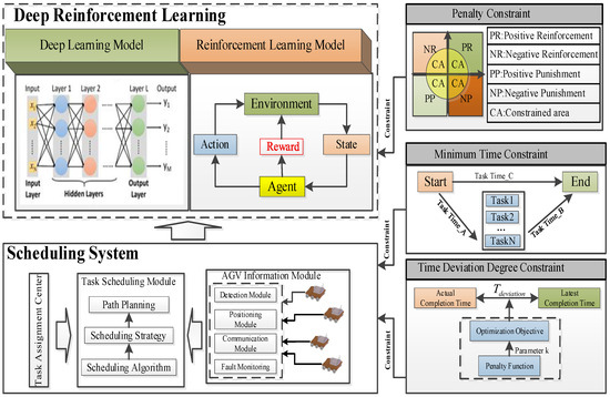
Figure 1. Diagram of Multi-Feature Constraint Relationships.

In logistics scheduling, integrating multi-feature constraints with deep learning algorithms enables the optimization of critical parameters. The deep learning component refines these parameters to generate improved strategies, which act as preference functions for training the reinforcement learning scheduling system. By evaluating response functions, the system assesses whether current actions, states, and rewards directly influence training outcomes. These insights are then incorporated into the reinforcement learning model, where optimized training results are utilized to propose optimal scheduling solutions for the system.

2.2.2. Optimization of the Scheduling System Model

By incorporating a multi-level framework of mutually reinforcing constraints, the enhanced model significantly boosts the scheduling system’s optimization capability. Specifically, the minimum task time constraint ensures balanced resource allocation, thereby mitigating the risk of any AGV becoming an efficiency bottleneck. The minimum scheduling deviation constraint quantitatively integrates business timeliness requirements into the model, prioritizing the completion of critical tasks. Meanwhile, the penalty-based constraint mechanism serves as the foundational implementation framework, translating these constraints, along with physical rules (e.g., collision avoidance) into penalty terms during DRL agent training, thereby ensuring that all decisions remain safe and feasible.

These constraints do not operate independently but form a coordinated closed-loop system that bridges macro-level business objectives with micro-level control instructions. The penalty mechanism guarantees the fundamental feasibility of solutions, while the time and deviation constraints further enhance scheduling quality. Collectively, they guide the system toward a globally optimal solution marked by high efficiency, balanced performance, punctuality, and absolute safety.

The improved scheduling system model is depicted in Figure 2. This model achieves high efficiency and stability by integrating feature constraints into both the control and scheduling layers. By introducing DRL and a multi-constraint optimization mechanism, the enhanced model delivers a qualitative leap in scheduling performance. Its core advantage lies in transitioning from static, rule-driven decision-making to dynamic, intelligent decision-making: the DRL agent possesses real-time perception and response capabilities, enabling flexible adaptation to unexpected events while significantly reducing waiting times and deadlocks. The synergistic multi-constraint mechanism shifts the system’s focus from optimizing single metrics to global multi-objective optimization, encompassing efficiency, balance, and punctuality. This results in substantially improved throughput, reduced task delay rates, and enhanced resource utilization.

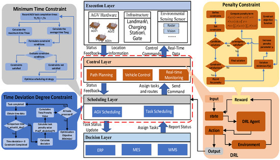
Figure 2. Block Diagram of the Enhanced Multi-Feature Constrained Scheduling Model.

Ultimately, the system exhibits remarkable robustness and adaptability, making it well-suited for complex, highly dynamic environments such as smart warehouses and flexible manufacturing. Thereby, it establishes the essential technological foundation for achieving highly efficient and dependable automated operations.

2.3. Algorithm Design

Numerous DRL algorithms have been developed, and improved versions are continually emerging to overcome inherent limitations. However, their performance is highly dependent on environmental characteristics and parameter configurations. In complex settings like logistics scheduling workshops—characterized by intricate environments, numerous AGVs, tightly coupled task assignments, and stringent operational efficiency requirements—these algorithms often fail to deliver optimal results directly. To address this, this paper introduces an IPPO algorithm. By optimizing scheduling constraint feature parameters, the algorithm enhances its adaptability to complex constraints and multi-objective optimization, thereby significantly improving the training efficiency of the scheduling model and the overall performance of the final scheduling system.

2.3.1. Algorithmic Improvements

(1)

Algorithm Workflow Analysis

As illustrated in Figure 3, the IPPO algorithm operates through a reinforcement learning framework that seamlessly integrates training and deployment within the AGV scheduling system. Based on the standard PPO algorithm, the framework incorporates several key enhancements, including constraint handling, reward design, and training stability. Its core goal is to train a multi-agent scheduling policy that is efficient, stable, and compliant with diverse practical constraints.

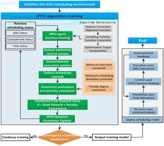
Figure 3. IPPO Algorithm Process Framework Diagram.

The whole process follows a closed-loop paradigm of perception–decision–execution–learning, and can be divided into three main stages:

• Initialization and Environment Construction

The workflow starts with initializing the AGV scheduling environment, including constructing a simulation map, initializing AGV states (e.g., positions, battery levels), and generating initial task queues. This step provides a high-fidelity simulation environment for subsequent training.

2.

Core training loop

This stage forms the heart of the algorithm and follows an iterative optimization process:

State Perception: The IPPO agent perceives the global system state, encompassing the status of all AGVs, environmental information, and task progress, thereby providing comprehensive input for decision-making.

Intelligent Decision-Making: The agent processes the state information through its internal policy network and enhanced optimization modules, ultimately outputting refined control actions such as path selection and velocity commands.

Environment Interaction and Reward Generation: Once actions are executed in the environment, immediate rewards (e.g., task completion rewards) are collected. A constraint evaluation module then computes penalties for violations such as deadline breaches or conflicts. The base rewards and penalties are integrated into a final reward signal.

Learning and Model Update: Using the final reward along with the corresponding state-action data, the algorithm updates the parameters of the policy and value networks, progressively learning improved scheduling strategies. This iterative loop enables the policy to evolve toward optimality.

3.

Convergence Check and Deployment

When the training satisfies the convergence criteria (error below a defined threshold and constraint penalties approaching zero), the iterative loop terminates, and the trained model is exported. The model is then deployed into a practical scheduling system based on a four-layer architecture (decision–scheduling–control–execution), thereby forming a closed-loop intelligent scheduling pipeline from decision-making to execution, ensuring continuous optimization of AGV operations.

In summary, this workflow offers a systematic framework that seamlessly integrates an enhanced reinforcement learning algorithm with complex scheduling challenges, ensuring a smooth transition from simulation-based training to real-world application.

(2)

Analysis of Algorithmic Improvements

The proposed algorithm overcomes the limitations of traditional PPO in complex scheduling scenarios by incorporating several key enhancements, significantly boosting its performance, stability, and practicality.

• The reward signal is explicitly decomposed into two components: a “base reward” and a “dynamic penalty term”. The penalty term is calculated by a dedicated constraint evaluation module and weighted using a penalty-degree function.

Benefits: Clearer optimization objectives: The agent can better distinguish between rewarded behaviors (e.g., task completion) and penalized behaviors (e.g., constraint violations), thereby improving learning efficiency.

Mitigation of reward sparsity: Constraint penalties provide denser feedback signals, helping the agent avoid invalid or hazardous behaviors during early exploration and improving learning performance in traditionally sparse reward environments.

2.

Building upon PPO’s clipping mechanism, a sampling bias correction technique is introduced to minimize deviations during off-policy learning.

Benefits: Enhanced training stability: By reducing variance during policy updates, training stability is improved, and the risk of training collapse is minimized.

Improved sample efficiency: Historical sample data can be utilized more effectively, enabling more rounds of meaningful learning with the same amount of data and thereby accelerating convergence.

3.

Agent decisions are based on the global system state rather than the local observations of individual AGVs.

Benefits: Enhanced collaborative decision-making: By perceiving the states and intentions of other AGVs, agents can coordinate their actions, effectively reducing path conflicts and resource contention.

Achievement of system-level optimization: The decision-making objective shifts from optimizing the efficiency of individual AGVs to improving overall system performance, such as total task completion time and other global metrics.

2.3.2. Optimization Strategies and Parameter Improvements

The optimization strategy refines parameters of the scheduling system model, employing an optimization function to conduct computations in multi-feature constrained environments. Aligning with feature-specific objectives ensures efficient operation of the scheduling system. This strategy primarily targets optimization across three domains: policy gradients, policy networks, and objective networks. This approach facilitates the analysis of reward values, thereby enhancing the AGV’s adaptability to the scheduling environment and progressively improving the operational efficiency of the scheduling system.

(1)

Objective Function with Feature Constraints

In reinforcement learning, an objective function is introduced to leverage the interaction between actions, states, and the scheduling environment to obtain corresponding reward values. This process adjusts model parameters to minimize the error between predicted and actual result values, thereby updating the results. Finally, according to the gradient strategy, the desired expected value is achieved to facilitate the operational update process, and the expression for the objective function is presented in Equation (8):

$$\mathit{CE}\left(\widehat{y}\right)=-{\displaystyle \frac{1}{n}}{\displaystyle \sum _{z=1}^n\left[I\left\{y=y^{\prime }\right\}\log \left(p_t\right)\right]}$$

(8)

Equation (8) incorporates the number of samples collected for training items n, the actual calibration value y, the desired output value y’, the probability value of the actual event distribution p_t, and the estimated probability value of the task occurrence predicted by the AGV. This objective function enables iterative calculation of training sample data. However, practical operations may encounter large estimation variances, necessitating the use of the AC framework for estimation. This framework provides feedback on the expected gain of the current state after action execution, thereby facilitating the utilization of sample data.

Under feature constraints, constraint parameters are introduced to adjust the objective function, enabling the training model to perform goal-directed analysis and producing the estimated probability value, as expressed in Equation (9):

$$p_{\prime }^t={\displaystyle \frac{{\displaystyle \sum _m^M{Q}_m}\min \left\{{\overline{T}}_{mc}\left(k\right)\right\}-{\displaystyle \sum _n^{N_s}{\displaystyle \sum _m^M{\displaystyle \sum _c^C\left(\left|{\underset{after}{T}}_{mc}^D-{\underset{befor}{T}}_{mc}^D\right|\right)}}}}{{\displaystyle \sum _m^M{Q}_m}\min \left\{{\overline{T}}_{mc}\left(k\right)\right\}}}$$

(9)

Substituting Equation (9) into Equation (8) yields the optimized objective function, as shown in Equation (10):

$$\Psi \left(\widehat{y}\right)=-{\displaystyle \frac{1}{n}}{\displaystyle \sum _{z=1}^n\left[I\left\{y=y^{\prime }\right\}\log \left(p_{\prime }^t\right)\right]}$$

(10)

(2)

Sampling Correction Function

The IPPO algorithm employs a sampling correction function to perform unbiased estimation operations on the expected value of the optimization objective function. Initially, a feedback training sample dataset is utilized to control the variance of calculation results in accordance with the feature distribution of the optimization strategy, ensuring accurate estimation of the estimated variance by introducing a correction function into the objective function. Equation (11) presents the correction function incorporated into the objective function:

$$E\left(\kappa \right)=E_{s~\pi }\left[{\displaystyle \frac{{\pi }_{\kappa }\left(s,a\right)}{{\pi }_{{\kappa }^{\prime }}\left(s^{\prime },a^{\prime }\right)}}\left(Q_{{\kappa }^{\prime }}\left(s^{\prime },a^{\prime }\right)-V_{{\kappa }^{\prime }}\left(s^{\prime }\right)\right)\right]$$

(11)

where ${\pi }_{\kappa }$ denotes the optimal policy function for AGV-scheduling environment interaction, ${\pi }_{{\kappa }^{\prime }}$ represents the policy for sampling environmental interactions, $s$ and $a$ express the trained state and action values, respectively, $s^{\prime }$ and $a^{\prime }$ denote the trained desired state and action values, respectively, $V_{\kappa }\left(s\right)$ represents the state value function, and $Q_{\kappa }$ denotes the desired state function value.

(3)

Optimization Objectives

The sample data generated from AGV-scheduling environment interactions exhibit a large variance in distribution estimation, leading to significant errors in target values. Therefore, target value optimization is essential. This optimization is achieved by introducing an importance weight function, which is substituted into Equation (11) to obtain the optimized target function, as shown in Equation (12):

$$E^{\prime }\left(\kappa \right)=E_{s~\pi }\left[\min \left(r_t\left(\kappa \right),clip\left(r_t\left(\kappa \right),1-\epsilon ,1+\epsilon \right)\right)\right] \left(Q_{{\kappa }^{\prime }}\left(s^{\prime },a^{\prime }\right)-V_{{\kappa }^{\prime }}\left(s^{\prime }\right)\right)$$

(12)

Using the optimization function, it is known that the importance weight $r_t\left(\kappa \right)$ is restricted between $\left[1-\epsilon ,1+\epsilon \right]$ ranges, where $\epsilon$ denotes the hyperparameters. Moreover, adjusting the parameters allows for the modification of weight values.

2.3.3. Algorithm Pseudocode

To cope with the challenges of low efficiency and high dynamism in AGV scheduling systems, this study introduces an IPPO algorithm. The innovation lies in the seamless integration of constrained optimization with reinforcement learning. By incorporating a penalty-based constraint mechanism for dynamically manage hard constraints and a multi-stage optimization module, the algorithm guarantees that the scheduling policy not only maximizes system performance but also adheres to all operational constraints.

Traditional approaches typically embed constraints into the reward function using fixed penalty coefficients, which makes it challenging to achieve a balance between constraint satisfaction and performance optimization, frequently resulting in unstable training or the generation of infeasible policies. The enhanced algorithm proposed in this study tackles these issues through three pivotal modules:

Action Improvement Module: This module directly incorporates scheduling constraints into the objective function via Lagrange multipliers, steering the policy towards the feasible domain from the outset.

Dynamic Penalty Mechanism: By employing an adaptively penalized constraint function, our approach mitigates the over-suppression of early exploration and the oversight of late-stage constraints, leading to significantly improved convergence and more feasible solutions.

Constraint-Aware Policy Update: This mechanism integrates the degree of constraint violation into the policy gradient update, facilitating the collaborative optimization of both performance and constraint satisfaction.

Consequently, the algorithm is capable of generating scheduling policies that are both highly efficient and robustly reliable, striking an optimal balance between computational performance and system stability. These policiesenable seamless integration into the practical four-layer “Decision-Scheduling-Control-Execution” architecture, ensuring effortless interoperability across various operational levels. For enhanced clarity and reproducibility, Algorithm 1 systematically delineates the IPPO scheduling workflow, detailing the iterative interplay between agents and environments. Algorithm 2 further elaborates on the action optimization model, which refines candidate actions through multi-objective evaluation and feasibility assessments. Finally, Algorithm 3 provides a comprehensive description of the constraint-aware policy update mechanism, incorporating safety boundaries and operational limits into the learning process to enforce policy compliance with real-world demands.

Algorithm 1 IPPO for AGV Scheduling

$\begin{array}{l}Input:Environment env:AGV scheduling simulation environment\\ IPPOAgent agent:RL agent with policy and value networks \\ Hyperparameters:MAX\_EPISODES,CONSTRAINT\_TOLERANCE,\\ \lambda (Lagr angian multipliers),\\ \mu (penalty coefficients)\\ Output:Trained policy network \pi \_\theta ,Value network V\_\varphi \\ Phase 1: Initialization\\ Initialize:env \leftarrow AGV Environment(map\_file,AGV\_config,task\_queue)\\ agent \leftarrow IPPO Agent(state\_dim,action\_dim)\\ \lambda ,\mu \leftarrow initial\_lagrangian\_parameters()\\ Phase 2: Training Cycle\\ for episode=1 to MAX\_EPISODES do:\\ state \leftarrow env.reset()\\ episode\_reward \leftarrow 0\\ while not env.terminated() do:\\ Action Selection and Execution\\ action \leftarrow agent.policy\_network(state)\\ action\_optimized \leftarrow agent.improve\_action(state,action) \left(Algorithm 2\right)\\ next\_state,immediate\_reward,done \leftarrow env.step(action\_optimized)\\ Constraint-Aware Reward Computation\\ constraint\_violation \leftarrow compute\_constraint\_violation(state,action\_optimized,next\_state)\\ penalty \leftarrow \lambda ·constraint\_violation+(\mu /2)·constraint\_violation²\\ \left(Augmented Lagrangian\right)total\_reward \leftarrow immediate\_reward-penalty\\ Store transitionagent.buffer.store(state,action,total\_reward,next\_state,done)\\ state \leftarrow next\_state\\ episode\_reward \leftarrow episode\_reward+total\_reward\\ Constraint-Aware Policy Update\\ if agent.update\_condition() then:\\ advantages \leftarrow agent.compute\_advantages()\\ agent.update\_policy(advantages,constraint\_violation) \left(Algorithm 3\right)\\ Update Lagrangian parameters\lambda \leftarrow \lambda +\mu ·constraint\_violation\\ \mu \leftarrow min(\mu \_max,\mu ·scale\_factor)\\ Convergence Check\\ if agent.has\_converged()andmax(constraint\_violation)<CONSTRAINT\_TOLERANCE:\\ break\\ Phase 3: System Deployment\\ deployment\_system \leftarrow Scheduling System(agent.policy\_network)\\ deployment\_system.run()\end{array}$

Algorithm 2 Action Improvement Module (Improve_Action)

$\begin{array}{l}Input:state s,initial action a \\ Output:Optimized action a\_optimized Procedure improve\_action(s,a):\\ Feature-constrained objective\\ a\_constrained \leftarrow argmin\_a[L(s,a)+\Sigma \_i \lambda \_i·c\_i(s,a)]\\ Correction of sampling bias\\ a\_corrected \leftarrow a\_constrained-\beta ·\nabla D\_KL(\pi \_old||\pi \_new)\\ Final optimization\\ a\_optimized \leftarrow argmin\_a[J(\pi \_\theta )+\alpha ·H(\pi \_\theta )]\\ returna\_optimized\end{array}$

Algorithm 3 Constraint-Aware Policy Update (Update_Policy)

$\begin{array}{l}Input:Advantages A,constraint violations C \\ Output:Updated policy parameters \theta Procedure update\_policy(A,C):\\ Compute policy gradient with constraint awareness\\ policy\_loss \leftarrow -E[min(r(\theta )·A,clip(r(\theta ),1-\epsilon ,1+\epsilon )·A)]\\ constraint\_loss \leftarrow \Sigma \_i \lambda \_i·c\_i(s,a)\\ Combined loss function\\ total\_loss \leftarrow policy\_loss+constraint\_loss+value\_loss\\ Gradient descent\theta \leftarrow \theta -\eta \_\theta ·\nabla \_\theta total\_loss\\ \varphi \leftarrow \varphi -\eta \_\varphi ·\nabla \_\varphi value\_loss\\ return\theta ,\varphi \end{array}$

In the IPPO algorithm, $\pi \_\theta$ denotes the policy network parameterized by $\theta$, responsible for generating action decisions, while $V\_\varphi$ represents the value network parameterized by $\varphi$, used for state-value estimation. $L\left(s,a\right)$ is the task completion time objective function, measuring scheduling performance, and $c\_i\left(s,a\right)$ denotes the i-th constraint function (e.g., time window constraints, collision avoidance), representing hard conditions that the system must satisfy. $\lambda$ and $\mu$ are the multiplier vector and penalty coefficient in the augmented Lagrangian method, respectively, used to transform the constrained optimization problem into an unconstrained form. $r\left(\theta \right)$ represents the probability ratio in policy updates, i.e., the ratio between $\pi \_\theta \left(a\left|s\right.\right)$ and the old policy $\pi \_\theta \_old\left(a\left|s\right.\right)$, which is a core concept in Proximal Policy Optimization. $H\left(\pi \_\theta \right)$ denotes the policy entropy, used to encourage exploration and prevent the policy from prematurely converging to local optima.

3. Experimental Design

3.1. Experimental Dataset

The dataset employed in this experiment is predominantly derived from multimodal operational data generated during AGV transport scheduling tasks, including action data, state data, and optimization feature constraint data, which collectively form the training samples for analyzing the interactive dynamics between AGVs and the scheduling environment. To meet scheduling demands under multiple constraints, the system adopts a DRL-based scheduling model, utilizing the IPPO algorithm to bolster both training stability and scheduling performance. The model integrates various feature constraint parameters—such as minimum task completion time, penalty coefficients, and time deviation—into the IPPO objective for joint optimization.

Specifically, the action data encompass variables like the velocity, travel distance, steering angle, and task execution status of multiple AGVs. The state data include AGV positional information, task status, and path topology. The optimization feature constraint data are utilized to assess the disparity between algorithm-predicted values and actual operational results, serving as feedback parameters to refine action decisions and thereby enhance model accuracy and generalization capabilities. All data are collected in real-time, and the scheduling dataset is generated through simulation experiments. This dataset facilitates quantitative comparison and analysis of different algorithmic strategies, validating the practical efficacy of the proposed algorithm in enhancing scheduling efficiency.

3.2. Simulation Platform Setup

Simulation experiments for the scheduling system model are conducted using the specialized simulation platform, ProfControlV8 (Figure 4a,b), which emulates system operational states during the training. Prior to simulation, initial parameters’ basic simulator settings and operational states are configured to create a scheduling environment that closely mirrors real-world conditions. The simulation process is segmented into three primary stages according to the task workflow: reception, waiting, and execution. Functional operational data are gathered at each stage to evaluate the overall scheduling efficiency.

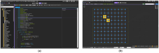
Figure 4. Simulation Environment Setup in the Simulator. (a) Program Script Development Interface. (b) AGV Scheduling Simulation Interface.

During the task execution phase of the simulation, multiple AGVs are modeled operating within a logistics workshop setting. The system dynamically selects the most suitable AGV for each task, taking into account the interplay between task volume and AGV availability (e.g., scenarios where task numbers surpassed or fell short of AGV numbers). This selection process leverages optimized feature constraint parameters derived from the training model, including task completion time, reward–penalty coefficients, and time deviations.

In the task waiting phase, the simulation replicated scenarios where the number of AGVs exceeded task requirements or fell within a predefined range. This phase encompassed AGVs idling as they awaited new tasks and transitioning to a standby state upon task completion.

The task reception stage primarily focused on simulating the decision-making and allocation process following an AGV’s task acquisition, with the objective of achieving optimal task distribution. When constructing the logistics workshop simulation environment, crucial parameters such as spatial layout, AGV quantity, task volume, and task execution sequence were meticulously defined.

3.3. Model Parameter Settings

The scheduling system was simulated using a dedicated simulator, with the scheduling model framework applied to enhance DRL training. Given the multi-constraint nature of the scheduling model, the deep neural network model facilitates the optimization of these feature parameters. However, to ensure the realism of the training process during simulation, it was imperative to define relevant operational parameters. Therefore, the training-related parameters of the scheduling system model are meticulously configured to rigorously validate the scheduling model’s effectiveness. In this experiment, parameter settings were categorized into three parts: reward function parameters, IPPO algorithm hyperparameters, and model training configuration parameters.

3.3.1. Reward Function Parameter Settings

The model’s reward function is structured around a blend of sparse rewards and dense penalties, with parameter settings outlined in Table 1. The central premise is to offer a substantial positive reward (+100) to distinctly encourage task completion as the primary objective, supplemented by a modest per-step time-saving reward (+1/step) to refine efficiency optimization. To ensure both safety and efficiency, a significant collision penalty (−500) and a minor waiting penalty for idle time (−0.1/step) are incorporated. These rewards and penalties collectively steer the agent towards prioritizing safety while mastering the swift and efficient completion of scheduling tasks.

Table 1. Reward Function Parameter Settings.

Parameter	Value
Base Reward Events and Values	+100 (for completing the task), +1 (for saving time at each step)
Collision Penalty Value	−500
Awaiting Punishment (At Every Turn)	−0.1
Repeated Updates	5
Clipping Factor	0.1

3.3.2. IPPO Algorithm Hyperparameter Settings

The algorithm hyperparameters were carefully tuned in accordance with the PPO methodology, which emphasizes stability and sustained performance over time, with settings summarized in Table 2.

Table 2. Learning Hyperparameter Settings.

Parameter	Value
Learning Rate	0.0003
PPO Clipping Range (ε)	0.2
Discount Factor	0.99
GAE (λ) Coefficient	0.95
Entropy Reward Coefficient	0.01
Value Loss Coefficient	0.5

A learning rate of 3 × 10⁻⁴ was adopted as a standard setting to achieve an optimal balance between convergence speed and training stability, while the clipping range was set at 0.2, serving as a critical safeguard against overly aggressive policy updates. A high discount factor of 0.99, coupled with a GAE coefficient of 0.95, indicates the model’s strong focus on long-term returns, guiding it to develop forward-looking scheduling strategies. Additionally, an entropy coefficient of 0.01 was introduced to sustain sufficient exploration, while a value loss coefficient of 0.5 was employed to ensure the stability of value network training.

3.3.3. Model Training Configuration Parameters

The training configuration embodies a modern DRL paradigm that prioritizes parallelization, large batch processing, and extensive training, with parameter configurations summarized in Table 3. By deploying 8 parallel environments, a rich diversity of data was efficiently gathered. Each update drew upon 10,000 steps of experience, distributed across 5 mini-batches and iterated 5 times, maximizing the utilization of sample data. The training process concluded after a cumulative total of one million interactions across all environments, affording the agent ample opportunities to learn complex scheduling strategies and resulting in a mature, reliable model.

Table 3. Model Training Parameter Settings.

Parameter	Value
Number of Independent Agents	0.001
Number of Parallel Training Environments	0.99
Steps Collected per Update	10,000
Batch Size per Update	5
Number of Iterations per Update	0.1
Total Training Time Steps	0.000006
Total Number of Training Tasks	50

4. Results and Discussion

4.1. Variation in Constraint Values Under Feature Conditions

As the number of iterations of the IPPO algorithm continued to increase, the comprehensive performance of the AGV scheduling model under multiple constraints demonstrated systematic improvement. As shown in Table 4, throughout ten thousand iterations, three key performance indicators—minimum task completion time (Ts), penalty term (P), and scheduling time deviation (H)—all exhibited a steady declining trend: the task completion time improved from 98.2 s to 30 s, the penalty term decreased from 130 to 82, and the time deviation significantly converged from 12 s to just 0.5 s. Table 5’s statistical analysis reveals the relationship between these metrics and constraint conditions. All indicators stabilized at low levels: task completion time variation coefficient reached 3.6%, penalty term maintained at 82.5 ± 3.2, and time deviation converged to 0.52 s despite its 28.8% variation coefficient. With significant statistical differences (p < 0.005) and large effect sizes (Cohen’s d > 1.5), these results confirm IPPO’s effectiveness in achieving substantial scheduling improvement while satisfying complex constraints.

Table 4. Variation in Feature Parameters under Constraints.

Number of Iterations	Minimum Task Completion Time (s)	Penalty (P)	Scheduling Time Deviation (s)
1000	98.2	130	12
2000	75	120	9.5
3000	60	110	7.5
4000	50	105	5.8
5000	42	98	4.2
6000	37	94	3.2
7000	34	91	2.4
8000	32	89	1.6
9000	31	85	1.0
10,000	30	82	0.5

Table 5. Statistical Analysis Results of Performance Metrics.

Performance Metric	Final Result (Mean ± SD)	95% Confidence Interval	Coefficient of Variation	Statistical Significance (p-Value)	Effect Size (Cohen’s d)
Minimum Task Completion Time (s)	30.2 ± 1.1	[29.8, 30.6]	3.6%	p < 0.001	2.1 (Large Effect)
Penalty (P)	82.5 ± 3.2	[80.6, 84.4]	3.9%	p < 0.005	1.8 (Large Effect)
Scheduling Time Deviation (s)	0.52 ± 0.15	[0.42, 0.62]	28.8%	p < 0.001	1.5 (Large Effect)

Based on the convergence data from Table 4 and Figure 5, the minimum task completion time (Ts) plummeted from 98.2 s to 30 s, marking a reduction of 68.2 s (a 69.4% improvement). During the initial iterations (1000–3000), the optimization process proceeded at a rapid pace, with a decrease of 38.2 s, reflecting the model’s swift assimilation of scheduling strategies. In the subsequent middle to later iterations (3000–10,000), the rate of optimization slowed, yet it still achieved a reduction of 30 s, indicating the model’s transition into a fine-tuning phase. The penalty (P), acting as a constraint indicator, decreased from 130 to 82 (a 37% reduction) with a smooth curve, showing that the constraint mechanism effectively guided policy optimization and improved in synchrony with Ts and H, demonstrating a coordinated enhancement of efficiency and constraint satisfaction. The time deviation (H) dropped from 12 s to 0.5 s (a 95.8% reduction), signaling a substantial decrease in policy fluctuations and a convergence towards stable scheduling outcomes. The exceptionally low deviation underscores the system’s high reliability, validating the improved IPPO algorithm’s capacity to generate robust scheduling strategies in complex, dynamic environments.

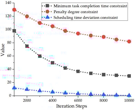
Figure 5. Variation in Constraint-Related Feature Parameters.

Analyzing the relative interplay among feature constraints, as depicted in Figure 6a,b, reveals that the fitted relationships between P and Ts, as well as H and Ts, are approximately linear. This underscores Ts as the pivotal driver of system performance, with P and H acting as constraint feedback indicators that are closely intertwined with Ts. Together, they comprehensively depict the progression of scheduling performance enhancement. Strong positive correlations were identified between Ts and P, Ts and H, and P and H, with correlation coefficients hovering around 0.99, 0.98, and 0.97, respectively. This indicates that the reduction in task completion time does not come at the cost of breaching constraints; instead, it is achieved in tandem with the concurrent optimization of penalty and time deviation, enabling the algorithm to attain simultaneous improvements in efficiency and constraint adherence, validating its efficacy in balancing performance objectives.

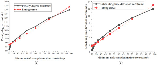
Figure 6. Correlation Analysis among Feature Constraints. (a) Correlation between Penalty and Minimum Task Completion Time Constraint. (b) Correlation between Scheduling Time Deviation and Minimum Task Completion Time Constraint.

4.2. Comparative Analysis of Task Completion Timeliness in the Scheduling System

To scientifically assess the performance of the proposed IPPO algorithm, a rigorous experimental comparison framework is devised. The central premise of the experiment was to select representative scheduling algorithms and conduct an impartial comparison within an identical simulation environment, including uniform map layouts, AGV quantities, and task sequences, thereby eliminating external confounding factors. The algorithms under comparison included: a baseline rule-based scheduling algorithm (utilizing a “shortest-distance-first” allocation strategy and “A* path planning”), a GA emblematic of traditional optimization techniques, and the proposed DRL-based IPPO algorithm. The primary performance metric was task completion time, analyzed from three dimensions: individual task completion times, the distribution of completion times across all tasks, and the system-wide makespan, aiming to provide a comprehensive and objective evaluation of each algorithm’s efficiency and performance.

4.2.1. Validation of Individual Task Completion Time

As illustrated in Figure 7a–c, the comparison of individual task completion times reveals that, after 10,000 iterations of training, the IPPO algorithm substantially reduced the average completion time per task from 68 s to 30 s, achieving a 55.9% performance enhancement—significantly outpacing the 11.8% improvement of the GA and the 3.2% improvement of the rule-based scheduling. Performance benchmarks indicate that the IPPO algorithm is 2.5 times faster than the GA and 3.1 times faster than the rule-based method, underscoring a distinct efficiency advantage.

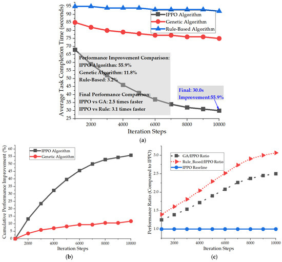
Figure 7. Variation of Individual Task Completion Time. (a) Single Task Average Completion Time vs. Iteration Steps. (b) Algorithm Performance Improvement Speed Comparison. (c) Performance Ratio Comparison: Other Algorithms vs. IPPO.

The learning curve exhibits hallmark characteristics of reinforcement learning: rapid learning (0–3000 iterations) yielding a 23.5% improvement, intermediate fine-tuning (3000–7000 iterations) achieving a 34.6% enhancement, and stable convergence in the later stages (after 7000 iterations), with performance fluctuations of merely ±2.1 s, demonstrating exceptional convergence and stability. Specifically, after 10,000 iterations, IPPO achieved a 55.9% reduction in average task completion time (decreasing from 68 s to 30 s), whereas GA achieved only an 11.8% reduction. The efficiency ratio is calculated as (55.9%/10,000 iterations) ÷ (11.8%/10,000 iterations) ≈ 4.7, demonstrating that IPPO improves performance 4.7 times faster per iteration than GA.

4.2.2. Validation of Completion Time for All Tasks

Based on the simulation results depicted in Figure 8a–d, the IPPO algorithm showcased exceptional performance across all task scheduling scenarios. After 10,000 iterations, it slashed the average task completion time from 98.2 s to 32.5 s, marking a 66.9% improvement that substantially surpassed the GA’s 45.2% and the rule-based scheduling’s 8.1%. The standard deviation of task completion times under IPPO also dropped from 25.3 s to 8.7 s, reflecting the highest level of scheduling stability among other algorithms. The performance improvement factor soared to 2.96, far outstripping those of the competing algorithms.

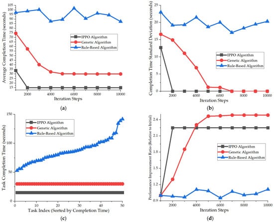
Figure 8. Analysis of Completion Time Curves for All Tasks. (a) Average Completion Time Trend. (b) Completion Time Standard Deviation Trend (Stability Analysis). (c) All Tasks Completion Time Distribution at Final Iteration. (d) Performance Improvement Ratio Comparison.

During the rapid learning phase (0–3000 iterations), IPPO attained a 40% performance enhancement and sustained stable convergence in the later stage. These results demonstrate the algorithm’s highly efficient learning capability, outstanding optimization prowess, and strong stability in multi-task scheduling environments, significantly boosting overall system throughput and scheduling efficiency.

4.2.3. Validation of System Makespan

Optimization efficiency is defined as performance improvement percentage per iteration, calculated by dividing the makespan reduction rate by the required convergence iterations. This metric balances solution quality and computational cost for fair algorithm comparison. The IPPO algorithm exhibited decisive performance superiority in optimizing the scheduling system’s total makespan. As illustrated in Figure 9a–d, the final makespan reached just 85.2 s, achieving speeds 2.14 times and 3.47 times faster than the GA and rule-based scheduling, respectively, with a substantial performance improvement of 61.5%. The algorithm exhibited strong convergence characteristics, essentially stabilizing after 5000 iterations, with 90% of its performance gains achieved by the 4000-iteration mark. After convergence, fluctuations remained minimal (±3.2 s), indicating excellent stability and learning efficiency. The IPPO algorithm efficiently streamlined the process from 221.5 s to 85.2 s through three well-defined phases: rapid learning, fine-tuning, and stable convergence.

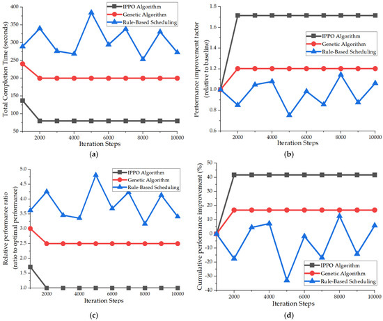
Figure 9. Analysis of Total Makespan Variation in the Scheduling System. (a) Trend in Total Completion Time with Iteration Count. (b) Overall Completion Time Performance Improvement Factor. (c) Relative Performance Comparison. (d) Convergence Rate Analysis.

As depicted in Figure 9a–d, the IPPO algorithm delivered outstanding overall performance, averaging a 12.3% improvement per 1000 iterations and attaining an optimization efficiency 2.7 times greater than that of the GA. This demonstrates its high learning capacity and efficient resource utilization. In practical applications, compared to rule-based scheduling, it slashed operational time by 210.4 s, enhancing efficiency by 347%. By enabling intelligent scheduling, the algorithm markedly reduces equipment idle time, boosts system throughput, and demonstrates strong robustness and scalability, offering an efficient and reliable technical solution for optimizing intelligent manufacturing and logistics systems.

4.3. Research Limitations

This study primarily exhibits limitations in four aspects: the experimental environment is based on a simulation platform, resulting in discrepancies with real-world scenarios; the algorithm’s performance in ultra-large-scale AGV clusters remains unverified; the training phase requires substantial computational resources with convergence speed needing improvement; practical applications also face challenges in specialized parameter tuning and system integration compatibility. These limitations provide clear directions for future research improvements.

5. Conclusions

This study introduces a multi-AGV task scheduling approach based on multi-feature constraints and an enhanced DRL framework (IPPO). By integrating constraints such as minimum task completion time, penalty, and scheduling time deviation, the method effectively integrates constrained optimization with DRL. To overcome the inefficiencies of sluggish convergence and limited stability inherent in traditional scheduling methods within complex environments, the IPPO algorithm underwent several refinements: a dynamic penalty mechanism, a structured reward function, sample correction, and global state awareness, achieving dual optimization of scheduling efficiency and constraint satisfaction.

Simulation results reveal that after 10,000 iterations, the minimum task completion time plummeted from 98.2 s to 30 s (a 69.4% improvement), penalties decreased from 130 to 82 (a 37% reduction), and scheduling time deviation shrunk from 12 s to 0.5 s (a 95.8% reduction).

In comparison with other algorithms, the IPPO algorithm accomplished individual task completion times 2.5 times faster than the GA and 3.1 times faster than rule-based scheduling. The system’s makespan is reduced by 61.5%, with convergence and stability outpacing alternative methods.

The optimization process mirrored classic reinforcement learning traits: swift learning in the initial phase, fine-tuning in the middle stage, and stable convergence in the later stage, with negligible performance fluctuations.

In conclusion, the refined IPPO algorithm has been validated to achieve efficient scheduling, stable convergence, and multi-constraint cooperative optimization in intricate dynamic settings, substantially boosting the throughput and reliability of multi-AGV systems. This approach offers a practical, scalable solution for large-scale task scheduling in intelligent manufacturing and smart logistics, holding significant promise for real-world application and broader industry adoption.

References

- Gianfrancesco, M.A.; Tamang, S.; Yazdany, J.; Schmajuk, G. Potential biases in machine learning algorithms using electronic health record data. JAMA Intern. Med. 2018, 178, 1544–1547. [Google Scholar] [CrossRef]
- Lan, Y.L.; Liu, F.; Ng, W.W.; Zhang, J.; Gui, M. Decomposition-based multi-objective variable neighborhood descent algorithm for logistics dispatching. IEEE Trans. Emerg. Top. Comput. Intell. 2020, 5, 826–839. [Google Scholar] [CrossRef]
- Kruger, K.; Basson, A. Erlang-based holonic controller for a palletized conveyor material handling system. Comput. Ind. 2018, 101, 1–12. [Google Scholar] [CrossRef]
- Forger, G. AGVs set new standards for inventory transportation. Mod. Mater. Handl. 2022, 77, 40–50. [Google Scholar]
- Zhou, L.; Zhang, L.; Fang, Y. Logistics services scheduling with manufacturing provider selection in cloud manufacturing. Robot. Comput.-Integr. Manuf. 2020, 65, 101914. [Google Scholar] [CrossRef]
- Wang, X.; Wu, W.; Xing, Z.; Chen, X.; Zhang, T.; Niu, H. A neural network-based multi-state scheduling algorithm for multi-AGV system in FMS. J. Manuf. Syst. 2022, 64, 344–355. [Google Scholar] [CrossRef]
- Boccia, M.; Masone, A.; Sterle, C.; Murino, T. The parallel AGV scheduling problem with battery constraints: A new formulation and a matheuristic approach. Eur. J. Oper. Res. 2023, 307, 590–603. [Google Scholar] [CrossRef]
- Popper, J.; Yfantis, V.; Ruskowski, M. Simultaneous production and AGV scheduling using multi-agent deep reinforcement learning. Procedia CIRP 2021, 104, 1523–1528. [Google Scholar] [CrossRef]
- Bohács, G.; Gyrváry, Z.; Gáspár, D. Integrating scheduling and energy efficiency aspects in production logistics using AGV systems. IFAC-Pap. 2021, 54, 294–299. [Google Scholar] [CrossRef]
- Yuan, M.H.; Li, Y.D.; Pei, F.Q.; Gu, W.B. Dual-resource integrated scheduling method of AGV and machine in intelligent manufacturing job shop. J. Cent. South Univ. 2021, 28, 2423–2435. [Google Scholar] [CrossRef]
- Du, H.; Jiang, X.; Lv, M.; Yang, T.; Wang, Y. Scheduling and analysis of real-time task graph models with nested locks. J. Syst. Archit. 2020, 114, 101969. [Google Scholar] [CrossRef]
- Atik, M.E.; Duran, Z.; Seker, D.Z. Machine learning-based supervised classification of point clouds using multiscale geometric features. ISPRS Int. J. Geo-Inf. 2021, 10, 187. [Google Scholar] [CrossRef]
- Liang, H.; Seo, S. Lightweight deep learning for road environment recognition. Appl. Sci. 2022, 12, 3168. [Google Scholar] [CrossRef]
- Weon, I.-S.; Lee, S.-G. Environment recognition based on multi-sensor fusion for autonomous driving vehicles. J. Inst. Control. Robot. Syst. 2019, 25, 65599–65608. [Google Scholar] [CrossRef]
- Wang, L.; Li, R.; Shi, H.; Sun, J.; Zhao, L.; Seah, H.; Quah, C.; Budianto, T. Multi-channel convolutional neural network-based 3D object detection for indoor robot environmental perception. Sensors 2019, 19, 893. [Google Scholar] [CrossRef] [PubMed]
- Zhang, T.; Lam, K.-Y.; Zhao, J. Deep reinforcement learning-based scheduling strategy for federated learning in sensor-cloud systems. Future Gener. Comput. Syst. 2023, 144, 219–229. [Google Scholar] [CrossRef]
- Wang, S.; Li, Y.; Pang, S.; Lu, Q.; Wang, S.; Zhao, J. A task scheduling strategy in edge-cloud collaborative scenario based on deadline. Sci. Program. 2020, 2020, 3967847. [Google Scholar] [CrossRef]
- Guo, Q. An optimal scheduling path algorithm for enterprise resource allocation based on workflow. J. Eur. Des. Systèmes Autom. 2020, 53, 1–12. [Google Scholar] [CrossRef]
- Zhang, L.; Hu, Y.; Wang, C.; Tang, Q.; Li, X. Effective dispatching rules mining based on near-optimal schedules in intelligent job shop environment. J. Manuf. Syst. 2022, 63, 424–438. [Google Scholar] [CrossRef]
- Yang, S.; Wang, J.; Xu, Z. Real-time scheduling for distributed permutation flowshops with dynamic job arrivals using deep reinforcement learning. Adv. Eng. Inform. 2022, 54, 101776. [Google Scholar] [CrossRef]
- Huo, Z.; Zhu, W.; Pei, P. Network traffic statistics method for resource-constrained industrial project group scheduling under big data. Wirel. Commun. Mob. Comput. 2021, 2021, 5594663. [Google Scholar] [CrossRef]
- Ramos, A.S.; Miranda Gonzalez, P.A.; Nucamendi Guillén, S.; Olivares Benitez, E. A formulation for the stochastic multi-mode resource-constrained project scheduling problem solved with a multi-start iterated local search metaheuristic. Mathematics 2023, 11, 337. [Google Scholar] [CrossRef]
- Schäffer, L.E.; Helseth, A.; Korpås, M. A stochastic dynamic programming model for hydropower scheduling with state-dependent maximum discharge constraints. Renew. Energy 2022, 194, 571–581. [Google Scholar] [CrossRef]
- Smutnicki, C.; Pempera, J.; Bocewicz, G.; Banaszak, Z. Cyclic flow-shop scheduling with no-wait constraints and missing operations. Eur. J. Oper. Res. 2022, 302, 39–49. [Google Scholar] [CrossRef]
- Yang, S.; Xu, Z. Intelligent scheduling and reconfiguration via deep reinforcement learning in smart manufacturing. Int. J. Prod. Res. 2022, 60, 243–252. [Google Scholar] [CrossRef]
- Chawla, V.K.; Chanda, A.K.; Angra, S. Simultaneous dispatching and scheduling of multi-load AGVs in FMS: A simulation study. Mater. Today Proc. 2018, 5, 25358–25367. [Google Scholar] [CrossRef]
Disclaimer/Publisher’s Note: The statements, opinions and data contained in all publications are solely those of the individual author(s) and contributor(s) and not of MDPI and/or the editor(s). MDPI and/or the editor(s) disclaim responsibility for any injury to people or property resulting from any ideas, methods, instructions or products referred to in the content. |
© 2025 by the authors. Licensee MDPI, Basel, Switzerland. This article is an open access article distributed under the terms and conditions of the Creative Commons Attribution (CC BY) license (https://creativecommons.org/licenses/by/4.0/).