Impact of Partitioning Methods on the Accuracy of Coarse-Grid Network Reservoir Models

Abstract

Reservoir simulation remains a major computational bottleneck for production optimization, history matching, and uncertainty quantification, particularly as geological models become increasingly detailed and recovery processes more complex. Coarse-grid network (CGNet) models have recently emerged as an efficient, physics-grounded proxy to full-physics simulations by solving the flow equations on a coarse network whose parameters are freely calibrated to reproduce fine-scale or observed well responses. In this study, we investigate how different coarse-partitioning strategies affect the accuracy and robustness of CGNet models. Four partitioning approaches are examined: a simple cookie-cutter partition, and three partitions based on cell-wise indicators—absolute permeability, velocity magnitude, and the product of forward and backward time-of-flight. Two test cases are considered: one using a single layer of the SPE10 benchmark dataset and the other using a sector model from the Norne field. Results show that, despite substantial differences in coarse-grid topology, the four CGNet models achieve comparable convergence behavior and predictive accuracy. For the SPE10 case, all models reproduce the fine-scale responses well, and no clear superiority among the partitioning methods. In the Norne case, the time-of-flight–based partition yields the lowest misfit and slightly better well-response predictions, although overall differences remain modest. These findings demonstrate that CGNet models are robust to coarse-grid topology and that incorporating flow-based indicators in partition generation can offer marginal improvements for complex geological systems. The results highlight the potential of CGNet as a cost-effective, physically consistent surrogate for large-scale reservoir applications.

1. Introduction

Driven by the need for cost-effective field development, the oil and gas industry increasingly relies on reservoir simulation to support key decision-making processes such as production optimization, history matching, and uncertainty quantification. Despite substantial advances in computational hardware and numerical algorithms in recent decades, high-fidelity reservoir simulation remains a major computational bottleneck in these workflows. The challenge becomes particularly pronounced when subsurface geological descriptions are highly heterogeneous or when complex recovery processes—such as chemical flooding, multi-phase compositional flow, or coupled geo-mechanical effects—are involved. To mitigate the prohibitive computational cost, considerable efforts have been devoted to developing proxy or surrogate models capable of approximating the behavior of full-physics simulators at a fraction of the computational expense. In recent years, machine learning and deep learning approaches have gained popularity for this purpose due to their strong nonlinear fitting capabilities (see, e.g., [1,2,3,4,5,6] and references therein). However, these data-driven models face several critical limitations: their training typically requires large volumes of high-quality labeled data, which are often generated from costly numerical simulations; their predictions frequently violate physical laws such as mass conservation or Darcy’s law; and they often lack robustness when extrapolated to new operating conditions or geological scenarios. Another class of deep learning called the physics informed neural networks (PINNs) have been proposed to embed governing physical equations or the discretized counterparts directly into the training loss function [7,8]. While PINNs can improve physical consistency, their training is often computationally demanding, convergence can be unstable for stiff multiphase flow problems, and scalability to large 3D reservoir models remains limited [9,10]. These shortcomings have restricted their practical applicability in reservoir engineering and motivated the search for alternative reduced-order modeling frameworks that retain physical consistency while achieving substantial computational acceleration.

One promising direction to overcome these challenges is the development of physics-constrained reduced-order models that bridge the gap between purely data-driven methods and full-physics simulations. Among these, the coarse-grid network (CGNet) model framework [11,12], recently introduced within the open-source MATLAB Reservoir Simulation Toolbox (MRST) (mrst-2024b) [13], represents a notable advance. Unlike deep learning surrogates that operate as black boxes, CGNet models retain the mathematical structure of a flow simulator while allowing selected parameters to be calibrated freely to match reference data. In this framework, the fine-scale reservoir model is first upscaled into a coarse volumetric grid whose cells (nodes) and connections (edges) form a reduced network representation of the original system. The governing flow equations are then solved on this coarse grid, but key parameters—such as transmissibilities, pore volumes, well indices, and relative permeability scalings—are treated as tunable variables that can be optimized to minimize the misfit between coarse-scale and fine-scale (or observed) well responses. This approach effectively transforms the coarse-scale simulator into a physics-grounded, data-calibrated proxy model that preserves interpretability, enforces mass conservation, and requires only a few tens to hundreds of grid blocks to achieve reliable accuracy. Consequently, CGNet provides a powerful balance between computational efficiency and physical fidelity, making it particularly attractive for large-scale applications such as production optimization, history matching, and uncertainty quantification where repeated simulations are unavoidable. In their foundational work, Lie & Krogstad [12] show that, compared with interwell network models (e.g., GPSNet [14,15]), CGNet typically employs fewer grid cells but uses richer connectivity and a greater number of tunable parameters, which in many cases leads to improved calibration performance. They further demonstrate that for reservoirs with weak vertical communication or internal fluid contacts, including several horizontal layers in the network topology significantly improves predictive accuracy. More recently, the CGNet methodology was also extended to model fractured reservoir simulation effectively [16].

Despite these advances, one component that influences CGNet performance but has not been thoroughly studied is the method by which the coarse grid (network nodes and their partitioning) is constructed. In particular, while the minimal Cartesian partition (or “cookie-cutter”) is often used as a baseline in CGNet applications, it is less clear how physics-informed partitioning strategies—those that use indicators such as permeability heterogeneity, velocity magnitude, or time-of-flight diagnostics—might affect the ability of the CGNet to reproduce fine-scale behaviors. Although previous studies have validated the CGNet framework and demonstrated its capability as a physics-consistent and computationally efficient surrogate model, the influence of coarse-grid construction on its performance has not been systematically investigated. In particular, it remains unclear whether physics-informed partitioning strategies—those guided by permeability heterogeneity, flow velocity, or time-of-flight diagnostics—offer tangible advantages over conventional geometric partitions. Understanding this aspect is critical, as the partitioning directly determines the network topology and thus the balance between model fidelity and efficiency. This study aims to fill this gap by quantitatively evaluating how different partitioning approaches affect the accuracy, convergence behavior, and robustness of CGNet models across reservoirs with varying geological complexity. We compare four partitioning strategies:

• A simple “cookie-cutter” partition (baseline);
• A partition based on absolute permeability;
• A partition using the magnitude of velocity at cell centers;
• A partition using the product of forward and backward time-of-flight (TOF) as an indicator of flow connectivity.

We evaluate these methods using benchmark fine-scale reservoir cases with varying geological heterogeneity and flow regimes. The rest of the paper is organized as follows: In Section 2, a brief description of the CGNet models and the partition methods under comparison was given; numerical experiments and discussions are presented in Section 3 and Section 4. Finaly, Section 5 presents the conclusions.

2. Materials and Methods

2.1. Coarse-Grid Network Models

Coarse-grid network (CGNet) models are reduced-order representations of reservoir flow that approximate the dynamics of fine-scale simulations with substantially lower computational cost. The construction of a CGNet begins with a partition of the underlying fine grid into larger blocks, where each block is represented as a node in the network. Connections between nodes are established if there exists transmissibility across any of the fine-scale interfaces between their constituent cells. In this way, the coarse network retains the essential flow topology of the fine model while drastically reducing the number of degrees of freedom. A key feature of CGNet models is that they are not restricted to physically averaged properties. Instead, they employ tunable parameters that are freely adjusted to improve agreement with fine-scale or observed data. These parameters typically include effective pore volumes for the nodes, transmissibilities for the edges, well indices coupling wells to network nodes, and scaling factors for mobility or relative permeability terms. By treating these parameters as adjustable rather than strictly upscaled, the CGNet is able to compensate for lost fine-scale resolution and capture effective flow behavior.

Calibration of the model is performed by optimizing the tunable parameters such that simulated responses of the coarse network reproduce those of the reference fine-scale system. In practice, calibration targets often include well-level quantities such as injection and production rates, bottom-hole pressures, or cumulative volumes. The parameter estimation problem is formulated as the minimization of a misfit function between coarse-grid predictions and fine-scale reference responses, which can be solved using gradient-based or derivative-free optimization algorithms. Specifically, for an oil-water two phase problem, following the formulation in [12], the misfit function is given by:

$$J\left(\theta \right)=\sum _{i=1}^{N_t}{\displaystyle \frac{\Delta t_i}{T{N}_{well}}}\sum _{j=1}^{N_{well}}\left[{\left({\omega }_p\left(p_j^i-{\widehat{p}}_j^i\right)\right)}^2+{\left({\omega }_o\left(q_{o,j}^i-{\widehat{q}}_{o,j}^i\right)\right)}^2+{\left({\omega }_w\left(q_{w,j}^i-{\widehat{q}}_{w,j}^i\right)\right)}^2\right]$$

(1)

where $\theta$ denotes all the parameters of the CGNet model to be calibrated; $N_t$ and $N_{well}$ are the total number of time steps and number of wells, respectively; $\Delta t_i$ is the size of the $i^{th}$ time step and $T$ is the total simulation time; the bottom-hole pressure, oil and water rate of $j^{th}$ well at time step $i$ of the reference fine-scale solution are denoted by $p_j^i, q_{o,j}^i, q_{w,j}^i$, respectively, and the corresponding values using the CGNet model are denoted by ${\widehat{p}}_j^i, {\widehat{q}}_{o,j}^i, {\widehat{q}}_{w,j}^i$ whose dependence on $\theta$ are omitted for ease of notation. The weighting parameters ${\omega }_i,i\in \left\{p,o,w\right\}$ are included in the misfit function to scale the magnitude of different data points. In the numerical examples, we follow the same optimization procedure as [12] and work with the Lagrange function given by:

$$L\left(\theta ,\lambda \right)=J\left(\theta \right)+{\lambda }^{T}G\left(x,\theta \right)$$

(2)

where $G\left(x,\theta \right)$ represents the discretized governing equations and $x$ denotes the reservoir states (pressure, saturation, etc.). the model parameters $\theta$ include pore volumes, edge transmissibilities and well indices. The Lagrange function was minimized using the variant of L-BFGS-B algorithm which iteratively updates $\theta$ based on the computed gradients until convergence. Automatic differentiation is employed to obtain accurate derivatives of $L$ with respect to all parameters. The optimization is terminated when the relative change in the objective function falls below a user-specified tolerance or the maximum number of iterations is reached. Further details on the optimization setup and adjoint-based gradient computation can be found in [11,12]. Through this calibration process, the CGNet functions as a data-driven proxy model. While its parameters may not directly correspond to physical averages, the calibrated network is capable of reproducing the essential flow dynamics of the fine-scale reservoir with high fidelity, thereby enabling rapid evaluation in applications such as history matching, production forecasting, and optimization.

2.2. Partition Methods

The construction of a coarse-grid network begins with the partitioning of the underlying fine grid into coarse blocks. The choice of partitioning method directly influences the network topology, the resolution of heterogeneities, and ultimately the accuracy of the calibrated CGNet model. In this work, we compare four partitioning strategies: a simple geometric baseline and three cell-wise indicator-based approaches motivated by flow physics.

(a)

Cookie-Cutter Partition

The simplest approach is to divide the computational domain into regular Cartesian blocks, without regard for geological or flow heterogeneity. This “cookie-cutter” partition provides a natural baseline against which more advanced methods can be compared. While computationally straightforward, it may lead to poor representation of flow channels or barriers, particularly in heterogeneous reservoirs.

(b)

Permeability-Based Partition

In this method, partitions are informed by the distribution of absolute permeability. In other words, the absolute permeability serves as the cell-wise indicator to partition the fine grid into a coarse grid. High- and low-permeability regions are separated so that flow barriers and conduits are explicitly represented at the coarse scale. The assumption is that heterogeneity in permeability is the primary control on flow dynamics, and that aligning partition boundaries with strong permeability contrasts enhances the ability of the CGNet to capture effective transport behavior.

(c)

Velocity-Magnitude Partition

Here, the indicator is the magnitude of the cell-centered velocity field, which was reconstructed from face flux field that was obtained by solving an incompressible single-phase flow problem by using the mimetic finite method implemented in MRST [13]. Cells with high velocities are grouped separately from stagnant regions to ensure that dominant flow pathways are resolved in the network. This method accounts not only for permeability but also for boundary conditions and dynamic flow regimes, thus capturing regions that contribute disproportionately to well responses.

(d)

Forward–Backward Time-of-Flight (TOF) Partition

The final method uses the product of forward and backward time-of-flight (TOF) indicators. The TOF $\tau \left(\mathit{x}\right)$ is the time it takes an inert particle that is passively advected with the fluid to travel from the nearest inflow point to the point $\mathit{x}$ inside the reservoir and is obtained by solving the time-of-flight equation $\mathit{v}\cdot \nabla \tau =\varphi$ where $\mathit{v}$ is the darcy velocity field and $\varphi$ is reservoir porosity. This indicator emphasizes cells that are strongly connected to both injection and production wells. Regions with small values of time-of-flight tend to be less important for flow communication and can be coarsened aggressively, while regions with high values are partitioned more finely. This physics-informed strategy ensures that the coarse grid preserves essential injector–producer connectivity, which is critical for reproducing well-level responses.

Since the reservoir permeability field is often highly heterogeneous, spanning several orders of magnitude, the resulting velocity and time-of-flight magnitudes also vary greatly. Therefore, the logarithmic scaling is performed on the absolute permeability, velocity magnitude and time-of-flight before they are used as cell-wise indicators for coarse grid partition. Together, these four approaches span the spectrum from purely geometric (cookie-cutter) to physics-informed (TOF-based). By comparing their performance systematically, we aim to assess how partitioning choice impacts the ability of CGNet models to reproduce fine-scale flow dynamics.

3. Results

To assess the influence of different partitioning strategies on CGNet performance, two numerical examples are presented. The first example is based on a single layer from the SPE10 benchmark model and serves as a controlled test with well-defined heterogeneity and flow conditions. The second example uses a sector model from the Norne field, representing a realistic and geologically complex reservoir. In both cases, the four coarse-grid partitioning methods mentioned before are applied to construct CGNet models. Each model is calibrated against reference fine-scale simulations, and their convergence behavior and predictive accuracy are systematically compared. Similar to the previous work [12], for both cases, all the matching parameters are scaled to the unit interval. Linear scaling and constraints of [0.001, 4] relative to the initial guess are applied to the pore-volume parameters, while logarithmic scaling and constraints of $\left[{10}^{-3},{10}^2\right]$ are applied to the transmissibility and well connections. Convergence of the L-BFGS-B optimizer was controlled using a relative change tolerance of ${10}^{-8}$ for the objective function and a gradient norm tolerance of ${10}^{-5}$. A dynamic L-BFGS-B update strategy was adopted with a memory size of 5, and a cubic line search satisfying the strong Wolfe conditions was used to determine the step length along each search direction.

In the examples, the injection wells are rate controlled and the production wells are bottom-hole pressure controlled. After model calibration using training data, the CGNet models are tested on new well-control scenarios. Note that the well control modes remain the same for calibration and testing, and only the well-control values change. To evaluate the accuracy of the trained CGNet models against the reference fine model solutions, we define the following error metric for the bottom-hole pressure of a rate-controlled injection well:

$$e_{bhp}={\displaystyle \frac{1}{N_t}}\sum _{i=1}^{N_t}{\displaystyle \frac{|p_{bhp}^i-{\widehat{p}}_{bhp}^i|}{p_{bhp}^i}}$$

(3)

where $p_{bhp}^i$ and ${\widehat{p}}_{bhp}^i$ are the bottom-hole pressure of an injection well at time step $i$ using the reference fine-scale model and the trained CGNet model, respectively. For bottom-hole pressure controlled production wells, we evaluate the accuracy of the total liquid rate (oil rate plus water rate) and water-cut solutions using the following metrics:

$$\begin{array}{c}{e}_{q_t}={\displaystyle \frac{1}{N_t}}{\displaystyle \sum _{i=1}^{N_t}}{\displaystyle \frac{\left|q_t^i-{\widehat{q}}_t^i\right|}{q_t^i}}\\ e_{f_w}={\displaystyle \frac{1}{N_t}}{\displaystyle \sum _{i=1}^{N_t}}|f_w^i-{\widehat{f}}_w^i|\end{array}$$

(4)

where $q_t^i$ and $f_w^i$ are the reference solutions of the total production rate and water-cut at time step $i$ for a production well, respectively, and the corresponding values of the CGNet model are denoted by ${\widehat{q}}_t^i$ and ${\widehat{f}}_w^i$. Note that the accuracy metric for water cut uses the absolute difference since the water cut is defined here as $f_w={\displaystyle \frac{q_w}{q_t}}$ where $q_w$ is the water rate of the well and $f_w$ is therefore normalized into the unit interval.

3.1. Case 1: SPE10 Layer

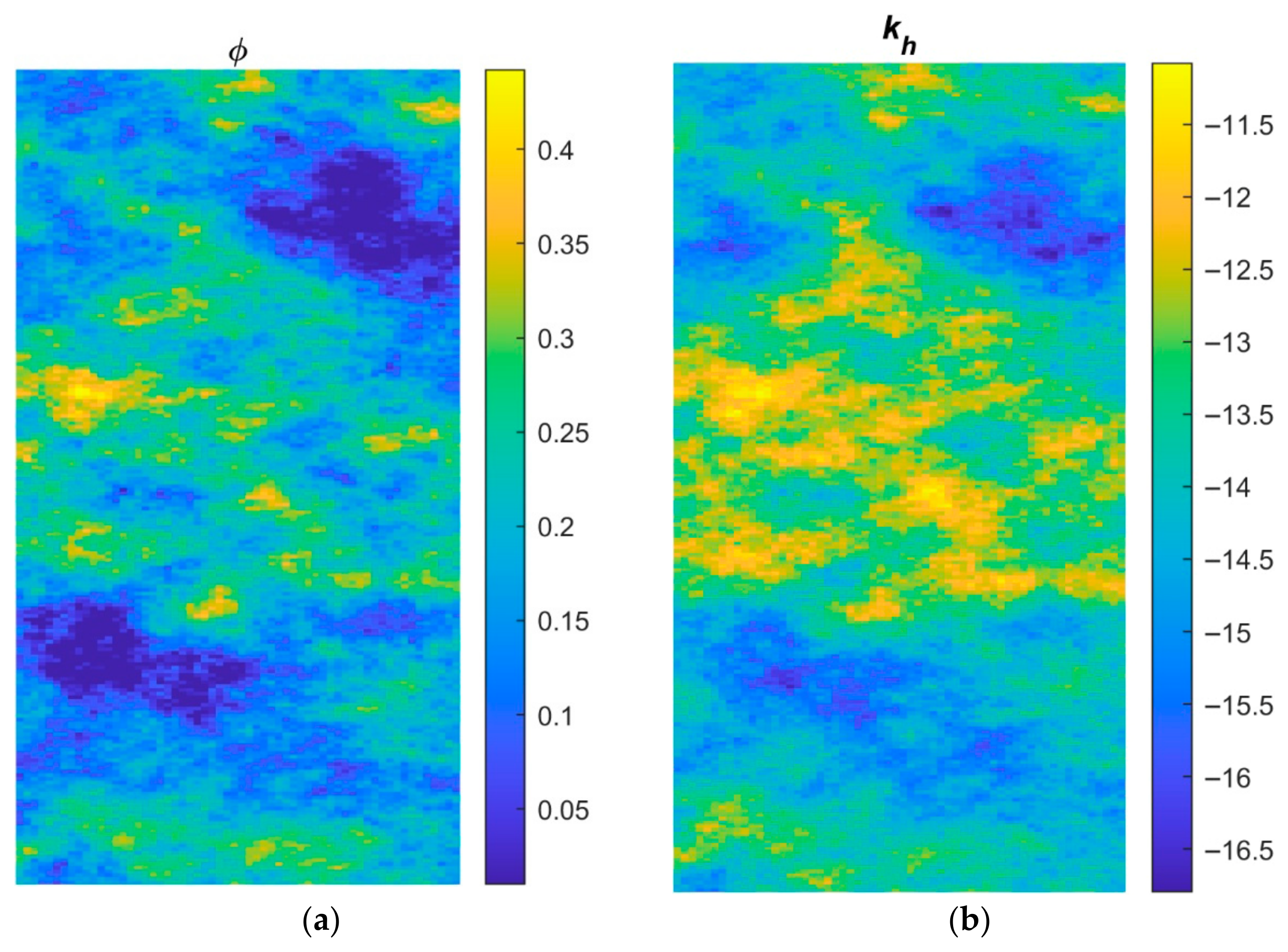
We consider one layer from the SPE10 dataset in the first case. Figure 1 shows the porosity and the logarithm of the absolute horizontal permeability field of the layer. The fine grid is discretized by a $60\times 220$ Cartesian grid. The physical model is an oil-water two-phase flow model, and the initial water and oil saturations are 0.2 and 0.8, respectively. The initial reservoir pressure is 41.369 MPa. There is one injection well located in the center of the domain and four producers in the four corners. The injection well injects water at a constant rate of 7.4428 m³/day, and the production wells are produced at constant bottom-hole pressure of 27.579 MPa. These well-control settings serve as the testing schedule. The simulation time horizon was 2000 days that was divided into 75 time steps. To initialize the flow, a small time step size of 0.1172 day was used for the first two steps, and the time step size was then increased gradually to 30 days. The training data was generated by running a fine-scale simulation with oscillatory well controls that are created by adding 5% random variation around the prescribed bottom-hole pressure and 25% variation around the prescribed water injection rate.

Figure 1. Porosity (a) and logarithmic absolute horizontal permeability (b) of one layer of the SPE10 dataset.

Figure 2 shows the four coarse-grid partitions generated from the fine grid. The cookie-cutter partition was created by imposing a 6 × 22 Cartesian grid on the fine grid, corresponding to a 10-fold coarsening ratio in each direction. The other three partitions were constructed using cell-wise indicators—absolute permeability, velocity magnitude, and time-of-flight—as the basis for grouping cells. The generation procedures were identical for all three indicator-based cases, differing only in the choice of indicator. Specifically, fine cells were first divided into 10 bins according to the selected indicator, then small blocks were merged using the mergeBlocks2 algorithm in MRST. Next, blocks with indicator values exceeding a prescribed threshold were refined using refineGreedy2, followed by a second merging of small blocks. The lower bound on the volume of blocks is set as $N_L=50$ and the upper bound on the total amount of flow indicator through each grid block is set as $N_U=100$. This process produced 136, 138, and 124 coarse blocks for the permeability-, velocity-, and time-of-flight–based partitions, respectively. The number of tunable parameters of the four resulting CGNet models are 373, 490, 499 and 457. The resulting indicator-based partitions are generally irregular in shape, reflecting the strong heterogeneity of the petrophysical properties and the resulting complexity of the flow field. In the permeability-based case, partition boundaries tend to align with regions of contrasting permeability, grouping cells with similar permeability values. By contrast, the velocity-magnitude and time-of-flight–based partitions adapt more closely to the actual flow pattern, as they implicitly account for the influence of injection and production wells.

Figure 2. Coarse grid partition of the spe10 layer. From left to right: (a) cookie-cutter partition, (b) permeability-based partition, (c) velocity-magnitude partition and (d) time-of-flight based partition. The thick black lines are boundaries of coarse blocks. The colors in (b–d) indicate the respective cell-wise flow indicators.

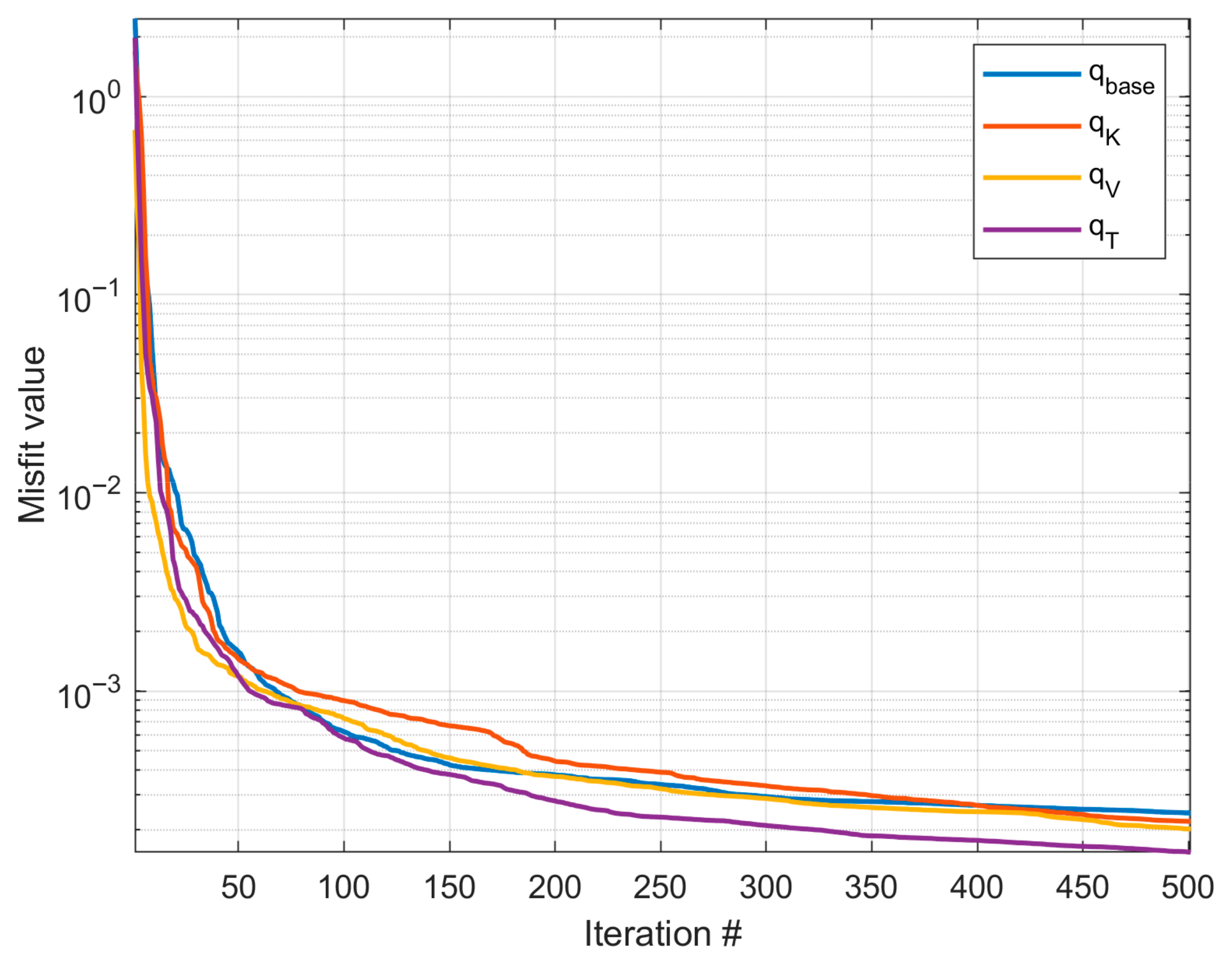
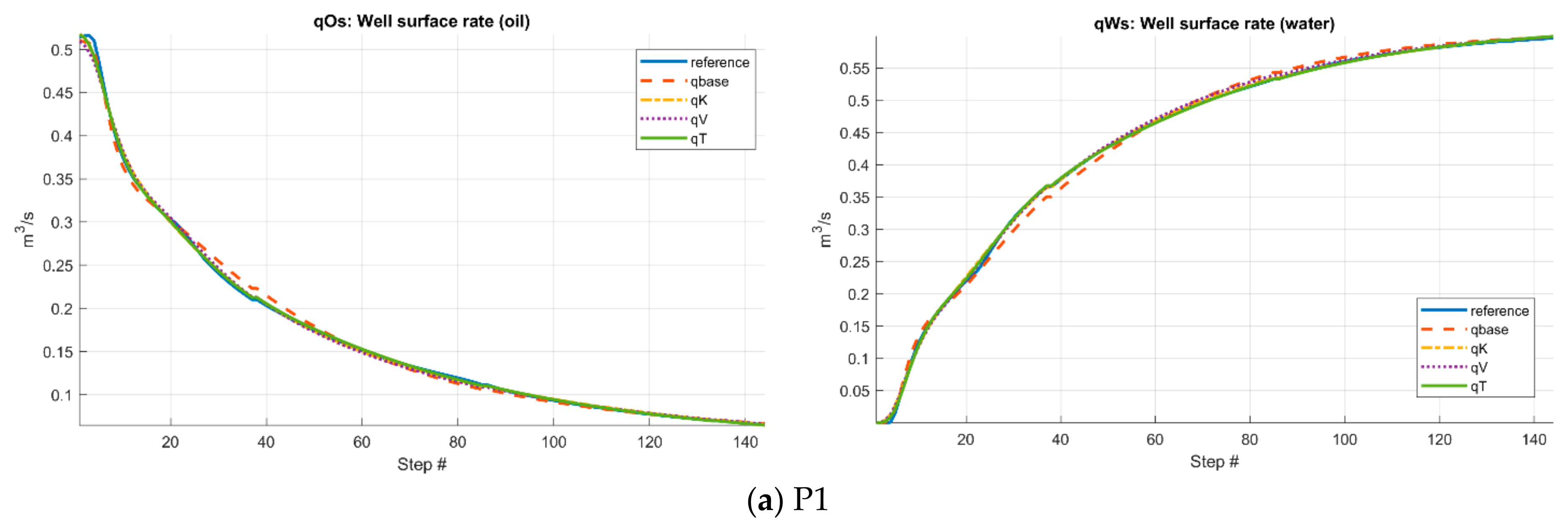
The weighting parameters in the misfit function are set as ${\omega }_p={10}^{-7}, {\omega }_w={10}^6, {\omega }_o={10}^6$ to scale the magnitudes of the different data points. The different CGNet models were trained for 500 iterations and Figure 3 shows the convergence plot of the misfit values during calibration. The base cookie-cutter partition, permeability-based partition, velocity-magnitude-based partition and the time-of-flight-based partition are denoted by $q_{\mathrm{base}}, q_K,q_V$ and $q_T$, respectively. Despite the huge differences in shape and graph topology of the four different CGNet models, their capabilities to match the calibration data are quite close to one another. All models display a steep reduction in misfit during the initial 50–100 iterations, followed by gradual convergence as the calibration progresses. This indicates that the optimization efficiently adjusts the tunable parameters during the early phase and then transitions to fine-tuning. The final misfit values of the four CGNet models are 0.0084, 0.0086, 0.0110 and 0.0096, respectively Figure 4 and Figure 5 display the predictions of bottom-hole pressure of the injection well and oil/water rates of the production wells using the four calibrated CGNet models for the testing well-control scenario. Compared to the fine-scale/reference solution, the quality of the four CGNet models are quite satisfactory. Except for the early period, the predictions of the CGNet models are very close to the reference solution. Particularly, the static cookie-cutter partition and the permeability-based partition are almost as good as the two flow-based partitions despite the fact that the two partitions do not account for the actual flow dynamics as do the velocity-magnitude and time-of-flight-based partition. Table 1 lists the accuracy metrics for the injection well and the four production wells computed using Equations (3) and (4). The results demonstrate the robustness of the CGNet models to the coarse partitions.

Figure 3. Misfit plot of different coarse-grid network models during calibration for the SPE10 layer.

Figure 4. Predictions of the bottom-hole pressure of the injection well using different CGNet models.

Figure 5. Predictions of oil and water rate of the production wells using different CGNet models for the SPE10 layer.

Table 1. Accuracy metric for the SPE10 layer.

	${\mathit{e}}_{\mathit{b}\mathit{h}\mathit{p}}$	${\mathit{e}}_{{\mathit{q}}_{\mathit{t}}}$				${\mathit{e}}_{{\mathit{f}}_{\mathit{w}}}$
	I1	P1	P2	P3	P4	P1	P2	P3	P4
$q_{base}$	5.88 × 10−3	1.03 × 10−2	7.60 × 10−3	2.47 × 10−3	1.05 × 10−2	2.72 × 10−3	2.09 × 10−3	7.74 × 10−4	1.04 × 10−3
$q_K$	4.20 × 10−3	1.02 × 10−2	7.77 × 10−3	4.08 × 10−3	1.31 × 10−2	2.91 × 10−3	2.00 × 10−3	5.36 × 10−4	1.18 × 10−3
$q_V$	3.76 × 10−3	1.05 × 10−2	1.05 × 10−2	3.05 × 10−3	1.07 × 10−2	3.03 × 10−3	1.84 × 10−3	6.57 × 10−4	1.68 × 10−3
$q_T$	7.26 × 10−3	1.27 × 10−2	1.18 × 10−2	5.28 × 10−3	1.02 × 10−2	3.33 × 10−3	1.99 × 10−3	8.63 × 10−4	1.48 × 10−3

3.2. Case 2: Norne Field

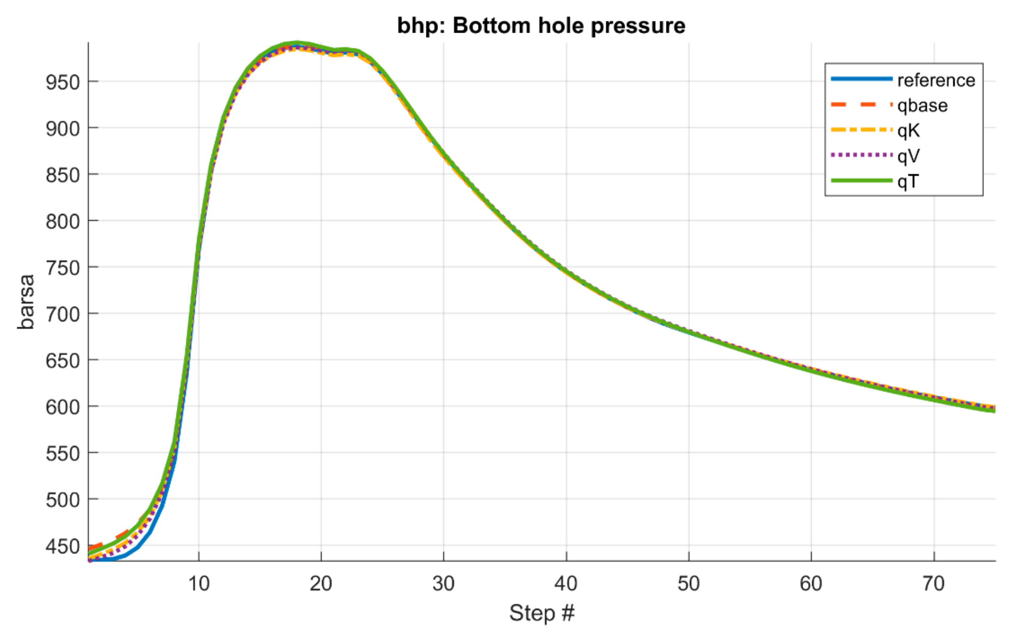
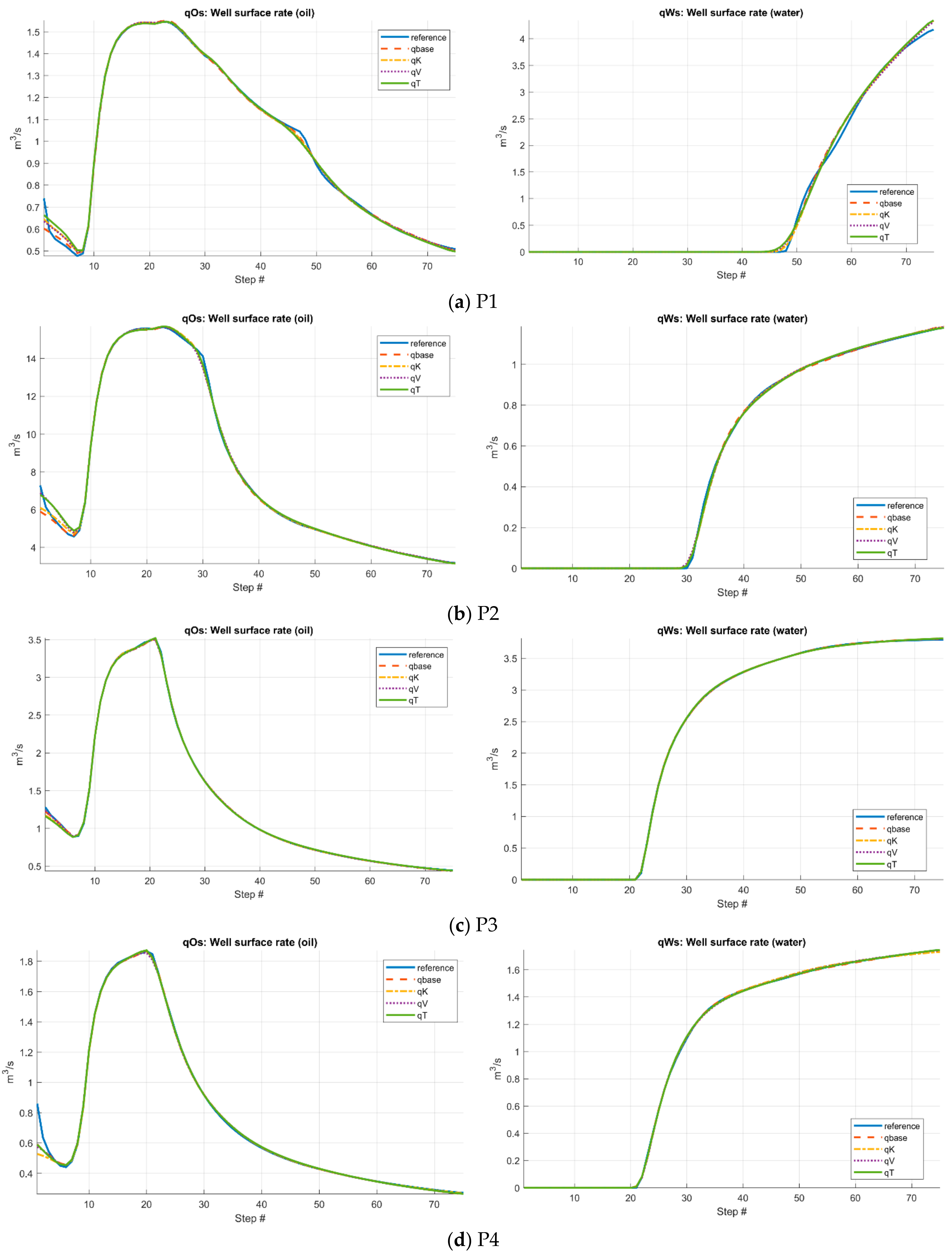
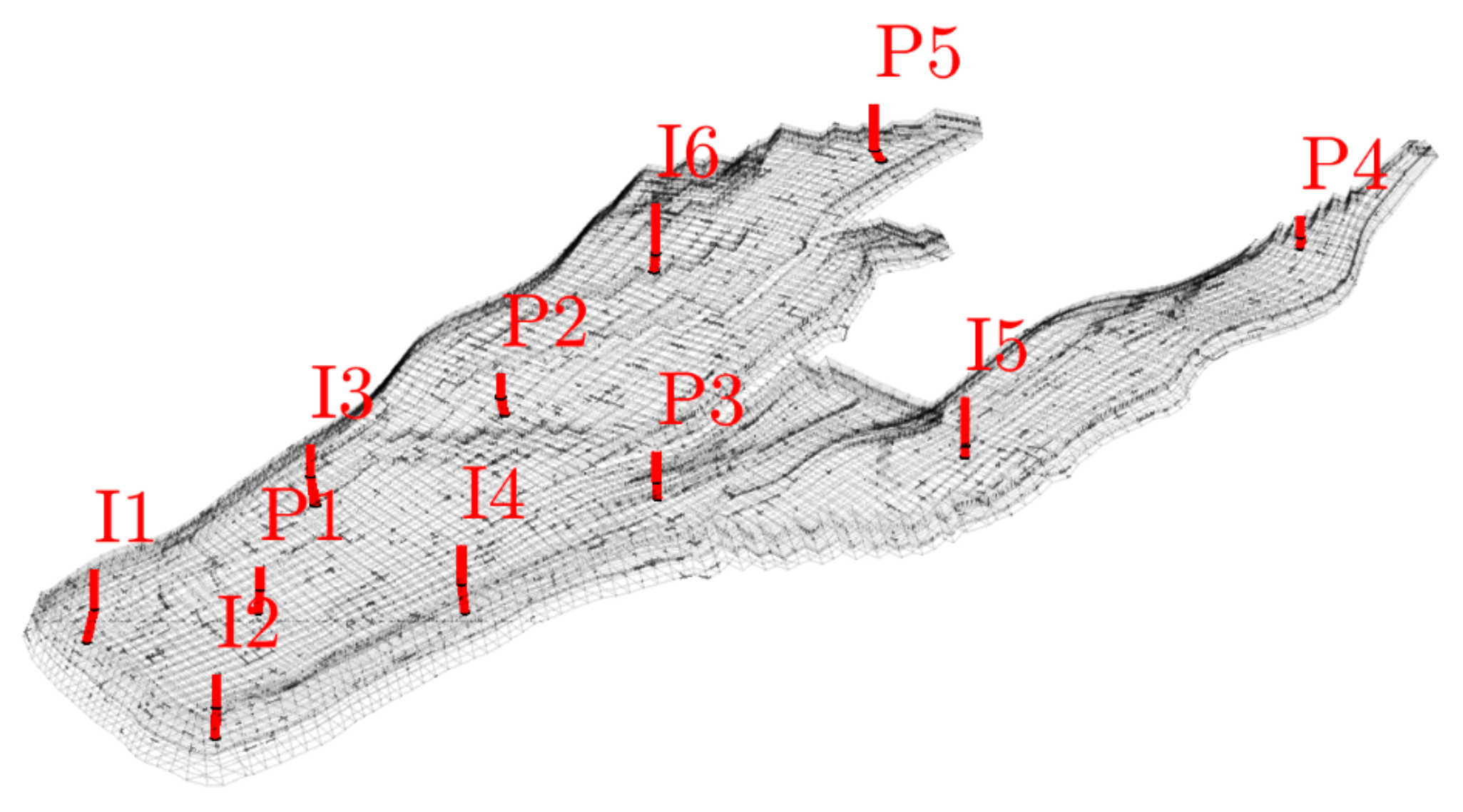
For the second test case, we consider the Norne field model from the Norwegian Sea, following the setup presented in [12]. The model represents a realistic field-scale reservoir and is publicly available. The reservoir geometry is defined on a 46 × 112 × 22 corner-point grid with 44,915 active cells and includes several structural complexities such as faults, displaced layers, and pinched-out cells. The petrophysical properties are highly heterogeneous, as illustrated in Figure 6, with horizontal permeability varying over nearly four orders of magnitude. The reservoir is initially oil-saturated, and water injection is applied to displace the dead oil under two-phase oil–water flow conditions. The dead-oil phase is modeled with a constant formation volume factor, and the oil and water viscosities are constant with a viscosity ratio of 5:1. Quadratic relative permeability curves with zero residual saturations are used for both phases. Production is achieved through five vertical producers operating at constant bottom-hole pressure, supported by six vertical injectors operating at constant rate (Figure 7). Similar to Case 1, the training data are generated from a fine-scale simulation using oscillatory well controls, obtained by superimposing ±5% random variations on the target bottom-hole pressures and ±25% variations on the injection rates. The resulting well schedules are shown in Figure 8.

Figure 6. Porosity distribution (a) and logarithmic horizontal permeability distribution (b).

Figure 7. Production and injection wells of the model denoted by the red thick lines. Well names are displayed next to the wells.

Figure 8. Well schedules used for generating calibration data (taken from Lie and Krogstad, 2023 [12]).

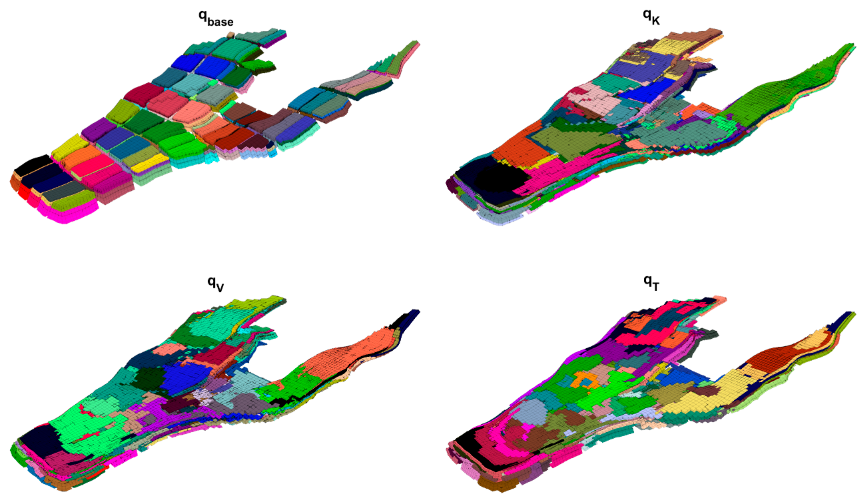
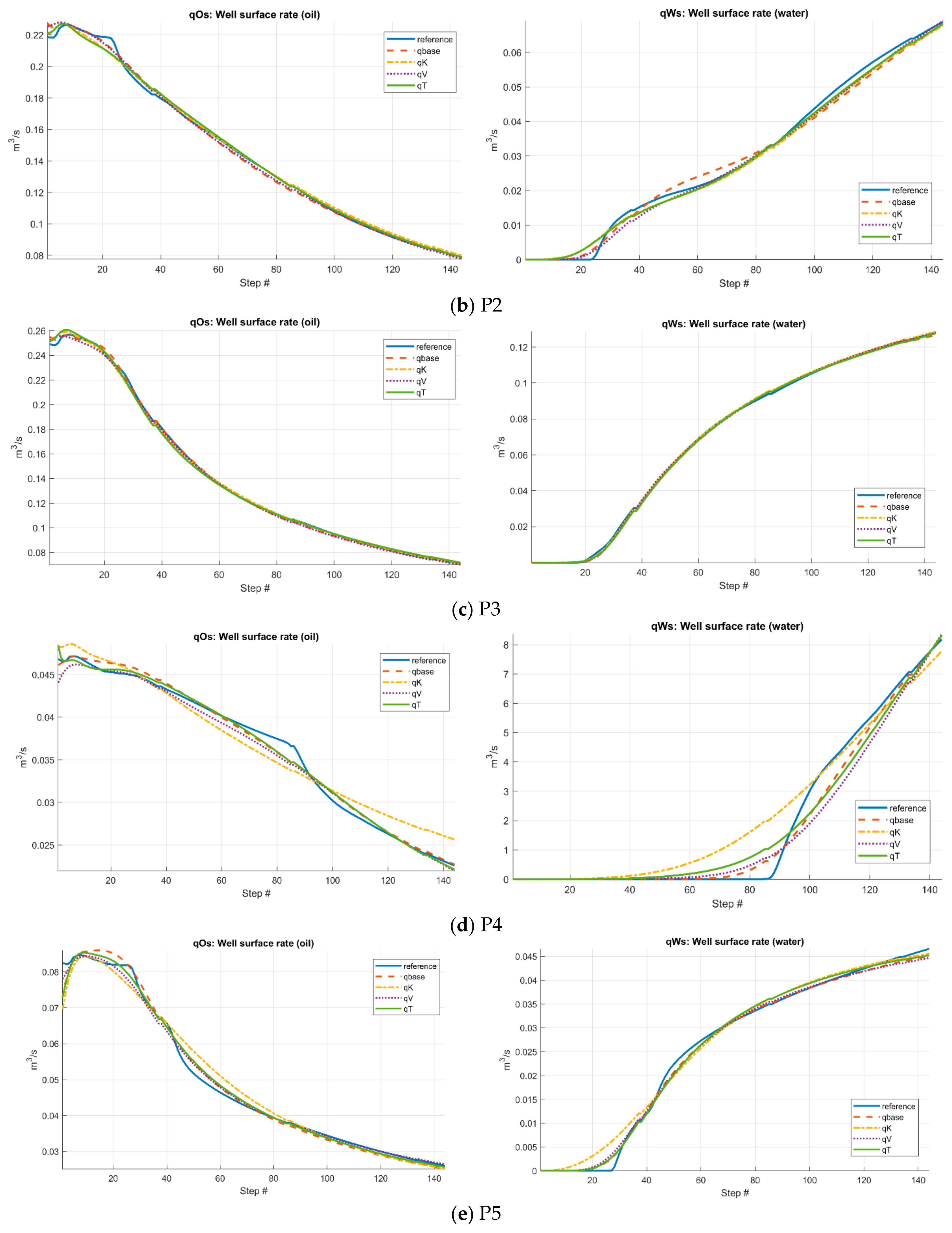
Figure 9 shows the four different coarse partitions of the underlying fine grid. The cookie-cutter partition is the simplest partition and serves as the baseline. It is generated in two steps: first a regular $8\times 9\times 2$ partition in index space, then followed by a split of disconnected blocks, leading to a total of 148 coarse grid blocks. The three cell-wise indicator-based coarse partitions are generated in a similar way as in case 1. The lower bound on the volume of blocks is set as $N_L=200$ and the upper bound on the total amount of flow indicator through each grid block is set as $N_U=300$, leading to a total number of coarse grid blocks of 145, 143, 144, respectively. The total number of tunable parameters for the four resulting CGNet models are 517, 1447, 1347 and 1107. Note that although the number of coarse blocks is similar, the number of tunable parameters for the three flow-indicator-based CGNet models is much higher than the simple cookie-cutter based CGNet model. The reason is that the irregularity of the flow-indicator-based CGNet models increases the number of connections among the coarse blocks. The weighting parameters in the misfit function are set as ${\omega }_p=2^{-8}, {\omega }_w=8.64, {\omega }_o=4.32$ to scale the magnitudes of the different data points. The resulting four coarse-grid network models are then trained for 500 iterations, and the misfit curves are displayed in Figure 10. The convergence behavior of the four CGNet models are quite similar, mirroring what was observed in the previous test case. However, for this test case, the CGNet model generated from the time-of-flight-based partition clearly matches the calibration data the best, although the magnitudes of the differences are not significant. The final misfit values of the four CGNet models are 7.50 × 10⁻⁴, 2.31 × 10⁻⁴, 2.84 × 10⁻⁴ and 1.73 × 10⁻⁴, respectively. Note that the magnitude of the misfit values in this case should not be compared to the previous case since the weighting parameters in the misfit function are different. Likewise, Figure 11 and Figure 12 show the predictions of bottom-hole pressure of injection wells and oil/water rate of production wells using the four CGNet models, respectively. The quality of bottom-hole pressure predictions is quite good, in general, for all CGNet models, with the prediction of the CGNet model generated from the simple cookie-cutter partition slightly off against the reference solution compared to the other three models. When it comes to the predictions of the oil/water rate of the production wells, the results are mixed: oil/water rates predictions are quite good for some production wells, but not so satisfactory for others. The predictions of water rate for well P4 are quite far off, with all four CGNet models failing to predict the water breakthrough time within acceptable accuracy. Refining the coarse partitions around the wells may improve the overall performance of the CGNet models. On the other hand, a close inspection of the results shows that the two CGNet models generated from the velocity-magnitude and time-of-flight-based partitions seem to be slightly better than the two CGNet models generated from the cookie-cutter partition and the permeability-based partition. In particular, the time-of-flight-based partition has the best overall performance, as can be seen in Table 2 and Table 3 where the accuracy metrics for the injection wells and production wells are listed, respectively. Therefore, taking into account the flow dynamics when generating the coarse grid partitions may be useful for complex reservoir models. This may be because the time-of-flight-based partition better captures the injector-producer connectivity as the flow field becomes more complex.

Figure 9. The four different coarse partitions. From top left to bottom right: Cookie-Cutter base partition (q_base), permeability-based partition (q_K), velocity-based partition (q_V) and time-of-flight-based partition (q_T). Different colors represent different coarse grid blocks.

Figure 10. Misfit plot of different coarse-grid network models during calibration for the Norne field.

Figure 11. Prediction of bottom-hole pressure of injection wells for the Norne field.

Figure 12. Prediction of oil and water rate of production wells for the Norne field.

Table 2. Accuracy metric for the bottom-hole pressures of the injection wells in Norne field model.

	I1	I2	I3	I4	I5	I6
$q_{base}$	7.24 × 10−3	8.03 × 10−3	8.90 × 10−3	1.13 × 10−2	4.07 × 10−3	6.07 × 10−3
$q_K$	4.14 × 10−3	3.44 × 10−3	3.53 × 10−3	2.38 × 10−3	1.84 × 10−3	2.21 × 10−3
$q_V$	6.25 × 10−3	3.96 × 10−3	6.65 × 10−3	5.35 × 10−3	3.21 × 10−3	4.12 × 10−3
$q_T$	5.57 × 10−3	2.26 × 10−3	5.27 × 10−3	1.95 × 10−3	1.46 × 10−3	2.34 × 10−3

Table 3. Accuracy metric for the total flow rate and water cut of the production wells in Norne field model.

	${\mathit{e}}_{{\mathit{q}}_{\mathit{t}}}$					${\mathit{e}}_{{\mathit{f}}_{\mathit{w}}}$
	P1	P2	P3	P4	P5	P1	P2	P3	P4	P5
$q_{base}$	5.98 × 10−3	1.22 × 10−2	3.12 × 10−3	1.07 × 10−2	1.86 × 10−2	8.06 × 10−3	8.24 × 10−3	3.64 × 10−3	5.60 × 10−3	7.58 × 10−3
$q_K$	2.51 × 10−3	4.09 × 10−3	7.30 × 10−3	3.62 × 10−2	2.35 × 10−2	3.31 × 10−3	8.26 × 10−3	1.84 × 10−3	1.58 × 10−2	1.80 × 10−2
$q_V$	4.83 × 10−3	1.12 × 10−2	5.88 × 10−3	1.64 × 10−2	8.60 × 10−3	3.76 × 10−3	5.64 × 10−3	3.62 × 10−3	9.60 × 10−3	8.46 × 10−3
$q_T$	2.92 × 10−3	6.23 × 10−3	8.03 × 10−3	9.63 × 10−3	1.28 × 10−2	2.19 × 10−3	5.98 × 10−3	3.04 × 10−3	8.89 × 10−3	9.09 × 10−3

4. Discussion

This work investigated how different coarse-grid partitioning strategies influence the accuracy and convergence behavior of CGNet proxy models. The results show that CGNet maintains a high level of predictive accuracy even when the coarse partitions differ significantly in shape, topology, and flow-structure representation. In the SPE10 case with strong permeability contrasts and channelized flow, the simple cookie-cutter and permeability-based partitions performed on par with the velocity- and TOF-based partitions, indicating that the calibration of transmissibilities and pore volumes can effectively compensate for geometric simplifications in many scenarios. This suggests that, for certain heterogeneous systems, preserving exact fine-scale flow paths in the coarse grid may be less critical than traditionally assumed in flow-based upscaling frameworks. In contrast, for the more operationally complex Norne case, the flow-guided partitions provided somewhat improved matches to production responses, implying that dynamic flow information becomes increasingly valuable when well interactions and multiphase displacement effects dominate system behavior. From a practical perspective, these findings highlight CGNet’s robustness and its potential as a surrogate modeling tool when time or computational constraints limit the ability to generate refined or flow-consistent partitions. Looking ahead, combining flow-aware indicators with topology-preserving strategies, and incorporating additional physical constraints during CGNet calibration, represent promising avenues for further enhancing the generality and interpretability of this proxy modeling approach.

5. Conclusions

This study investigated the impact of different coarse-grid partitioning strategies on the performance of coarse-grid network (CGNet) models developed within the MRST framework. Two numerical experiments were conducted using a single layer of the SPE10 benchmark model and a sector model of the Norne field. Four types of coarse partitions were tested: a simple cookie-cutter partition and three partitions generated based on cell-wise indicators—absolute permeability, velocity magnitude, and the product of forward and backward time-of-flight. Each resulting CGNet model was calibrated for 500 iterations to match reference well responses, and their convergence and predictive capabilities were analyzed in detail. The main conclusions are as follows:

• All CGNet models exhibited a rapid decline in the misfit function during the initial iterations, followed by gradual stabilization, indicating efficient parameter adjustment and numerical stability of the calibration process.
• In the SPE10 case, the final misfit values of the four CGNet models were very close (0.0084–0.0110) and the accuracy of well response predictions is also comparable among the four partitions, suggesting that the CGNet framework is robust to variations in partition geometry and topology. For the more geologically complex Norne field case, the model generated from the time-of-flight–based partition achieved the lowest misfit and slightly improved well-response predictions compared to the three partitions. This indicates that incorporating flow dynamics into partition generation may provide modest accuracy gains in heterogeneous reservoirs. However, the predictions of well responses for some production wells are still not satisfactory, especially in terms of water cut. Refining the coarse grid around the wells may improve the accuracy.

Overall, the study confirms that CGNet offers a computationally efficient, physically consistent, and flexible proxy modeling framework. It can achieve reliable accuracy with only limited coarse-grid resolution, making it suitable for large-scale optimization, history matching, and uncertainty quantification workflows.

References

1. Tang, M.; Liu, Y.; Durlofsky, L.J. Deep-learning-based surrogate flow modeling and geological parameterization for data assimilation in 3D subsurface flow. Comput. Methods Appl. Mech. Eng. 2021, 376, 113636. [Google Scholar] [CrossRef]
2. Kim, Y.D.; Durlofsky, L.J. Neural network surrogate for flow prediction and robust optimization in fractured reservoir systems. Fuel 2023, 351, 128756. [Google Scholar] [CrossRef]
3. Mo, S.; Zhu, Y.; Zabaras, N.; Shi, X.; Wu, J. Deep Convolutional Encoder-Decoder Networks for Uncertainty Quantification of Dynamic Multiphase Flow in Heterogeneous Media. Water Resour. Res. 2019, 55, 703–728. [Google Scholar] [CrossRef]
4. Kim, Y.D.; Durlofsky, L.J. A Recurrent Neural Network–Based Proxy Model for Well-Control Optimization with Nonlinear Output Constraints. SPE J. 2021, 26, 1837–1857. [Google Scholar] [CrossRef]
5. Wen, G.; Li, Z.; Azizzadenesheli, K.; Anandkumar, A.; Benson, S.M. U-FNO—An enhanced Fourier neural operator-based deep-learning model for multiphase flow. Adv. Water Resour. 2022, 163, 104180. [Google Scholar] [CrossRef]
6. Zhang, J.; Kang, J.; Zhang, K.; Zhang, L.; Liu, P.; Liu, X.; Sun, W.; Wang, G. An efficient transformer-based surrogate model with end-to-end training strategies for automatic history matching. Geoenergy Sci. Eng. 2024, 240, 212994. [Google Scholar] [CrossRef]
7. Raissi, M.; Perdikaris, P.; Karniadakis, G.E. Physics-informed neural networks: A deep learning framework for solving forward and inverse problems involving nonlinear partial differential equations. J. Comput. Phys. 2019, 378, 686–707. [Google Scholar] [CrossRef]
8. Yan, X.; Lin, J.; Wang, S.; Zhang, Z.; Liu, P.; Sun, S.; Yao, J.; Zhang, K. Physics-informed neural network simulation of two-phase flow in heterogeneous and fractured porous media. Adv. Water Resour. 2024, 189, 104731. [Google Scholar] [CrossRef]
9. Fuks, O.; Tchelepi, H.A. Limitations of physics informed machine learning for nonlinear two-phase transport in porous media. J. Mach. Learn. Model. Comput. 2020, 1, 19–37. [Google Scholar] [CrossRef]
10. Grossmann, T.G.; Komorowska, U.J.; Latz, J.; Schönlieb, C.-B. Can physics-informed neural networks beat the finite element method? IMA J. Appl. Math. 2024, 89, 143–174. [Google Scholar] [CrossRef] [PubMed]
11. Lie, K.-A.; Krogstad, S. Data-driven modelling with coarse-grid network models. Comput. Geosci. 2024, 28, 273–287. [Google Scholar] [CrossRef]
12. Lie, K.-A.; Krogstad, S. Comparison of two different types of reduced graph-based reservoir models: Interwell networks (GPSNet) versus aggregated coarse-grid networks (CGNet). Geoenergy Sci. Eng. 2023, 221, 111266. [Google Scholar] [CrossRef]
13. Lie, K.-A. An Introduction to Reservoir Simulation Using MATLAB/GNU Octave: User Guide for the MATLAB Reservoir Simulation Toolbox (MRST); Cambridge University Press: Cambridge, UK, 2019. [Google Scholar]
14. Zhao, H.; Kang, Z.; Zhang, X.; Sun, H.; Cao, L.; Reynolds, A.C. INSIM: A Data-Driven Model for History Matching and Prediction for Waterflooding Monitoring and Management with a Field Application. In Proceedings of the SPE Reservoir Simulation Symposium, Houston, TX, USA, 23–25 February 2015. [Google Scholar]
15. Ren, G.; He, J.; Wang, Z.; Younis, R.M.; Wen, X.-H. Implementation of Physics-Based Data-Driven Models with a Commercial Simulator. In Proceedings of the SPE Reservoir Simulation Conference, Galveston, TX, USA, 10–11 April 2019. [Google Scholar]
16. Aslam, B.; Yan, B.; Lie, K.-A.; Krogstad, S.; Møyner, O.; He, X. A Novel Hybrid Physics/Data-Driven Model for Fractured Reservoir Simulation. SPE J. 2024, 29, 7029–7045. [Google Scholar] [CrossRef]
Disclaimer/Publisher’s Note: The statements, opinions and data contained in all publications are solely those of the individual author(s) and contributor(s) and not of MDPI and/or the editor(s). MDPI and/or the editor(s) disclaim responsibility for any injury to people or property resulting from any ideas, methods, instructions or products referred to in the content.
Article Metrics
Citations
Article Access Statistics
Multiple requests from the same IP address are counted as one view.