Exploring Kolmogorov–Arnold Networks for Unsupervised Anomaly Detection in Industrial Processes

Abstract

Designing reliable fault detection and diagnosis (FDD) systems remains difficult when only limited fault-free data are available. Kolmogorov–Arnold Networks (KANs) have recently been proposed as parameter-efficient alternatives to multilayer perceptrons, yet their effectiveness for unsupervised FDD has not been systematically established. This study presents a statistically grounded comparison of Kolmogorov–Arnold Autoencoders (KAN-AEs) against an orthogonal autoencoder and a PCA baseline using the Tennessee Eastman Process benchmark. Four KAN-AE variants (EfficientKAN-AE, FastKAN-AE, FourierKAN-AE, and WavKAN-AE) were trained on fault-free data subsets ranging from 625 to 250,000 samples and evaluated over 30 independent runs. Detection performance was assessed using Bayesian signed-rank tests to estimate posterior probabilities of model superiority across fault scenarios. The results show that WavKAN-AE and EfficientKAN-AE achieve approximately 90–92% fault detection rate with only 2500 samples. In contrast, the orthogonal autoencoder requires over 30,000 samples to reach comparable performance, while PCA remains markedly below this level regardless of data size. Under data-rich conditions, Bayesian tests show that the orthogonal autoencoder matches or slightly outperforms the KAN-AEs on the more challenging fault scenarios, while remaining computationally more efficient. These findings position KAN-AEs as compact, data-efficient tools for industrial fault detection when historical fault-free data are scarce.

1. Introduction

Fault detection and diagnosis (FDD) is essential for maintaining safe, efficient, and sustainable industrial operations. Equipment malfunctions, sensor degradation, and control system anomalies can jeopardize safety, reduce productivity, and cause environmental harm. Although faults cannot always be prevented, process monitoring systems can detect deviations from normal operation and enable timely intervention [1,2]. A central challenge in industrial process monitoring lies in designing FDD methods that remain reliable under multivariate, dynamic, and drifting conditions [3]. The advent of Industry 4.0 has expanded sensor deployment across process units, producing large volumes of high-resolution multivariate data [4]. This abundance of data has shifted research toward data-driven frameworks that infer system behavior directly from measurements [5]. Data-driven frameworks encompass a wide range of approaches, from classical methods such as principal component analysis (PCA) [6,7] to machine learning models based on artificial neural networks (ANNs), including multilayer perceptrons (MLPs) [8,9], convolutional neural networks (CNNs) [10,11], and recurrent neural networks (RNNs) [5,12].

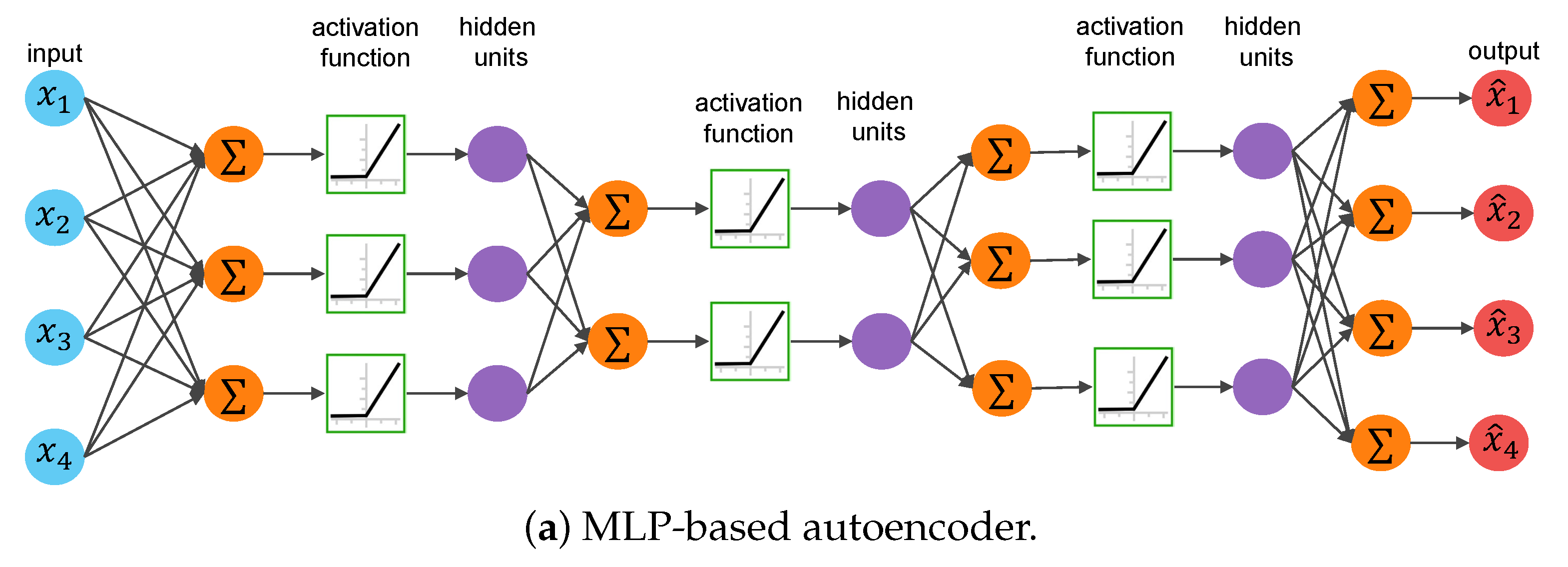
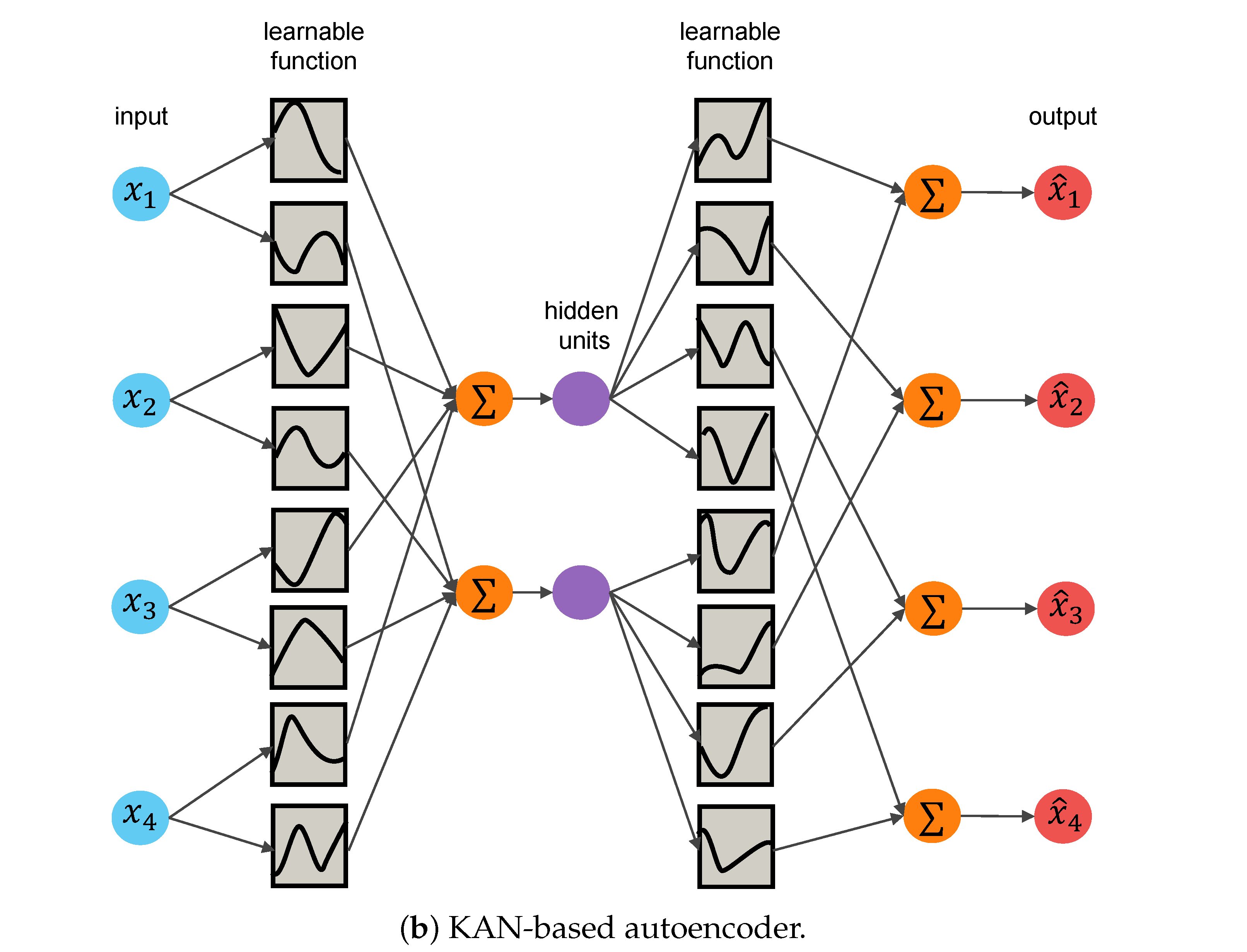
Despite their success, ANN-based FDD methods face persistent drawbacks. They typically require large datasets to achieve reliable performance, and their black-box nature hinders interpretability [13,14]. Motivated by these concerns, Liu et al. [15] introduced the Kolmogorov–Arnold Networks (KANs) as parameter-efficient and potentially more transparent alternatives to the traditional MLPs. In a KAN, each connection is parameterized by a learnable univariate function, and each node sums its transformed inputs [16]. This architecture appears interpretable because every transformation is explicit and can be examined individually. However, interpretability declines with depth: multilayer compositions of univariate functions generate complex, non-unique mappings that are difficult to analyze [15,17]. Although KANs only partially fulfill their interpretability promise, empirical evidence indicates that they remain effective as parameter-efficient models [18,19,20], motivating their application to supervised and unsupervised FDD tasks.

Recent research has applied KANs to unsupervised anomaly detection by integrating them with convolutional and recurrent architectures. Tang et al. [21] introduced a KAN-enhanced U-Net with mask-constrained reconstruction for surface defect localization, while Li et al. [22] proposed a temporal KAN autoencoder that incorporates domain knowledge into reconstruction error analysis for pipeline leak detection. For time-series anomaly detection, Wu et al. [23] combined CNN, LSTM, and KAN modules with residual filtering to monitor UAV sensors, achieving higher true positive and lower false positive rates than competing models. These efforts highlight the potential of KANs to enhance unsupervised anomaly detection through hybrid designs, though the capabilities and limitations of standalone KAN models in this setting remain largely underexplored.

KANs have also been applied to supervised FDD, often serving as lightweight classifiers. Rigas et al. [24] employed shallow KANs for rotating machinery fault diagnosis, achieving high F1-scores with far fewer parameters than deep network baselines. Cabral et al. [25] developed KANDiag, a KAN-based model for oil-immersed transformer fault diagnosis under imbalanced data conditions, achieving improved accuracy over standards methods. Hybrid architectures have further combined KANs with signal processing and deep feature extraction. For instance, He and Mo [26] paired wavelet time-frequency analysis with KAN classification, while Siddique et al. [27] fused wavelet coherent analysis and S-transform scalograms with a CNN-KAN model for centrifugal pump fault diagnosis, reporting near-perfect accuracy across multiple datasets. For structural and HVAC applications, Yan et al. [28] proposed KoCG-Net, a CNN–GRU–KAN model for impact-induced damage detection, outperforming baseline models in accuracy and noise robustness under data-limited conditions. Zhang et al. [29] introduced Conv-KAN for refrigerant fault diagnosis in variable refrigerant flow (VRF) systems. Collectively, these studies show that KANs act as parameter-efficient classifiers whose integration with domain-specific preprocessing or deep feature extraction yields competitive FDD performance.

Despite growing interest, current KAN-based FDD research still faces several open challenges: (1) most studies use the original B-spline formulation, while alternative basis families (e.g., wavelets, Fourier modes, Chebyshev polynomials) remain underexplored; (2) research has focused mainly on supervised tasks, with limited attention to unsupervised fault detection; (3) the impact of training set size on fault detection performance has not been systematically investigated; and (4) multi-seed statistical testing to distinguish genuine improvements from random fluctuations is rarely performed. To address these issues, we conduct a systematic evaluation of Kolmogorov–Arnold Autoencoders (KAN-AEs) for unsupervised fault detection in chemical process systems, using the Tennessee Eastman Process benchmark as a representative industrial case. We compare four KAN-AE variants, EfficientKAN-AE, FastKAN-AE, FourierKAN-AE, and WavKAN-AE, against an orthogonal autoencoder and PCA baseline, with each model trained and evaluated independently over 30 runs.

This study contributes to advancing KAN-based fault detection in three distinct ways: (1) the influence of functional parameterization in KAN edge functions on fault sensitivity is investigated by comparing the fault detection performance of different KAN-AE variants; (2) the data efficiency of KAN-AEs is evaluated by analyzing how fault detection performance scales with training set size, offering practical insight into the amount of data required for optimal detection; (3) model comparisons are statistically grounded through Bayesian signed-rank testing analysis to quantify probabilities of model superiority or practical equivalence.

The remainder of this paper is organized as follows: Section 2 introduces the theoretical background on PCA, autoencoders, and Kolmogorov–Arnold Networks. Section 3 details the experimental setup, including the Tennessee Eastman Process benchmark, model training procedures, fault detection strategy, and performance evaluation. Section 4 presents and analyzes the experimental results. Finally, Section 5 summarizes the key findings and outlines implications for industrial fault detection.

2. Preliminaries

This section outlines the modeling approaches used in this study: PCA, the conventional autoencoder, and its KAN extension.

2.1. Principal Component Analysis

Principal component analysis (PCA) is a linear dimensionality-reduction method introduced by Pearson [30] and later formalized by Hotelling [31]. This method remains widely used in process monitoring due to its simplicity, interpretability, and computational efficiency [32]. PCA is commonly performed on the standardized data matrix $X\in {\mathbb{R}}^{n\times m}$ via Singular Value Decomposition (SVD). The loading matrix $P\in {\mathbb{R}}^{m\times k}$ is obtained by retaining the k leading right singular vectors, which define the latent subspace. The score matrix $T\in {\mathbb{R}}^{n\times k}$ is then computed by projecting the original data onto this subspace, $T=XP$. Thus, the data matrix can be decomposed as:

$$X=T{P}^{\mathrm{T}}+E,$$

(1)

where $E\in {\mathbb{R}}^{n\times m}$ is the residual matrix capturing the variance unexplained by the model.

2.2. Autoencoders

Autoencoders (AEs) are neural networks that learn low-dimensional representations of high-dimensional data by reconstructing inputs from compressed latent variables. Compared with linear methods such as PCA or PLS, autoencoders capture the nonlinear dependencies common in chemical process data [33]. An AE consists of an encoder–decoder pair trained to minimize the mean squared reconstruction error:

$$\mathcal{L}(x,\widehat{x})={\displaystyle \frac{1}{N}}\sum _{i=1}^N{∥x_i-g\left(f\left(x_i\right)\right)∥}_2^2,$$

(2)

where $f(·)$ and $g(·)$ denote the encoder and decoder, respectively. The orthogonal autoencoder (OAE) [8] extends this formulation by adding a penalty that enforces decorrelation among latent dimensions:   

$${\mathcal{L}}_{\mathrm{OAE}}(x,\widehat{x})={\displaystyle \frac{1}{N}}\sum _{i=1}^N{∥x_i-g\left(f\left(x_i\right)\right)∥}_2^2+\lambda {∥Z^{\top }Z-I∥}_F^2,$$

(3)

where $Z\in {\mathbb{R}}^{N\times k}$ is the matrix of latent representations for a mini-batch of N samples and k latent features, $I\in {\mathbb{R}}^{k\times k}$ is the identity matrix, and $\lambda$ controls the regularization strength.

2.3. Kolmogorov–Arnold Networks

The Kolmogorov–Arnold Network (KAN) is a neural architecture inspired by the Kolmogorov–Arnold representation theorem [15]. Unlike conventional neural networks, which use fixed activation functions at nodes, KANs employ learnable activation functions on edges. A KAN layer transforms its input by applying learnable univariate functions to each feature and summing the results. Each connection from neuron j in layer $\ell -1$ to neuron i in layer ℓ is associated with a function ${\varphi }_{ij}^{(\ell )}:\mathbb{R}\to \mathbb{R}$. The output of neuron i is then given by:

$$x_i^{(\ell )}=\sum _{j=1}^{n_{\ell -1}}{\varphi }_{ij}^{(\ell )}\left(x_j^{(\ell -1)}\right),$$

(4)

where each ${\varphi }_{ij}^{(\ell )}$ is parameterized using a smooth basis expansion (e.g., B-splines, Gaussian RBFs). In this work, we focus on four representative KAN variants: Efficient-KAN, Fast-KAN, Fourier-KAN, and Wav-KAN, which are detailed in Appendix A.

2.4. Kolmogorov–Arnold Autoencoders

Kolmogorov–Arnold autoencoders (KAN-AEs) extend conventional autoencoders by replacing the dense layers in the encoder-decoder pair with KAN layers, as illustrated in Figure 1. Each connection in a KAN-AE learns its own transformation, allowing complex nonlinearities to be captured without deeper or wider architectures. KAN-AEs can be fully KAN-based [34] or hybrid, combining KAN and MLP layers [35]. In this study, all KAN-AEs employ only KAN layers, ensuring that performance differences can be attributed to the KAN architecture.

3. Methodology

This section presents the methodological framework used to configure, train, and evaluate the autoencoder models developed in this study. The analysis compares conventional and KAN-based autoencoders for unsupervised fault detection under matched conditions. All models were evaluated on the Tennessee Eastman Process (TEP), a widely adopted benchmark that provides a diverse and representative suite of industrial fault scenarios.

3.1. Case Study: The Tennessee Eastman Process

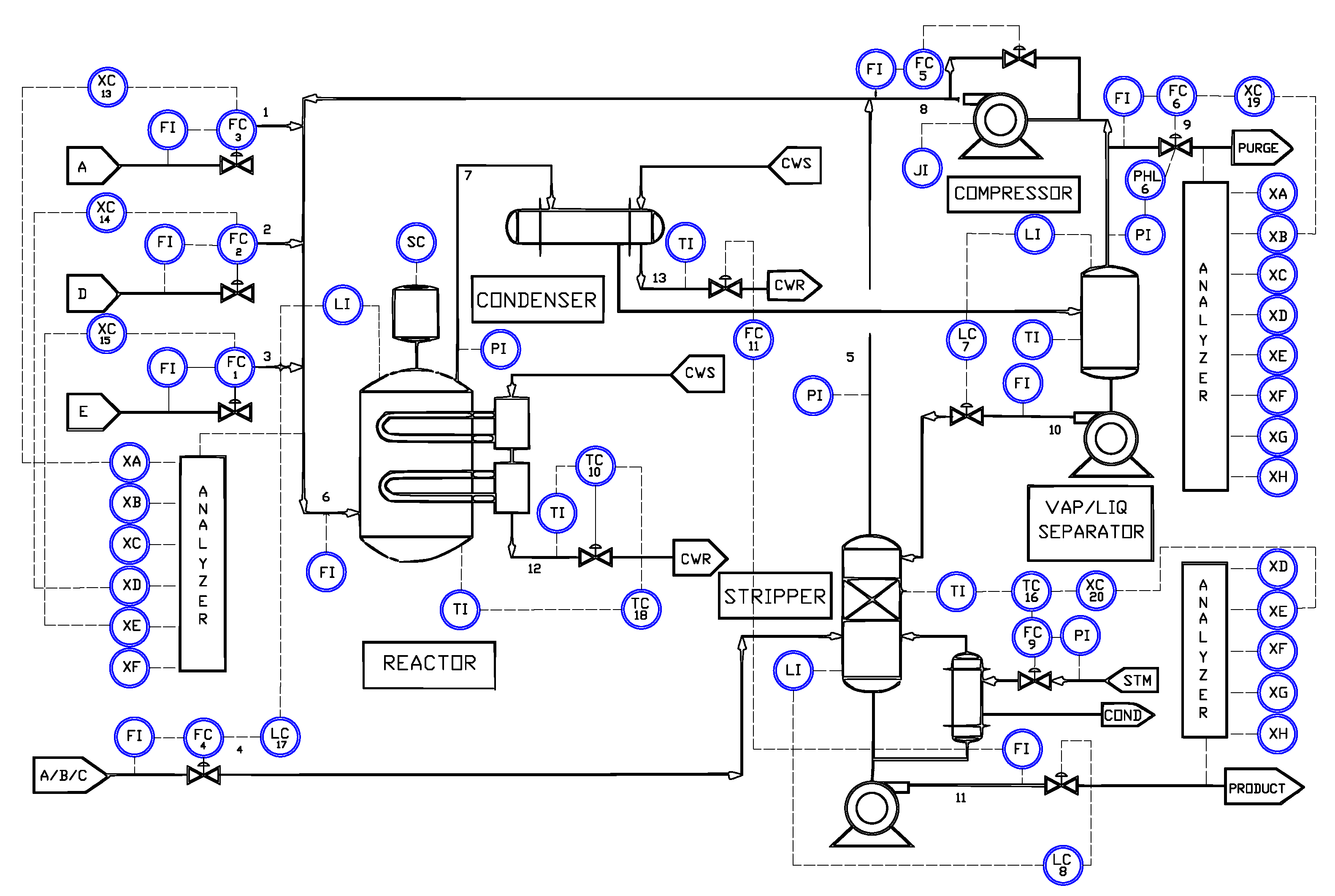
The Tennessee Eastman Process (TEP) serves as a widely used benchmark for process monitoring, providing a realistic yet controlled representation of a chemical plant. Originally introduced by Down and Vogel [36], it models a production system comprising eight chemical components and five interconnected process units (Figure 2). The process involves two primary exothermic reactions ($\mathrm{A}+\mathrm{C}+\mathrm{D}\to \mathrm{G}$ and $\mathrm{A}+\mathrm{C}+\mathrm{E}\to \mathrm{H}$) and two secondary byproduct reactions ($\mathrm{A}+\mathrm{E}\to \mathrm{F}$ and $3\mathrm{D}\to 2\mathrm{F}$), all occurring in the presence of an inert component ($\mathrm{B}$).

Researchers have developed multiple TEP implementations with different control strategies [37,38,39], leading to several publicly available datasets. In this study, we use the dataset of Rieth et al. [40] to train the models under varying data availability conditions, and the fault dataset of Russell et al. [41] to evaluate fault detection performance. The training set comprises 500 simulation runs under normal operating conditions, each containing 500 samples. The testing set includes one simulation run for each fault scenario, with measurements recorded every three minutes over a 48-h period (960 samples per run). In each fault simulation, the first 160 samples correspond to normal operation, and the remaining 800 samples represent the abnormal state. The dataset contains 11 manipulated variables, $\mathrm{XMV}\left(1\right)$–$\mathrm{XMV}\left(11\right)$, and 41 process measurements, $\mathrm{XMEAS}\left(1\right)$–$\mathrm{XMEAS}\left(41\right)$.

The benchmark includes 21 faults spanning diverse disturbance types.

Table 1. Summary of fault scenarios in the TEP benchmark, as reported in [36,41,42].

Fault	Type	Disturbed Value
1	Step	A/C ratio of stream 4, B composition constant
2	Step	B composition of stream 4, A/C ratio constant
3	Step	D feed (stream 2) temperature
4	Step	Cooling water inlet temperature of reactor
5	Step	Cooling water inlet temperature of separator
6	Step	A feed loss (stream 1)
7	Step	C header pressure loss (stream 4)
8	Random	A/B/C composition of stream 4
9	Random	D feed (stream 2) temperature
10	Random	C feed (stream 4) temperature
11	Random	Cooling water inlet temperature of reactor
12	Random	Cooling water inlet temperature of separator
13	Drift	Reaction kinetics
14	Stiction	Cooling water outlet valve of reactor
15	Stiction	Cooling water outlet valve of separator
16	Random	Deviations in heat transfer within stripper
17	Random	Deviations in heat transfer within reactor
18	Random	Deviations in heat transfer within condenser
19	Stiction	Recycle valve of compressor, underflow separator (stream 10), underflow stripper (stream 11), and steam valve stripper
20	Random	Deviations in flow rate (stream 7)
21	Constant position	Valve (stream 4)

summarizes each fault along with its identifier, disturbance type, and affected variable or mechanism. Faults 16–20 were originally labeled as unknown in the original benchmark; Bathelt et al. [42] later clarified the mechanisms for Faults 16–19, while Fault 20 was analyzed in our previous work [43], where its disturbance mechanism and process effects were described.

3.2. Data Preprocessing

We selected 33 process variables from the benchmark data. Variables $\mathrm{XMEAS}\left(23\right)$ to $\mathrm{XMEAS}\left(41\right)$, corresponding to analyzer measurements in the reactor feed, purge stream, and final product stream, were excluded because analyzer data are rarely available in real time [8]. Each observation corresponds to a single time step, and no temporal windowing was applied. In order to assess the data efficiency of the autoencoder models, we generated thirteen fault-free subsets ranging from 625 to 250,000 samples (see

Table 2. Subset sizes (prior to train/validation split) used for training autoencoder variants.

Description	Subset Sizes
Number of samples	625, 1250, 1875, 3125, 5000, 8125, 13 750,
	23 125, 38 125, 64 375, 107 500, 180 000, 250 000

). Each followed an 80/20 training-validation split. Furthermore, to preserve temporal structure, the data were split at the simulation level: entire simulation runs were randomly assigned to training and validation, truncating the last included run (in either partition) when necessary to match the target number of samples.

A z-score normalization scaler was fitted to the training set and applied consistently to both data partitions. The fitted scaler was saved and reused during inference to ensure consistent preprocessing. To support reproducibility, fixed random seeds were used for data partitioning and shared across model variants to ensure matched training conditions. Additional implementation details are provided in Section 3.4.

3.3. Process Monitoring Models

All models process input samples with 33 standardized features (see Section 3.1), following the benchmarking setup of Cacciarelli and Kulahci [8]. Consistent with that study, the PCA baseline retains 14 principal components, while the autoencoder models compress the inputs into a 25-dimensional latent space. Each autoencoder differs only in the parameterization of its encoder–decoder mappings and is trained to minimize the mean squared reconstruction error (Equation (2)), with additional regularization terms applied according to their architecture. Specifically, the OAE employs orthogonality regularization (Equation (3)), while EfficientKAN-AE introduces both L1 and entropy-based penalties (Equations (A3) and (A4)). Additionally, decoupled weight decay [44] is applied across all models as a shared regularization strategy.

Table 3. Summary of process monitoring model configurations.

Model	Attribute	Value
PCA	Layer sizes	[33, 14, 33]
	Function parameterization	Linear projection (SVD-based)
	No. of parameters	462
OAE	Layer sizes	[33, 85, 25, 85, 33]
	Function parameterization	Multilayer perceptron
	Activation function	ReLU
	Regularization	Orthogonality and weight decay
	No. of parameters	10,088
EfficientKAN-AE	Layer sizes	[33, 25, 33]
	Function parameterization	SiLU + B-spline expansion
	No. of basis functions	6
	Regularization	L1, entropy-based, and weight decay
	No. of parameters	11,550
FastKAN-AE	Layer sizes	[33, 25, 33]
	Function parameterization	SiLU + Gaussian RBF expansion
	No. of basis functions	5
	Regularization	Weight decay
	No. of parameters	10,074
FourierKAN-AE	Layer sizes	[33, 25, 33]
	Function parameterization	Fourier expansion
	No. of basis functions	7
	Regularization	Weight decay
	No. of parameters	9958
WavKAN-AE	Layer sizes	[33, 25, 33]
	Function parameterization	Single DoG wavelet
	Regularization	Weight decay
	No. of parameters	6716

summarizes the architectural and regularization settings.

3.4. Autoencoders Training Procedure

Each AE variant was trained independently on each subset of fault-free data (see Section 3.2), using 30 random seeds per configuration to capture stochastic effects from weight initialization and mini-batch sampling. This setup produced 390 independent training runs per model type.

Training employed the AdamW optimizer with a mini-batch size $B=256$ and a maximum of $E_{\max }=600$ epochs. Mixed-precision computation, enabled through PyTorch (v2.5.1+cu121) and its AMP module, accelerated training and reduced memory usage. A ReduceLROnPlateau scheduler decreased the learning rate after five validation epochs without improvement, and early stopping was triggered after 15 epochs without improvement. These settings were fixed across all AE variants. The initial learning rate ${\eta }_0$, weight decay, scheduler reduction factor, and regularization coefficients were tuned for each AE variant using the Tree-Structured Parzen Estimator (TPE) algorithm [45], implemented through the Optuna framework [46]. Hyperparameter optimization used a fixed subset of 625 fault-free samples with an 80/20 training-validation split. Because fault labels were not used during training, the validation reconstruction loss served as an unsupervised proxy for detection performance. The optimized hyperparameters for each model are summarized in

Table 4. Optimized training hyperparameters for each autoencoder variant (via TPE).

Model	Attribute	Value
OAE	Initial learning rate	$1.00\times {10}^{-3}$
	Weight decay	$1.00\times {10}^{-2}$
	Scheduler factor	0.20
	Orthogonality coefficient	1.00
EfficientKAN-AE	Initial learning rate	$4.38\times {10}^{-3}$
	Weight decay	$2.00\times {10}^{-2}$
	Scheduler factor	0.96
	L1 coefficient	$1.93\times {10}^{-4}$
	Entropy coefficient	$7.73\times {10}^{-4}$
FastKAN-AE	Initial learning rate	$1.92\times {10}^{-3}$
	Weight decay	$9.60\times {10}^{-3}$
	Scheduler factor	0.93
FourierKAN-AE	Initial learning rate	$3.63\times {10}^{-3}$
	Weight decay	$5.38\times {10}^{-3}$
	Scheduler factor	0.98
WavKAN-AE	Initial learning rate	$4.99\times {10}^{-3}$
	Weight decay	$7.60\times {10}^{-3}$
	Scheduler factor	0.95

.

Optimizing the hyperparameters for each architecture ensured that all models were evaluated under comparable and near-optimal conditions, enabling a fair and meaningful performance comparison.

3.5. Fault Detection

PCA-based models and autoencoders are widely used for fault detection in industrial systems, particularly when labeled fault data are scarce. Trained solely on normal process data, these models learn compact latent representations that enable accurate reconstruction of fault-free observations. Faults disrupt these learned patterns, leading to elevated reconstruction errors that signal abnormal behavior.

Two statistics are commonly employed in fault detection: the squared prediction error (SPE), or Q-statistic, and Hotelling’s $T^2$ statistic. The SPE measures the difference between an input and its reconstruction, whereas Hotelling’s $T^2$ quantifies deviations of latent features from the center of the fault-free distribution. Although both can be combined to improve sensitivity and robustness, this work focuses on the SPE.

For an input sample $x_i$, the SPE is defined as:

$$Q_i={\parallel x_i-{\widehat{x}}_i\parallel }_2^2,$$

(5)

where ${\widehat{x}}_i$ is the reconstruction of $x_i$. High $Q_i$ values indicate poor reconstruction, suggesting the presence of a fault.

A detection threshold $Q_{\lim }$ is obtained using kernel density estimation (KDE), a nonparametric approach that avoids assumptions about the distribution of SPE values and flexibly models nonlinear reconstruction behavior. The estimated probability density function $\widehat{P}\left(Q\right)$ is given by:

$$\widehat{P}\left(Q\right)={\displaystyle \frac{1}{nh}}\sum _{i=1}^{n}K\left({\displaystyle \frac{Q-Q_i}{h}}\right),$$

(6)

where $Q_i$ are the observed SPE values under normal conditions, $K(·)$ is a Gaussian kernel function, and h is the bandwidth determined via Scott’s Rule [47]:

$$h=\sigma n^{-1/5},$$

(7)

where $\sigma$ is the standard deviation of $Q_i$ values and n is the number of training samples.

The detection threshold $Q_{\lim }$ corresponds to the $(1-\alpha )$-quantile of the estimated density:

$$Q_{\lim }=inf\left\{x\mid {\int }_{-\infty }^x\widehat{P}\left(Q\right)dQ\ge 1-\alpha \right\},$$

(8)

where $\alpha$ is the significance level. In this study, we set $\alpha =0.05$, corresponding to an expected false alarm rate of approximately 5% under normal operating conditions.

3.6. Monitoring Performance Evaluation

Each trained model was evaluated on a fixed test set containing both fault-free and faulty samples. A sample was classified as normal or faulty according to the threshold $Q_{\lim }$; samples with $Q_i>Q_{\lim }$ are flagged as faulty.

Fault detection performance was quantified using two standard metrics: the fault detection rate (FDR) and the false alarm rate (FAR), defined as:

$$\mathrm{FDR}={\displaystyle \frac{\mathrm{TP}}{\mathrm{TP}+\mathrm{FN}}},$$

(9)

$$\mathrm{FAR}={\displaystyle \frac{\mathrm{FP}}{\mathrm{FP}+\mathrm{TN}}},$$

(10)

where TP, FP, FN, and TN denote the number of true positives, false positives, false negatives, and true negatives, respectively. FDR represents the proportion of actual faults correctly detected, while FAR measures the frequency of false alarms. Together, these metrics describe the trade-off between sensitivity and specificity. Robust detection requires models that maintain high FDR with consistently low FAR.

3.7. Computational Efficiency Benchmark

The computational efficiency of the monitoring nonlinear models in Table 3 was evaluated on the TEP dataset using the training configuration described in Section 3.4, including each model’s respective loss function and regularization terms. A dedicated PyTorch benchmarking routine was executed to measure the average forward and backward pass durations per batch on both CPU and GPU devices. Benchmarks were conducted on a workstation equipped with a 12th Gen Intel^® Core™ i9-12900H processor (20 cores, 2.5 GHz, 16 GB RAM) and an NVIDIA^® GeForce RTX 3070 Ti Laptop GPU (8 GB memory).

Each benchmark included 50 warm-up batches to stabilize hardware utilization, followed by 500 timed iterations. Forward and backward durations were recorded using CUDA events on the GPU and wall-clock timing on the CPU, and mean values with 95% confidence intervals were computed across timed batches to quantify runtime variability. Because KAN-based architectures are known to be computationally heavier than conventional neural networks [48,49,50] due to the evaluation of multiple basis functions along each network edge, performance is reported in terms of slowdown rather than speed-up. The OAE served as the baseline, and relative slowdown factors were computed by dividing each model’s mean forward or backward pass duration by that of the OAE on the same device. The resulting slowdown ratios and timing statistics are presented and discussed in Section 4.3.

3.8. Bayesian Signed-Rank Test for Model Comparison

While the FDR summarizes average performance, it does not reveal whether performance differences between models are statistically meaningful. To address this, we applied the Bayesian signed-rank test proposed by Benavoli et al. [51,52]. This method estimates the posterior probability that one model is practically superior to another across multiple fault scenarios, accounting for uncertainty in the results and defining a region of practical equivalence (ROPE) that treats small performance differences as negligible. In this study, the ROPE radius was set to $r=0.01$, corresponding to a $\pm 1\%$ absolute change in FDR.

For each model pair, the test yields three probabilities: $P_{\mathrm{left}}$ (model A better), $P_{\mathrm{rope}}$ (practically equivalent), and $P_{\mathrm{right}}$ (model B better). These probabilities provide a probabilistic assessment of relative model performance rather than a binary significance outcome.

4. Results and Discussion

4.1. Performance Scaling with Training Set Size

To understand how model performance varies across both fault type and data availability, we follow the classification proposed by Sun et al. [5], which distinguishes three fault categories: controllable, back-to-control, and uncontrollable. High FDR values are desirable for back-to-control and uncontrollable faults, as they indicate timely detection of abnormal behavior. In contrast, elevated FDRs for controllable faults may signal excessive sensitivity to normal fluctuations and result in unnecessary process interventions. An effective monitoring system should maintain the FDR near the nominal false alarm level for controllable faults while achieving high detection rates for the other two categories. Building on this distinction, training set sizes ($n_{\mathrm{train}}$) were grouped into three regimes: data-scarce ($n_{\mathrm{train}}<{10}^4$), data-sufficient (${10}^4\le n_{\mathrm{train}}\le {10}^5$), and data-rich ($n_{\mathrm{train}}>{10}^5$). For each model, FDRs were first averaged across faults within each category and then across training runs. 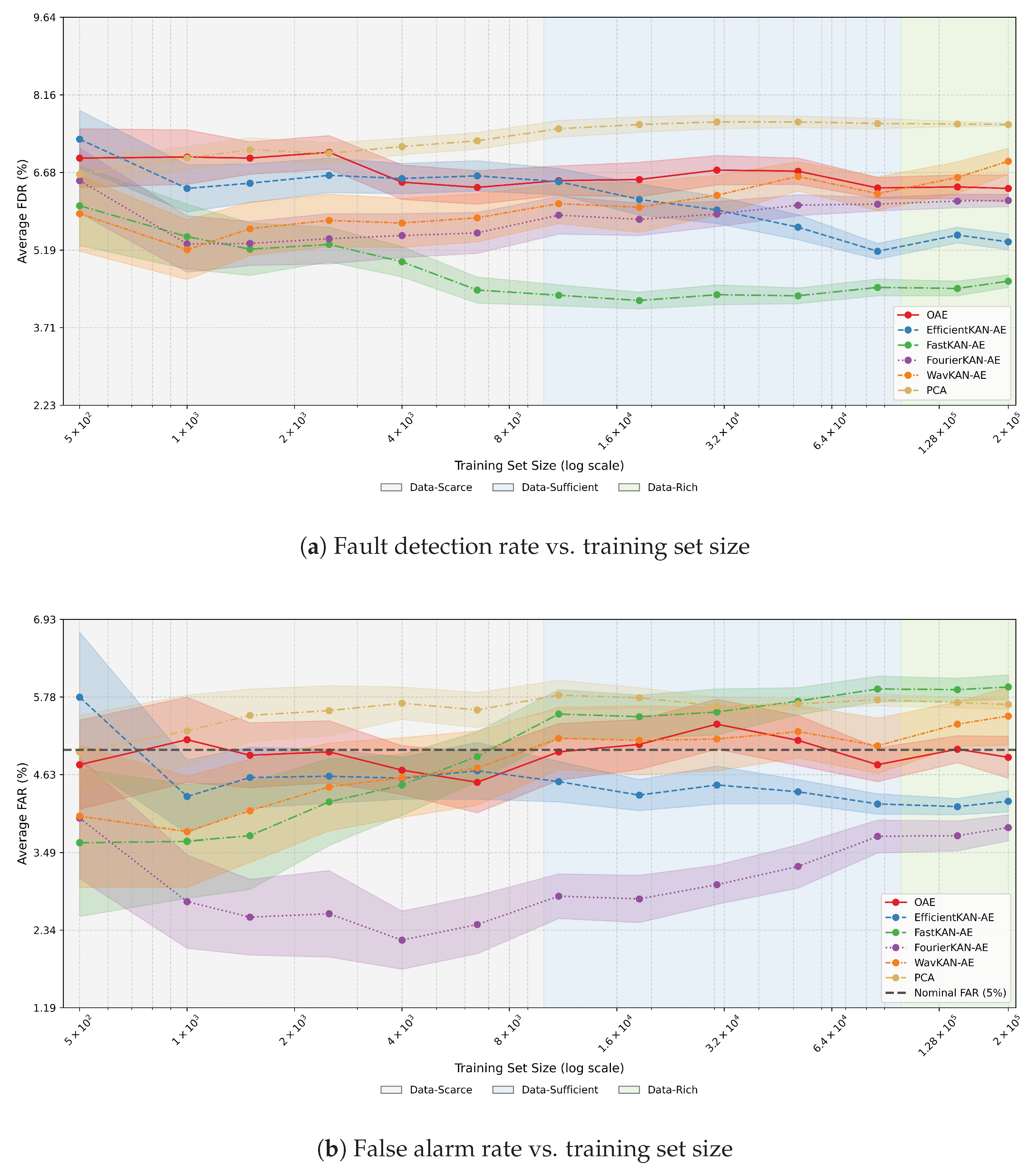Figure 3, Figure 4 and Figure 5 summarize these results, with shaded 95% confidence intervals representing variability across training runs.

4.1.1. Controllable Faults

For controllable faults, an ideal monitoring system should maintain a low and stable fault detection rate, as excessive alarms can lead to unnecessary interventions. Figure 3a summarizes FDR trends, indicating that the average rate for nonlinear models remained within a narrow 4–5.5% range across all training regimes. This consistency shows that increasing the amount of fault-free data had little influence on sensitivity to minor, self-correcting disturbances. Among nonlinear models, OAE displayed nearly constant performance, whereas EfficientKAN-AE showed a slight decline in FDR with larger datasets. FastKAN-AE achieved the strongest improvement, reaching an average FDR of 4.6% as $n_{\mathrm{train}}$ increased. In contrast, WavKAN-AE and FourierKAN-AE exhibited small FDR increases, implying mild over-sensitivity to nominal process variability.

The false alarm rates (see Figure 3b) complement these observations. EfficientKAN-AE and FourierKAN-AE consistently achieved the lowest FAR values (4–4.5%), while OAE and WavKAN-AE maintained slightly higher yet acceptable rates around 5%. Notably, FastKAN-AE exhibited a moderate rise in FAR at larger training sizes, suggesting a conservative detection bias. The PCA baseline performed worst on both metrics, yielding the highest FDR (≈7.6%) and FAR (≈5.7%) at higher data volumes. This underscores the advantage of nonlinear models in distinguishing normal fluctuations from genuine fault conditions.

4.1.2. Back-to-Control Faults

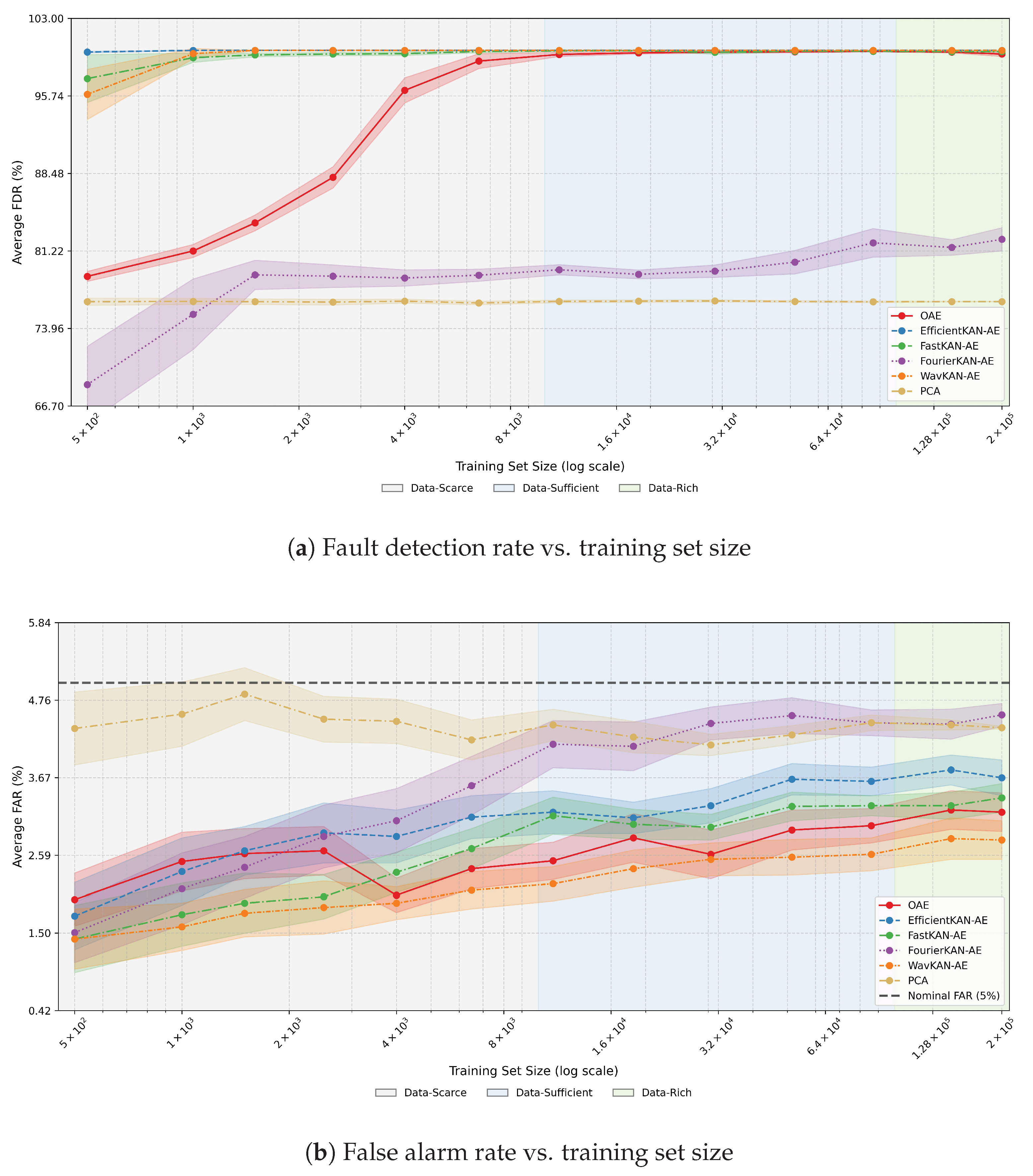
For back-to-control faults, high fault detection rates are desirable, as they reflect the model’s ability to detect persistent process deviations. Detection performance improved steadily with increasing $n_{\mathrm{train}}$ (Figure 4a). Among KAN-AE variants, EfficientKAN-AE and WavKAN-AE reached near-perfect FDRs with as few as 1000 samples and maintained this level thereafter, highlighting their strong data efficiency in capturing deviations in manipulated variables. FastKAN-AE followed a similar trajectory but required larger data volumes to reach peak performance, indicating reduced data efficiency in the data-scarce regime. The OAE model improved more gradually, attaining high FDRs only in the data-sufficient regime, suggesting that conventional orthogonal regularization benefits from larger sample diversity. In contrast, FourierKAN-AE consistently underperformed, with FDR values plateauing below those of the other models; this may result from the limited flexibility of its low-order global basis functions. Finally, the PCA baseline achieved a consistent, albeit limited, performance of approximately 76% regardless of data volume. Taken together, the results show that KAN-AEs achieve reliable detection of back-to-control faults with substantially fewer training samples than PCA and OAE, confirming their superior data efficiency for this fault category.

False alarm rates for all nonlinear models exhibited a modest upward trend with increasing $n_{\mathrm{train}}$ but remained substantially below the nominal FAR, holding between 2–4% (Figure 4b). This indicates that the FDR gains did not result in an undue increase in false positives. The PCA baseline maintained a FAR of approximately 4.5%, indicating satisfactory performance, though consistently below that of the nonlinear models.

4.1.3. Uncontrollable Faults

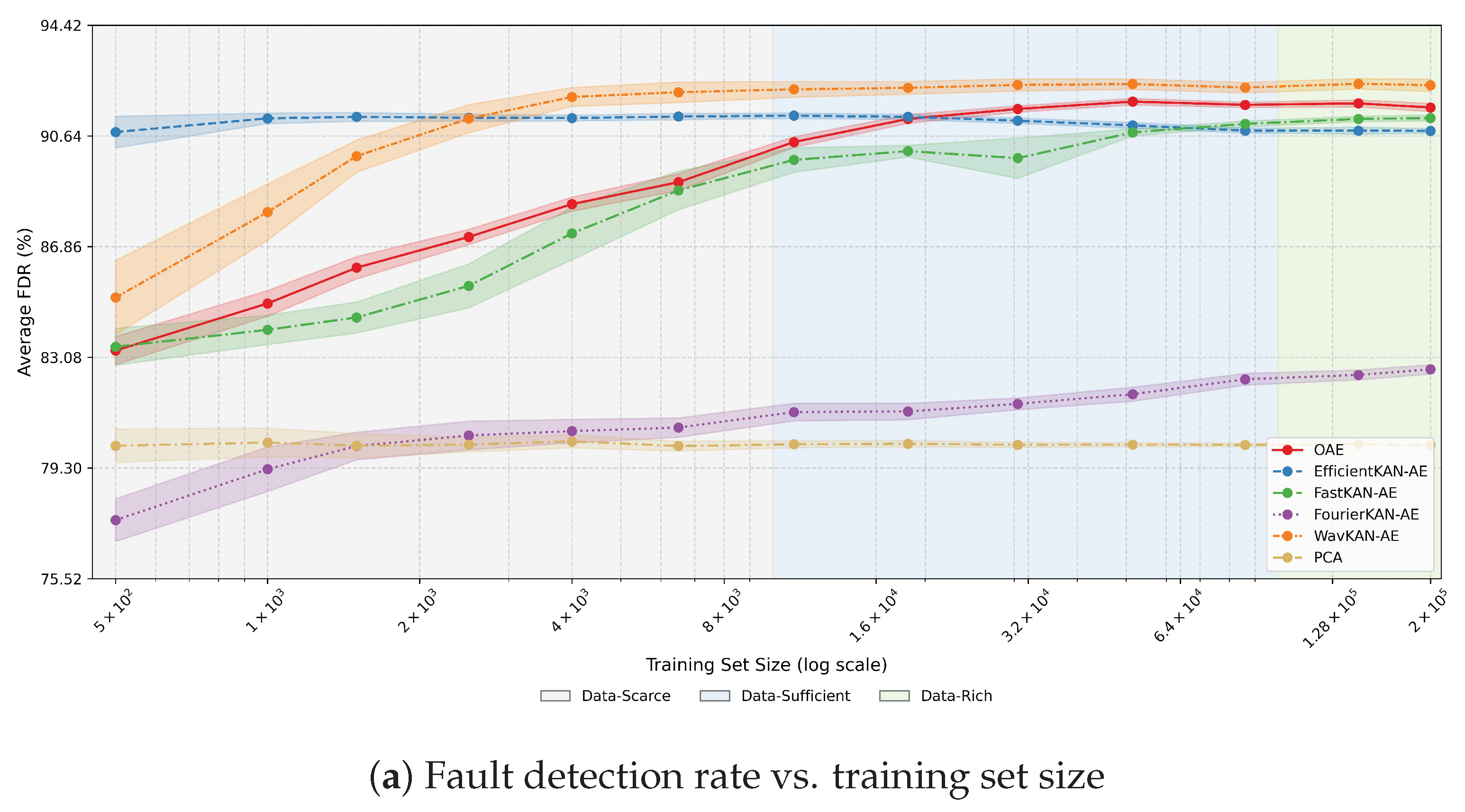
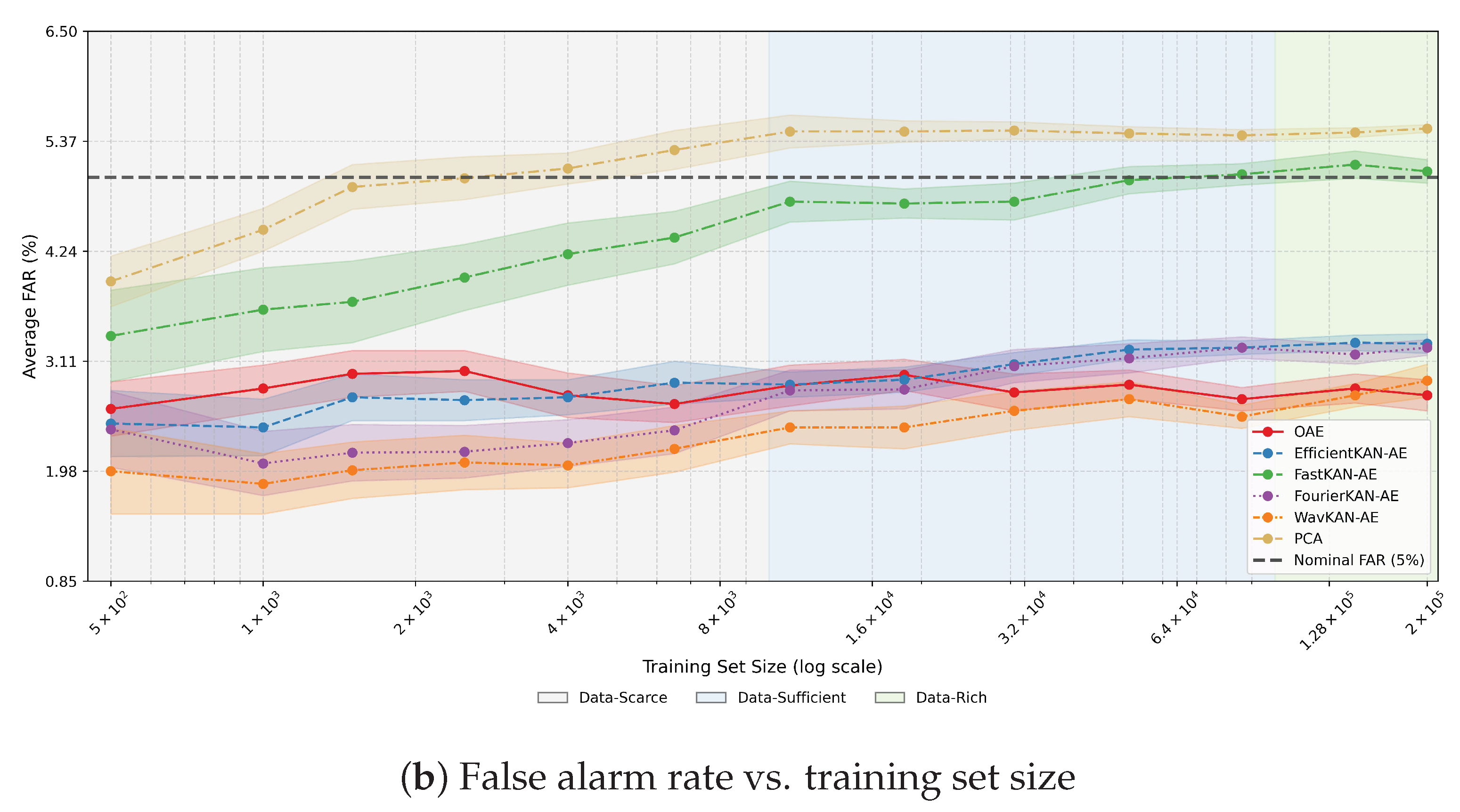
In the case of uncontrollable faults, high detection rates are essential, as these events represent severe process deviations that cannot self-correct. Detection performance improved consistently with increasing $n_{\mathrm{train}}$ across all nonlinear models, as illustrated in Figure 5a, although the rate and extent of improvement varied. EfficientKAN-AE achieved the highest initial FDR at $n_{\mathrm{train}}=500$ and maintained stable performance throughout, with only a minor dip in the data-sufficient regime, possibly due to over-regularization. WavKAN-AE started lower but improved rapidly, reaching over 92% FDR with just 2500 training samples, which demonstrates strong data efficiency and effective wavelet-based feature extraction. FastKAN-AE showed a slower response, with higher variability across runs and strong performance only in the data-rich regime. OAE improved gradually, achieving competitive FDRs in the data-sufficient regime but never surpassing WavKAN-AE even at larger data volumes. FourierKAN-AE consistently lagged behind, reflecting the limited expressivity of its global basis representation. The PCA baseline showed stable but much lower FDR (≈80%) across all training sizes. Overall, KAN-AEs demonstrated superior data efficiency in detecting uncontrollable faults. Note that these high FDR values did not lead to a substantial increase in false positives (see Figure 5b). All models maintained an acceptable FAR behavior, generally below the nominal 5% threshold. The nonlinear architectures showed stable performance within the 2–3% range, except for FastKAN-AE, which exhibited a mild increase approaching 5% in the largest data regime. PCA yielded slightly higher values around 4–5.5%. These results confirm that all models, particularly the KAN-AE variants, effectively distinguished severe faults from nominal operation.

4.2. Model Behavior Under Data-Scarcity (1000 Samples)

The previous analysis of monitoring performance trends averaged fault detection rate (FDR) values across the fault clusters defined by Sun et al. [5]. While this approach is useful for identifying overall model behavior as the amount of training data increases, it conceals model-specific differences among individual fault scenarios. In practice, assessing the robustness and generalization of monitoring models requires understanding which specific faults each model can detect reliably and which remain challenging. Accordingly, this subsection examines model behavior under a data-scarce regime using $n_{\mathrm{train}}=1000$ normal samples. The corresponding FDR results for each model and fault scenario are summarized in

Table 5. Fault Detection Rate (FDR) per fault for each model (1000 training samples). Values are reported as mean ± 95% confidence interval, expressed as percentages.

Fault	PCA	OAE	EfficientKAN-AE	FastKAN-AE	FourierKAN-AE	WavKAN-AE
3	6.17 ± 0.33	6.12 ± 0.62	5.35 ± 0.55	4.91 ± 0.70	4.28 ± 0.55	3.96 ± 0.60
9	6.57 ± 0.30	6.15 ± 0.57	5.37 ± 0.61	4.50 ± 0.62	3.43 ± 0.61	3.15 ± 0.65
15	8.12 ± 0.45	8.62 ± 0.72	8.40 ± 0.63	6.95 ± 0.66	8.21 ± 0.89	8.51 ± 0.90
4	100.00 ± 0.00	99.80 ± 0.25	99.99 ± 0.03	97.97 ± 1.33	91.75 ± 8.86	100.00 ± 0.00
5	29.51 ± 0.86	43.87 ± 1.78	100.00 ± 0.00	99.99 ± 0.01	34.14 ± 2.01	99.10 ± 1.48
7	100.00 ± 0.00	100.00 ± 0.01	100.00 ± 0.00	100.00 ± 0.00	100.00 ± 0.00	100.00 ± 0.00
1	99.93 ± 0.02	99.91 ± 0.03	99.66 ± 0.02	99.52 ± 0.03	99.61 ± 0.05	99.66 ± 0.04
2	97.88 ± 0.33	98.67 ± 0.07	98.54 ± 0.03	98.20 ± 0.06	98.52 ± 0.02	98.50 ± 0.00
6	100.00 ± 0.00	100.00 ± 0.00	100.00 ± 0.00	100.00 ± 0.00	100.00 ± 0.00	100.00 ± 0.00
8	92.42 ± 0.66	98.15 ± 0.12	98.12 ± 0.08	98.20 ± 0.08	97.92 ± 0.10	98.05 ± 0.13
10	43.36 ± 2.50	63.68 ± 2.11	86.28 ± 0.33	69.31 ± 0.98	49.71 ± 1.33	77.92 ± 1.37
11	82.10 ± 1.21	79.32 ± 1.13	70.02 ± 1.04	74.52 ± 1.04	76.89 ± 3.35	79.92 ± 1.36
12	93.81 ± 0.46	98.85 ± 0.08	99.50 ± 0.03	99.09 ± 0.03	98.77 ± 0.10	99.30 ± 0.11
13	95.42 ± 0.05	95.46 ± 0.09	94.87 ± 0.10	94.90 ± 0.08	94.44 ± 0.07	94.50 ± 0.07
14	100.00 ± 0.01	100.00 ± 0.01	100.00 ± 0.00	100.00 ± 0.01	100.00 ± 0.00	100.00 ± 0.00
16	41.97 ± 2.39	59.65 ± 1.95	89.26 ± 0.62	66.35 ± 1.16	38.32 ± 1.57	78.40 ± 1.68
17	96.30 ± 0.13	96.78 ± 0.20	93.95 ± 0.59	95.74 ± 0.19	93.03 ± 1.27	94.70 ± 0.51
18	90.85 ± 0.10	90.75 ± 0.15	90.00 ± 0.08	89.99 ± 0.09	90.10 ± 0.15	90.17 ± 0.14
19	29.39 ± 2.00	43.57 ± 2.84	84.44 ± 0.99	31.83 ± 4.91	20.55 ± 2.79	58.36 ± 7.14
20	58.93 ± 0.81	64.03 ± 0.90	72.67 ± 0.70	58.67 ± 1.26	51.78 ± 1.65	63.14 ± 2.10
21	51.74 ± 1.57	47.41 ± 1.94	47.42 ± 1.47	46.70 ± 1.04	43.72 ± 1.07	44.08 ± 1.03

. This configuration closely matches the dataset sizes employed in prior TEP monitoring studies and provides a representative benchmark for evaluating model performance when only limited fault-free data are available. As controllable faults were previously shown to maintain fault detection rates close to the nominal false-alarm level across all models, they are not further analyzed here, and the discussion focuses instead on back-to-control and uncontrollable fault categories where performance differences are more pronounced.

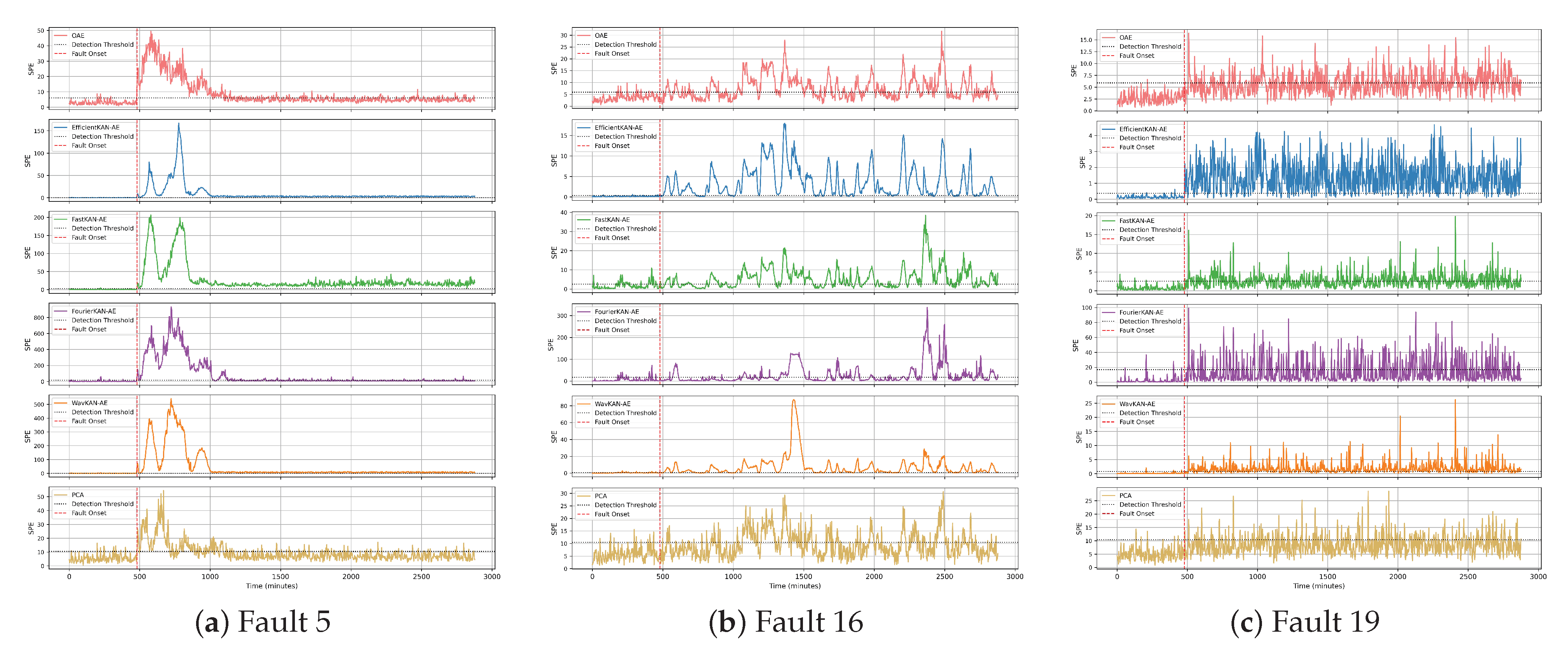
Within the step fault category, all models achieved detection rates above 98%, demonstrating consistent detection of large, steady-state deviations. Fault 5, however, proved considerably more challenging (see Figure 6a). Although the control system restored the measured process variables to their nominal values, the cooling water valve position remained outside the normal operating region. Models that do not capture the coupling between manipulated and controlled variables failed to recognize this deviation, as seen in PCA, OAE, and FourierKAN-AE. In contrast, EfficientKAN-AE, FastKAN-AE, and WavKAN-AE achieved near-perfect detection (98–100%), indicating that their nonlinear parameterization captured subtle correlations between valve position and the system’s thermal balance.

Faults arising from random deviations in process parameters or from sticking valves constitute one of the most challenging categories for process monitoring. Their detectability depends strongly on how the disturbance propagates through the process. When the induced variability drives key measured variables far outside the normal operating region, the fault becomes easy to detect despite the fluctuations in the monitoring index, as observed for faults 12, 14, 17, and 18. In other cases, where the disturbance is partially compensated by control action or results from valve stiction, the monitoring index often fluctuates around or even drops below the detection threshold during the fault window, leading to missed detections as depicted in Figure 6b,c. This behavior reflects the inability of static reconstruction models to capture temporal dependencies and to respond consistently to delayed or fluctuating fault signatures. The limitation is not unique to KAN-AEs but applies broadly to all models that lack explicit temporal dynamics. Incorporating recurrent or sequence-aware architectures, such as RNNs or LSTMs, could mitigate this issue by embedding temporal context into the latent representation. Within the static model class, EfficientKAN-AE consistently outperformed the other architectures, demonstrating greater sensitivity to time-varying disturbances.

4.3. Computational Efficiency

Table 6. Average forward and backward pass durations (mean ± 95% CI) and slowdown ratios for all autoencoder variants on CPU and GPU.

Model (Device)	Fwd. Time [ms]	Fwd. Slowdown	Bwd. Time [ms]	Bwd. Slowdown
OAE (CPU)	0.44 ± 0.04	1.0	0.55 ± 0.04	1.0
OAE (GPU)	0.21 ± 0.01	1.0	0.54 ± 0.02	1.0
EfficientKAN-AE (CPU)	2.90 ± 0.04	6.7	2.05 ± 0.03	3.7
EfficientKAN-AE (GPU)	1.20 ± 0.03	5.6	1.03 ± 0.03	1.9
FastKAN-AE (CPU)	0.97 ± 0.03	2.2	1.25 ± 0.04	2.3
FastKAN-AE (GPU)	0.53 ± 0.01	2.5	0.73 ± 0.01	1.4
FourierKAN-AE (CPU)	1.44 ± 0.04	3.3	1.69 ± 0.04	3.0
FourierKAN-AE (GPU)	0.45 ± 0.01	2.1	0.77 ± 0.04	1.4
WavKAN-AE (CPU)	1.83 ± 0.04	4.2	2.66 ± 0.05	4.8
WavKAN-AE (GPU)	0.64 ± 0.01	3.0	0.86 ± 0.03	1.6

summarizes the average forward and backward pass durations per training batch and slowdown ratios for all autoencoder variants on CPU and GPU. Slowdown ratios indicate the factor by which computation times increase relative to the OAE baseline on the same device. As expected, using a basis expansion to define KAN edge functions (see Appendix A) increases computational cost in KAN-AEs compared with the MLP-based OAE. On the CPU, slowdown ratios range from 2 to 7×, while on the GPU they range from 1.4 to 5.6× depending on the variant. FastKAN-AE and FourierKAN-AE exhibit the lowest overheads (GPU slowdowns < 2.5×), whereas EfficientKAN-AE and WavKAN-AE are notably slower.

Nevertheless, the absolute per-batch times remain modest. Even the slowest variant, EfficientKAN-AE, requires only ≈$1.2\mathrm{ms}$ for a forward pass on GPU, while the fastest models (FastKAN-AE and FourierKAN-AE) complete the same operation in ≈$0.5\mathrm{ms}$. These latencies correspond to processing rates above ${10}^5\mathrm{samples}/\mathrm{s}$, several orders of magnitude faster than the $180\mathrm{s}$ sampling interval of the TEP. Inference speed is therefore not a limiting factor for real-time deployment.

Beyond inference, full retraining is also computationally feasible. With a batch size of $B=256$ and $N={10}^5$ fault-free samples, the slowest model (EfficientKAN-AE) completes an epoch in ≈$0.9\mathrm{s}$ on GPU and ≈$1.9\mathrm{s}$ on CPU, leading to total retraining times of ≈$9\min$ and ≈$19\min$, respectively, for 600 epochs. For comparison, the OAE baseline requires only 3–4 min under identical conditions. Thus, even the most computationally demanding KAN-AE variant is less than a factor of three slower than the OAE, a difference that is negligible in practical retraining scenarios.

The analysis above assumes that hyperparameter tuning has already been completed and that models are retrained using fixed, optimized settings. If extensive hyperparameter searches are included (e.g., 500 configurations via grid or TPE search), the total wall-clock time increases proportionally to the per-epoch cost. Under the same settings ($B=256$, $N={10}^5$), EfficientKAN-AE (GPU) requires approximately $0.87\mathrm{s}$ per epoch, corresponding to ≈$1.45\min$ per trial (100 epochs) or ≈$12\mathrm{h}$ for 500 trials on a single GPU. In contrast, the OAE completes a trial in ≈$0.49\min$, or ≈$4\mathrm{h}$ for 500 trials. While parallelization can reduce overall tuning time, KAN-based architectures remain inherently more computationally demanding during large-scale hyperparameter optimization.

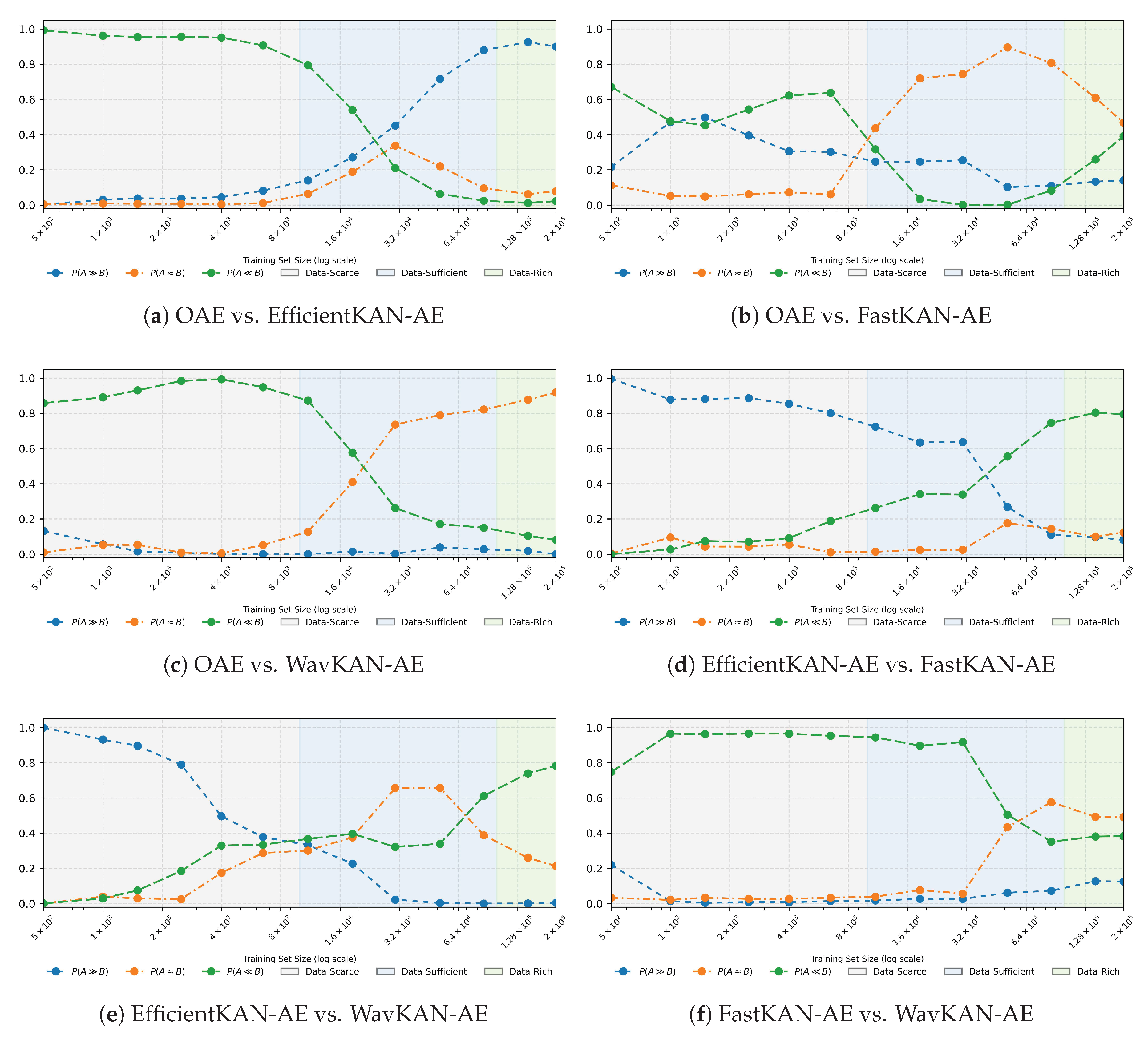
4.4. Bayesian Comparison Across Training Set Sizes

To determine whether observed differences in detection performance among nonlinear methods were statistically meaningful, we applied the Bayesian signed-rank test (Section 3.8). The analysis focused on a subset of challenging faults, where performance differences were most likely to emerge. Faults in which PCA achieved near-perfect detection (FDR $>95\%$, as reported in [5]) and controllable faults, where high FDRs may reflect over-sensitivity rather than genuine detection capability, were excluded. The resulting evaluation set comprised nine faults: Fault 5, 10, 11, 16–21, each treated as an independent comparison unit. For each model pair, we computed the posterior probabilities $P_{\mathrm{left}}$, $P_{\mathrm{rope}}$, and $P_{\mathrm{right}}$, which represent the belief that model A is practically superior to model B, that their performance is equivalent within the ROPE, or that model B is better. These probabilities were tracked across training set sizes to reveal how relative performance evolved as more data became available. The resulting trends complement the mean FDR profiles discussed in Section 4.1, providing a probabilistic basis for model selection as a function of $n_{\mathrm{train}}$.

FourierKAN-AE was omitted from this analysis because of its consistently poor performance across fault types and training set sizes. Including it in pairwise tests would not yield informative distinctions, since posterior comparisons involving clearly dominated models tend to collapse onto the extremes (e.g., $P_{\mathrm{right}}\approx 1$), offering little inferential value.

4.4.1. Orthogonal Autoencoder vs. KAN-Based Autoencoders

As shown in Figure 7a, EfficientKAN-AE demonstrated a clear advantage in the data-scarce regime. For $n_{\mathrm{train}}\le 6500$, the posterior mass lay overwhelmingly in $P_{\mathrm{right}}$ (>0.90), peaking at 0.992 for $n_{\mathrm{train}}=500$. This provides strong evidence that EfficientKAN-AE outperforms OAE when data are limited. However, this advantage diminished steadily as $n_{\mathrm{train}}$ increased. Between 11,000 and 30,000 training samples, the posterior probability shifted toward the ROPE, and eventually to $P_{\mathrm{left}}$, indicating a reversal in relative performance. By $n_{\mathrm{train}}=$ 51,500, OAE was favored with $P_{\mathrm{left}}=0.72$, and this belief strengthened to $P_{\mathrm{left}}=0.93$ by 144,000 training samples. These results highlight EfficientKAN-AE’s strong data efficiency but also its declining competitiveness as more training data became available.

FastKAN-AE showed a more ambiguous performance profile. At smaller $n_{\mathrm{train}}$ values (4000–6500), it held a modest advantage, with $P_{\mathrm{right}}$ peaking at 0.64. Yet, this advantage was never decisive, and the posterior mass shifted rapidly toward the ROPE as $n_{\mathrm{train}}$ increased. Beyond 18,500 samples, practical equivalence dominated the posterior ($P_{\mathrm{rope}}>0.70$), reaching 0.90 at 51,500 training samples. Notably, FastKAN was never overtaken by OAE, as $P_{\mathrm{left}}$ remained consistently low, but it also failed to establish a clear lead, with $P_{\mathrm{right}}$ never exceeding 0.70 (see Figure 7b). This pattern indicates that FastKAN-AE converged toward performance parity with OAE across most data regimes, offering only marginal gains in detection capability.

WavKAN-AE delivered the most robust early-stage performance. For $n_{\mathrm{train}}\le 6500$, $P_{\mathrm{right}}$ exceeded 0.94, peaking at 0.993 for $n_{\mathrm{train}}=4000$. As $n_{\mathrm{train}}$ increased, the posterior mass migrated toward the ROPE, reflecting a transition toward practical equivalence rather than a reversal in relative performance (Figure 7c). By 30,500 training samples, ROPE accounted for 74% of the posterior mass, rising to 92% at 200,000 samples. Importantly, $P_{\mathrm{left}}$ remained near zero throughout, showing that OAE never overtook WavKAN-AE. This underscores WavKAN-AE’s robustness in data-scarce regimes and its capacity to maintain competitive performance as data availability increased, without the degradation observed for EfficientKAN-AE.

Collectively, these results reveal distinct generalization behaviors across KAN-based architectures. EfficientKAN-AE excelled when data were limited but was ultimately surpassed as the training set grew. FastKAN-AE provided modest gains in low-data regimes and converged toward equivalence with OAE. WavKAN-AE achieved the strongest early-stage performance and maintained competitiveness across all data regimes. These findings emphasize the importance of aligning model choice with data availability: EfficientKAN-AE is preferable under data scarcity, WavKAN-AE offers stable performance across conditions, and OAE remains a competitive option in data-rich scenarios.

4.4.2. Pairwise Comparisons Among KAN-Based Autoencoders

In the data-scarce regime, EfficientKAN-AE consistently outperformed the other KAN-AEs by a substantial margin. The posterior probability mass favoring EfficientKAN-AE exceeded 0.85 in all pairwise comparisons, reaching $P_{\mathrm{right}}=0.996$ against FastKAN-AE (Figure 7d) and $P_{\mathrm{right}}=0.999$ against WavKAN-AE (Figure 7e). Within the same regime, WavKAN-AE maintained a moderate yet consistent advantage over FastKAN-AE, with posterior mass above 0.74 (Figure 7f), although this margin was considerably smaller than that of EfficientKAN-AE.

As the training set entered the data-sufficient regime, WavKAN-AE emerged as the most robust model. It outperformed FastKAN-AE throughout this range, with $P_{\mathrm{right}}>0.90$ in every relevant comparison. Against EfficientKAN-AE, the posterior distribution shifted more gradually: a broad region of practical equivalence initially dominated, but belief in WavKAN-AE’s superior performance strengthened with additional data and eventually overtook EfficientKAN-AE midway through the regime.

In the data-rich regime, both WavKAN-AE and FastKAN-AE surpassed EfficientKAN-AE. Posterior mass favoring FastKAN-AE increased steadily, reaching 0.80 at the upper end of the regime, while WavKAN-AE continued to outperform EfficientKAN-AE with $P_{\mathrm{right}}=0.78$. However, FastKAN-AE never overtook WavKAN-AE since its posterior advantage grew only slightly with data and remained below 0.40 throughout. In large-data comparisons between WavKAN-AE and FastKAN-AE, the posterior mass concentrated within the ROPE, indicating practical equivalence.

4.5. Limitations and Future Work

This study has some limitations worth noting. The evaluation was conducted exclusively on the Tennessee Eastman Process, which, although widely used as a benchmark, does not fully capture the variability and operational complexity of real industrial systems. Extending the analysis to other dynamic benchmarks or real plant data would provide stronger empirical support for the observed trends.

A second limitation is that the current framework does not explicitly account for temporal dependencies among process variables. The autoencoders were trained on static inputs, which capture local correlations but not the time-dependent patterns characteristic of normal operation. Incorporating explicit sequence modeling through recurrent, convolutional, or attention-based architectures could influence the scaling behavior of fault detection performance and potentially modify the relative trends observed between KAN- and MLP-based models. Evaluating such temporal extensions within the same comparative framework would clarify whether the data-efficiency advantages of KANs persist when temporal structure is modeled explicitly.

Finally, hybrid architectures combining KAN and MLP layers were not explored. The present analysis focused exclusively on fully KAN-based or fully MLP-based autoencoders, leaving open the question of whether hybrid designs can better balance data efficiency and computational cost. Architectures in which KAN layers serve as nonlinear feature expansions, or where the encoder employs KAN layers while the decoder remains an MLP, could retain the representational richness of KANs while mitigating their computational overhead. Future comparative studies should examine whether such hybrid configurations provide a more practical trade-off between accuracy, data efficiency and computational cost for industrial fault detection.

5. Conclusions

This study evaluated Kolmogorov–Arnold Autoencoders (KAN-AEs) for unsupervised fault detection in chemical process systems. The results demonstrate that KAN-AEs outperform conventional MLP-based autoencoders under limited data availability but provide no significant advantage in data-rich regimes. Model performance also depended on the choice of basis family in the univariate edge functions: local bases (B-splines, wavelets) were more effective than global ones (Fourier modes) in capturing process variability. Overall, KAN-AEs offer a compact and data-efficient alternative for industrial monitoring applications where historical fault-free data are limited or costly to obtain.