Article

Trajectory Tracking Control of Hydraulic Flexible Manipulators Based on Adaptive Robust Model Predictive Control

1
School of Intelligent Control, Changzhou Vocational Institute of Industry Technology, Changzhou 213164, China
2
School of Electronic and Optical Engineering, Nanjing University of Science and Technology, Nanjing 210094, China
3
College of Communication Engineering, Jilin University, Changchun 130022, China
*
Author to whom correspondence should be addressed.
Processes 2025, 13(11), 3638; https://doi.org/10.3390/pr13113638
Submission received: 22 September 2025 / Revised: 5 November 2025 / Accepted: 6 November 2025 / Published: 10 November 2025
(This article belongs to the Special Issue Advances in Green Process Systems Engineering)

Abstract

Aiming at the trajectory tracking control problem caused by the coupling of strong nonlinearity, parameter uncertainty and unknown disturbances in rigid robotic arms, this paper proposes an adaptive robust model predictive control (APRMPC) scheme. This study aims to fill the gap in the existing literature by proposing a dedicated control framework capable of simultaneously and effectively handling parameter uncertainty, unmodeled dynamics, and external disturbances, while ensuring constraint satisfaction. Firstly, a dynamic model of a three-degree-of-freedom robotic arm was established based on the Lagrange equation; secondly, this paper designs a deep integration mechanism of adaptive law and robust predictive control: by designing a parameter adaptive algorithm to estimate the system uncertainty online and feedforward compensate it to the predictive model, the impact of model mismatch is significantly reduced; meanwhile, for the estimated residuals and unknown disturbances, feedback gain was introduced and the control input was designed based on the robust invariant set theory, achieving unified parameter identification, disturbance suppression and rolling optimization within a single framework. This paper strictly proves the feasibility and stability of the control scheme. Finally, the simulation experiments based on MATLAB show that, compared with the traditional MPC and PID methods, the APRMPC algorithm can achieve higher accuracy and stronger robustness in trajectory tracking under various working conditions, effectively resolving the inherent contradiction between the weak robustness of the traditional MPC and the large buffering of sliding mode control, and verifying the value of the proposed scheme in filling the gap in related literature.

1. Introduction

In recent years, with the rapid advancement of robotics technology, manipulators have found increasingly widespread application in fields such as industrial assembly, precision medicine, aerospace, and modern agriculture [1,2,3]. The increasing complexity of tasks and requirements for environmental adaptability have imposed stricter requirements on the accuracy and robustness of manipulator trajectory tracking. However, manipulator systems are inherently highly nonlinear, strongly coupled, and possess complex dynamic characteristics. Furthermore, during actual operation, they are often subjected to multiple uncertainties, including model parameter perturbations, unmodeled dynamics, and external unknown disturbances [4], which significantly increase the difficulty of high-precision control. This is particularly evident in hydraulically driven flexible manipulators, where the coupling between structural flexibility and hydraulic dynamics further exacerbates system uncertainties and control challenges. When a manipulator operates in an environment with external disturbances or time-varying conditions, its tracking performance often degrades substantially, potentially even leading to control failure. Therefore, developing high-precision control strategies capable of suppressing model uncertainties, overcoming external disturbances, and ensuring stable tracking performance is of significant theoretical importance and engineering application value.
To achieve high-precision trajectory tracking control for manipulators, researchers worldwide have proposed various control strategies, making remarkable progress at both theoretical and application levels. Traditional control methods such as proportional–integral–differential (PID) control, model predictive control (MPC), sliding mode control (SMC), as well as intelligent control methods based on neural networks and fuzzy logic, have all demonstrated effectiveness in manipulator trajectory tracking [5,6,7]. Among these, PID control remains widely used in many industrial applications due to its simple structure, intuitive parameter tuning, and high practical utility. For example, Yin et al. [8] proposed a PID-type iterative learning control method based on a time-varying sliding surface, achieving precise trajectory tracking for a two-degree-of-freedom manipulator and stabilizing the tracking error on a predefined sliding surface. Loucif et al. [9] optimized PID controller parameters using the whale optimization algorithm. Through comparisons with particle swarm optimization and grey wolf optimization methods, they validated the superiority of their strategy in reducing trajectory errors and shortening settling time. However, PID controllers rely on linear time-invariant models and struggle to effectively handle systems with high-order, nonlinear, and strongly coupled characteristics such as rigid manipulators. Their fixed parameters are inadequate for adapting to changing operating points and external disturbances, exhibiting significant limitations in robustness.
To enhance the ability to counteract uncertainties, SMC has been widely applied to manipulator control due to its invariance to matched disturbances and its ability to drive the system state to converge to the sliding surface within finite time. Xue et al. [10] developed a manipulator system based on SMC-PID control for high-quality tender tea bud picking, improving response speed and stability while ensuring picking accuracy. Mobayen et al. [11] proposed a robust adaptive super-twisting global nonlinear sliding mode strategy, enabling the manipulator to converge within finite time even in the presence of uncertainties and external disturbances, significantly enhancing system robustness. Chen et al. [12] designed a nonsingular fast integral terminal sliding mode controller, which avoids singularity issues by introducing an integral term while enhancing disturbance rejection capability. This approach reduces steady-state error while improving convergence speed. Nevertheless, the inherent chattering phenomenon in sliding mode control hinders its broader application in rigid manipulators. Such systems inherently exhibit high-frequency response characteristics, and chattering not only causes drastic variations in control signals but may also excite unmodeled dynamics, potentially leading to system instability. Therefore, chattering must be effectively suppressed in practical applications.
To address system constraints and achieve optimal control, MPC has received significant attention due to its ability to explicitly handle state and input constraints, incorporate rolling optimization and feedback correction mechanisms, and provide multi-step prediction capabilities [13]. For instance, Wang [14] proposed an MPC-based obstacle avoidance control framework for a three-degree-of-freedom manipulator. By integrating forward/inverse kinematics with a discrete linear state-space model, smooth and collision-free trajectory planning was achieved. Simulation results demonstrated that the controller effectively balanced prediction accuracy, constraint satisfaction, and dynamic response. Yan et al. [15] introduced a data-driven neurodynamic model predictive control algorithm that combined an MPC architecture, a neurodynamic solver, and a discrete Jacobian matrix update law. This approach effectively predicted the future output of redundant manipulators and constructed a trajectory tracking MPC strategy that outperformed traditional methods. However, the performance of conventional MPC depends heavily on model accuracy. When faced with unmodeled dynamics, parameter perturbations, and external disturbances inherent in rigid manipulators, its robustness often proves insufficient. To reduce reliance on precise models, numerous intelligent control methods have been introduced into this field. Leveraging their powerful nonlinear approximation and fuzzy reasoning capabilities, neural networks and fuzzy control have been widely used for online identification of system uncertainties or adaptive adjustment of controller parameters. For example, Muthusamy et al. [16] designed a fuzzy neural network controller based on a bidirectional brain emotional learning algorithm to address uncertainties arising from stiffness and load variations. Simulations showed that this controller exhibited better adaptability and tracking performance than traditional PID under varying stiffness and load conditions. Liu et al. [17] constructed an adaptive fuzzy neural network to approximate model uncertainties and combined it with an adaptive disturbance observer to estimate unknown disturbances, thereby effectively enhancing system robustness. Simulation results validated the effectiveness of this strategy. Although such methods improve system performance to some extent, the stability proofs for their controllers are often complex and heavily reliant on expert experience or extensive training data.
Adaptive control (APC) provides an effective means to address time-varying system characteristics through the online adjustment of controller parameters or real-time estimation of unknown system parameters. To actively suppress lumped uncertainties while ensuring stability and constraint satisfaction, composite control architectures integrating the parameter identification capability of APC, the disturbance rejection performance of robust control, and the constraint optimization ability of MPC have become an important research direction for complex systems. In recent years, adaptive robust model predictive control has attracted widespread attention and achieved significant progress. For example, Köhler et al. [18] proposed a tube-based robust adaptive MPC framework to handle parameter uncertainties and additive disturbances in nonlinear systems. Pereida et al. [19] developed an algorithm combining robust MPC and discrete-time adaptive control, enabling rapid and accurate stabilization of systems under model uncertainty. Xu et al. [20] proposed a novel discrete-time extended state observer-based model-free adaptive SMC scheme for uncertain nonlinear systems, which achieves improved tracking accuracy and robustness without relying on mathematical models by combining dynamic linearization, chattering suppression, and genetic algorithm optimization. Building on this, Wei et al. [21] further proposed a discrete-time integral terminal sliding mode predictive control method for high-precision posture tracking of hydraulic flexible manipulators. This method enhances performance by combining predictive control with an adaptive sliding mode strategy to reduce chattering and improve tracking accuracy. However, applying such methods to hydraulically driven manipulator systems with significant structural flexibility and strong coupling characteristics still faces challenges related to real-time performance, computational complexity, and chattering suppression.
In summary, although control methods such as model predictive control, adaptive control, and robust control have achieved certain results in manipulator trajectory tracking, they still face limitations when dealing with compound uncertainties—including strong nonlinearities, time-varying parameters, and unknown disturbances—in rigid manipulator systems. Single-method control strategies often suffer from issues such as insufficient stability, difficulty in strictly satisfying constraints, or limited disturbance rejection capability. To address the aforementioned challenges, this paper proposes a novel APRMPC framework. It is designed to integrate the online parameter identification capability of adaptive control, the disturbance rejection capabilities of robust control, and the constraint optimization performance of model predictive control, thereby achieving high-precision trajectory tracking while ensuring system stability. The main contributions of this work include the following: establishing a dynamic model of a three-degree-of-freedom rigid manipulator; designing an adaptive parameter update law based on Lyapunov stability theory; developing an APRMPC controller with disturbance rejection capability and rigorously proving its closed-loop stability; and finally, validating the superiority of the proposed method in tracking accuracy, robustness, and constraint compliance through comparative simulation experiments. This study provides a theoretically sound and practically valuable solution for the control of complex electromechanical–hydraulic coupled systems, contributing positively to the advancement of control technologies in high-end equipment and precision operation applications. The contributions of this article are as follows:
(1) An innovative adaptive robust model predictive controller suitable for rigid robotic arms was designed. The APC can quickly estimate the uncertain model parameters caused by hydraulic nonlinearity, parameter uncertainty and flexible vibration online. RMPC conducts rolling optimization based on the compensated nominal model and actively suppresses interference by using the robust invariant set to ensure that the system fully satisfies the constraints throughout the process. This design, in terms of mechanism, simultaneously combines the accuracy of online estimation of model parameters and the reliability of feedback robustness, effectively overcoming the problems of weak robustness and large buffering in sliding mode control of traditional MPC.
(2) A three-degree-of-freedom (3-DOF) robotic arm prediction model was established, providing a high-precision prediction foundation for MPC. Through comparative experiments with PID and traditional MPC in multiple scenarios, the significant advantages of the proposed method in tracking accuracy and anti-interference ability have been fully verified, providing a practical basis for engineering applications.

2. Modeling

2.1. Dynamic Model of the Three-Degree-of-Freedom Manipulator

This study employs a three-degree-of-freedom (3-DOF) manipulator as the control object. As a fundamental subject in robotics research, the 3-DOF manipulator is widely used in industrial, medical, and service robot applications due to its simple structure, low cost, and capability to perform basic spatial motions. Figure 1a shows the structure of the 3-DOF manipulator, which typically consists of three rotary joints: the shoulder joint allows horizontal rotation, and the elbow joint enables vertical rotation, thereby facilitating complex motions in three-dimensional space. l 1 , l 2 , l 3 denote the lengths of each link, and m 1 , m 2 , m 3 represent the masses of each link and the corresponding joint driving units. The control of the manipulator is generally executed by a microcontroller or computer, which drives motors to regulate the motion of each joint.
As shown in Figure 1b, a schematic diagram of the 3-DOF manipulator structure is presented. To characterize the kinematic properties of the 3-DOF manipulator, a rotating coordinate system XOY and a body-fixed follow-up coordinate system XOZ attached to the manipulator are established. Assuming that the masses of the three links and the driving units are lumped at the rotational centers of each joint, points φ 1 , φ 2 , φ 3 represent the angular displacements of the respective joints. Using Lagrange’s equation method, the following dynamic model of the system can be derived:
M φ φ ¨ + C φ , φ ˙ φ ˙ + G φ = τ + ω
where M φ represents the inertial mass matrix of the manipulator; C φ , φ ˙ denotes the centrifugal and Coriolis force vector; G φ corresponds to the gravitational force vector matrix; τ indicates the control input of the manipulator system; and ω represents the uncertainty disturbance. The specific parameters of the system are defined as follows:
φ = φ 1 φ 2 φ 3 T φ ˙ = φ ˙ 1 φ ˙ 2 φ ˙ 3 T φ ¨ = φ ¨ 1 φ ¨ 2 φ ¨ 3 T τ = τ 1 τ 2 τ 3 T ω = ω 1 , ω 2 , ω 3 T
where φ 1 , φ 2 , φ 3 represent the angular displacements of Joint 1, Joint 2, and Joint 3, respectively; φ ˙ 1 , φ ˙ 2 , φ ˙ 3 denote the angular velocities of Joint 1, Joint 2, and Joint 3, respectively; φ ¨ 1 , φ ¨ 2 , φ ¨ 3 indicate the angular accelerations of Joint 1, Joint 2, and Joint 3, respectively; τ 1 , τ 2 , τ 3 correspond to the driving torques of Joint 1, Joint 2, and Joint 3, respectively; and ω 1 , ω 2 , ω 3 represent the uncertain disturbances affecting Joint 1, Joint 2, and Joint 3, respectively.

2.2. Discrete State-Space Equation of the Three-Degree-of-Freedom Manipulator

The nonlinear dynamic model of the 3-DOF manipulator can be derived from Equation (1). In this paper, the state vector of the system is defined as x = [ φ φ ˙ ] , which consists of the angular displacements and angular velocities of each joint of the manipulator, and the control input is defined as u = τ , representing the system control torques. The state-space equation of the manipulator control system can be expressed as
x ˙ = f ( x , u ) f ( x , u ) = φ ˙ M 1 ( φ ) τ + ω C ( φ , φ ˙ ) φ ˙ G ( φ )
To facilitate subsequent controller design, Equation (2) is linearized using the Jacobian method. The Jacobian submatrices of each component’s derivative function f x , u are given as follows:
A l = f 1 / x 1 f 1 / x 2 f 1 / x 6 f 2 / x 1 f 2 / x 2 f 2 / x 6 f 6 / x 1 f 6 / x 2 f 6 / x 6
B l = f 1 / u 1 f 1 / u 2 f 1 / u 3 f 2 / u 1 f 2 / u 2 f 2 / u 3 f 6 / u 1 f 6 / u 2 f 6 / u 3
At an equilibrium point, the system states satisfy x = x r , x ˙ = x ˙ r , and the control input is u = u r . It is assumed that at the equilibrium point, the control vector is u e , the state vector is x e , and the time derivative is x ˙ e . Linearizing the Jacobian matrices given in Equations (4) and (5) at the equilibrium point yields
x ˙ = A l x + B l u + ω
In practical control of the manipulator, state information is typically transmitted through discrete sampling. Therefore, a zero-order holder with a sampling period T s is used to discretize the system. The continuous state-space equation Equation (6) is transformed into a discrete form, and a disturbance term W t is added. The resulting discrete state-space equation of the manipulator is expressed as
x t + 1 = Ax t + Bu t + W t
where A = e A l T s ; B = 0 T s e A l t B l dt ; W t = w 1 t w 2 t w 3 t 0 0 0 T .

3. Adaptive Parameter Estimation

3.1. Adaptive Update Law for Model Parameters

During actual operation, the manipulator is susceptible to factors such as friction and mechanical wear, leading to uncertainties in the model parameters A and B . To address this issue, an adaptive control method capable of identifying model parameters online is designed in this section, thereby providing a foundation for the subsequent manipulator controller design.
The manipulator dynamic model without the disturbance parameter W t is rewritten into the discretized system model and the estimation model, respectively, as
x ¯ k + 1 = A x ¯ k + B u ¯ k
x ¯ ^ k + 1 = A ^ k x ¯ k + B ^ k u ¯ k
where A ^ k , B ^ k denote the estimated value of A and B , respectively, representing the actual parameter values of the 3-DOF manipulator model. Θ k A , B , then Θ ^ k A ^ k , B ^ k ; x ¯ ^ k denotes the estimated value of the system state x ¯ k . Furthermore, models (8) and (9) can be expressed in a compact form as
x ¯ k + 1 = Θ k Φ ¯ k
x ¯ ^ k + 1 = Θ ^ k Φ ¯ k
where Φ ¯ k = x ¯ T k , u ¯ T k T . Based on Equations (10) and (11), we obtain
x k + 1 = Θ k Φ ¯ k
where x k + 1 x ¯ k + 1 x ¯ ^ k + 1 is the system state error, and Θ k Θ k Θ ^ k is the system model error. To minimize the system state error, a cost function for estimating the system error is designed as follows:
Θ ^ k = arg min Θ ^ k H x k + 1 H x k + 1 = x k + 1 T x k + 1
 Definition 1. 
Let Θ = θ i j m × n R m × n , x R m , y R n . Both x and y are column vectors. Define the partial derivative of the multivariate function f x , y , Θ = x T Θ y with respect to the matrix Θ as
f x , y , Θ Θ = y x T
 Assumption A1. 
For the estimated value Θ ^ k A ^ k , B ^ k of the uncertain model parameters, there exists a supremum Θ ¯ such that Θ ^ Θ ¯ .
According to Definition 1, the partial derivative of Equation (13) is calculated as
H = H Θ ^ = Θ ^ x ¯ ( k + 1 ) Θ ^ ( k ) Φ ¯ ( k ) T x ¯ ( k + 1 ) Θ ^ ( k ) Φ ¯ ( k ) = Θ ^ x ¯ T ( k + 1 ) x ¯ ( k + 1 ) 2 x ¯ T ( k + 1 ) Θ ^ ( k ) Φ ¯ ( k ) + Φ ¯ T ( k ) Θ ^ T ( k ) Θ ^ ( k ) Φ ¯ ( k ) = 2 Φ ¯ ( k ) x ¯ ( k + 1 ) Θ ^ ( k ) Φ ¯ ( k ) T = 2 Φ ¯ ( k ) x T ( k + 1 )
Therefore, the adaptive update law for the model parameters using the negative gradient descent method is given by
Θ ^ k + 1 = Θ ^ k λ 2 H T = Θ ^ k + λ x k + 1 Φ ¯ T k
where λ represent the learning rate that influences the update rate of the system.

3.2. Stability Analysis

 Theorem 1. 
For the 3-DOF manipulator model (9) with uncertain parameters, if there exists a feasible control input u ¯ k , then according to the adaptive update law (16), the model parameter estimation error Θ ^ k is bounded, and the estimated state error x ^ k is asymptotically stable.
Φ ¯ T k Φ ¯ k 2 α λ
where 0 < α < 2 and λ > 0 are adjustable parameters.
 Proof. 
Consider the following Lyapunov function candidate: V k = tr Θ T k Θ k , where tr · denotes the trace of a matrix. Then, V k + 1 can be expressed as
V ( k + 1 ) = tr Θ T ( k + 1 ) Θ ( k + 1 ) = tr Θ T ( k + 1 ) Θ ( k + 1 ) 2 Θ T ( k + 1 ) Θ ^ ( k + 1 ) + Θ ^ T ( k + 1 ) Θ ^ ( k + 1 )
Using properties of the matrix trace, Equation (18) can be further expressed as
V ( k + 1 ) = tr Θ T ( k ) Θ ( k ) 2 tr Θ T ( k ) Θ ^ ( k ) λ 2 H T + tr Θ ^ T ( k ) Θ ^ ( k ) λ Θ ^ T ( k ) H T + λ 2 4 H H T = V ( k ) + tr λ Θ T ( k ) H T + λ 2 4 H H T
From Equation (15), it can be derived that
tr λ Θ T ( k ) H T + λ 2 4 H H T = λ tr 2 Θ T ( k ) x ( k + 1 ) Φ ¯ T ( k ) + λ Φ ¯ ( k ) x T ( k + 1 ) x ( k + 1 ) Φ ¯ T ( k ) = λ 2 + λ Φ ¯ T ( k ) Φ ¯ ( k ) x T ( k + 1 ) x ( k + 1 )
According to Condition (17), it can be concluded that 2 + λ Φ ¯ T ( k ) Φ ¯ ( k ) α . Therefore, it follows that
V ( k + 1 ) V ( k ) λ α x T ( k + 1 ) x ( k + 1 )
In summary, V ( k ) is a monotonically decreasing function and V ( k ) > 0 ; hence, lim k V ( k ) exists. This implies that the model parameter estimation error Θ ( k ) is bounded.
From Equation (21), we have
V ( 1 ) V ( 0 ) λ α x T ( 1 ) x ( 1 ) V ( 2 ) V ( 1 ) λ α x T ( 2 ) x ( 2 ) V ( k + 1 ) V ( k ) λ α x T ( k + 1 ) x ( k + 1 )
Therefore, clearly V ( k + 1 ) V ( 0 ) λ α j = 1 k + 1 x T ( j ) x ( j ) ; then, the following can be obtained:
lim k λ α j = 1 k + 1 x T ( j ) x ( j ) V ( 0 ) lim k V ( k + 1 )
Moreover, since lim k V ( k ) exists, j = 1 k + 1 x T ( j ) x ( j ) converges. Hence, the estimated state error x ( k ) is asymptotically stable, and lim k x ( k ) = 0 . □

4. Adaptive Robust Model Predictive Controller

4.1. Design of Adaptive Robust Predictive Controller

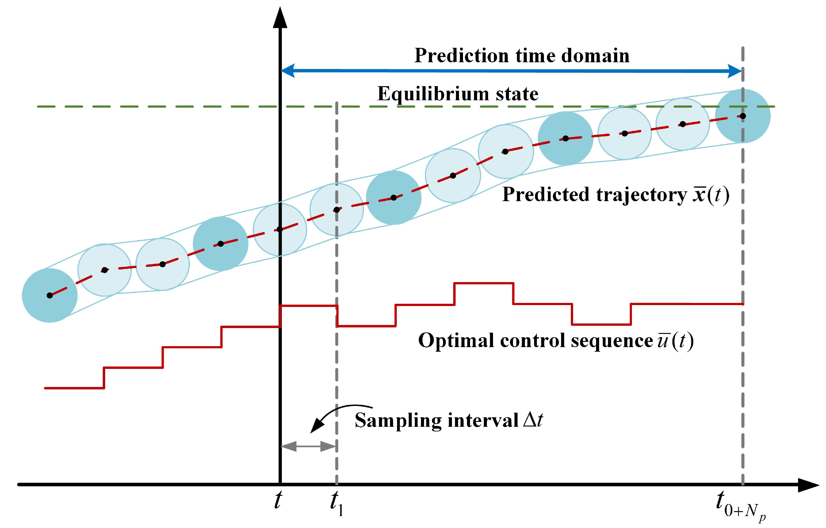
When the manipulator system is subjected to disturbances, the feasibility and stability of the controller cannot be guaranteed. Ignoring system uncertainties might serve as an idealized solution, but it can compromise control performance and lead to system instability. Therefore, this section designs a robust model predictive control strategy based on a feedback approach to achieve precise and stable control of the manipulator. As shown in Figure 2, a timing diagram of the robust model predictive control illustrates the concept: predictive control actions drive the manipulator’s operating state toward equilibrium, and despite disturbances, the feedback control law ensures the system state at each discrete time step remains within an allowable error range [22,23,24].
First, the estimated system model derived in the previous section is expressed as follows:
x k + 1 = A ^ k x k + B ^ k u k
During the operation of the manipulator, in addition to disturbances affecting the model parameters, the system may also be subject to additional indescribable unknown disturbances. Therefore, the model is further represented as
x k + 1 = A ^ k x k + B ^ k u k + W k
where W ( t ) = w 1 ( t ) w 2 ( t ) w 3 ( t ) 0 0 0 T W = W ( k ) R 6 : W ( k ) ω ¯ is a bounded disturbance.
To distinguish the impact of additional disturbances on the system, model (25) is decomposed into a nominal model (26) and a disturbance model (27):
x ¯ k + 1 = A ^ k x ¯ k + B ^ k u ¯ k
x ˜ k + 1 = A ^ k x ˜ k + B ^ k u ˜ k + W k
where x ¯ k and x ˜ k represent the nominal state and disturbance state at time k, respectively; u ¯ k and u ˜ k denote the nominal control input and disturbance control input at time k, respectively; and x ¯ k + x ˜ k = x k , u ¯ k + u ˜ k = u k .
 Assumption A2. 
For the nominal model (26), given positive definite symmetric matrices Q and R, there exists a constant α > 0 , a positive definite symmetric matrix H and a local state feedback control law K x ¯ U ¯ , such that for any terminal state x , the following condition holds: Ω H , α : = x X f : x T Hx α , where the terminal state matrix H satisfies
A ^ + B ^ K T H A ^ + B ^ K H + Q + R K T K 0 .
For the 3-DOF manipulator control system with additive disturbances described above, the robust model predictive control (RMPC) method is employed for controller design [25]. First, based on Assumption A1, the control problem for the manipulator is formulated using the nominal model (26) as follows:
min u ¯ · k J x ¯ · k , u ¯ · k = j = 0 N p 1 x ¯ k + j k x ¯ r k + j k Q 2 + u ¯ k + j k R 2
+ x ¯ k + N p k x ¯ r k + N p k H 2
s . t . x ¯ k + j + 1 k = A ^ k x ¯ k + j k + B ^ k u ¯ k + j k
x ¯ k + j k X ¯ X X ˜ , j = 1 , , N p 1 ,
u ¯ k + j k U ¯ U U ˜ , j = 0 , , N p 1 ,
x ¯ k + N p k X ¯ f ,
Φ ¯ T k Φ ¯ k 2 α λ
where X ¯ and X ˜ denote the nominal state constraint set and the disturbance state constraint set, respectively; U ¯ and U ˜ represent the nominal control constraint set and the disturbance control constraint set, respectively. To characterize the disturbance control component u ˜ k , a feedback control gain K f is introduced such that U ˜ K f X ˜ , X ¯ f denotes the terminal constraint set, ensuring that the predicted terminal state lies within the terminal invariant set; in Equation (33), Φ ¯ k = x ¯ T k , u ¯ T k T is the constraint condition that ensures the feasibility of the estimated parameters of the system.
By solving the optimal control problem (28) for the manipulator system at time k, the optimal control sequence u ¯ · k = u ¯ k + j k : j = 0 , 1 , , N p 1 and the predicted state trajectory x ¯ · k = x ¯ k + j k : j = 0 , 1 , , N p can be obtained. For the model predictive controller, the nominal optimal control input is u ¯ k k ; however, due to the presence of disturbances, the actual control input computed by the robust model predictive controller is designed as follows:
u k = u ¯ k k + K f x ˜ k
Since external uncertain disturbances directly affect the angular velocity state variables, the feedback control gain K f = 0 0 0 k 1 k 2 k 3 is designed to compensate for their effect. The RMPC algorithm compensates for angular velocity disturbances via the feedback control defined in Equation (34).
The adaptive robust model predictive controller designed in this section consists of two main components: an adaptive parameter estimation mechanism and a robust predictive controller. The block diagram of the APRMPC algorithm structure is presented in Figure 3.

4.2. Stability Analysis

 Theorem 2. 
If at time k = k d , the optimal control problem J x ¯ · k , u ¯ · k admits a feasible solution, then
(1) For any time k > k d , the optimal control problem remains feasible;
(2) The closed-loop system is stable, and the system state converges to a terminal invariant set Ω near the equilibrium point.
 Proof. 
(1) Suppose at time k, the optimal control problem J x ¯ · k , u ¯ · k yields the optimal control sequence
u ¯ · k = u ¯ k + j k : j = 0 , 1 , , N p 1
and the corresponding optimal state sequence
x ¯ · k = x ¯ k + j k : j = 0 , 1 , , N p
Similarly, at time k + 1 , the optimal control J x ¯ · k + 1 , u ¯ · k + 1 sequence is given by
u ¯ ( · k + 1 ) = u ¯ ( k + 1 + j k + 1 ) : j = 0 , 1 , , N p 1 = u ¯ ( k + 1 k + 1 ) , u ¯ ( k + 2 k + 1 ) , , u ¯ ( k + N p 1 k + 1 ) , u ¯ ( k + N p k + 1 ) = u ¯ ( k + 1 k ) , u ¯ ( k + 2 k ) , , u ¯ ( k + N p 1 k ) , K x ¯ ( k + N p k )
From Assumption A2, x ¯ k + N p k Ω and u ¯ k + N p k = K x ¯ k + N p k U ¯ , it follows that
x ¯ k + N p + 1 k + 1 = A ^ x ¯ k + N p k + 1 + B ^ u ¯ k + N p k + 1 = A ^ + B ^ K x ¯ k + N p k
Thus, at time k + 1 , the corresponding state sequence is
x ¯ ( · k + 1 ) = x ¯ ( k + 1 + j k + 1 ) : j = 0 , 1 , , N p = x ¯ ( k + 1 k + 1 ) , x ¯ ( k + 2 k + 1 ) , , x ¯ ( k + N p k + 1 ) , x ¯ ( k + N p + 1 k + 1 ) = x ¯ ( k + 1 k ) , x ¯ ( k + 2 k ) , , x ¯ ( k + N p k ) , ( A ^ + B ^ K ) x ¯ ( k + N p k )
Therefore, from A ^ + B ^ K x ¯ k + N p k Ω , it follows that
x ¯ k + N p + 1 k + 1 = A ^ + B ^ K x ¯ k + N p k X ¯ f X ¯
Hence, the optimal control problem is feasible at time k + 1 . Since it is feasible at time k = 0 , it remains feasible for all k > 0 .
(2) From Equation (1), the problem is feasible for all k > 0 . From Equation (28), the objective function value corresponding to time k is
J x ¯ ( · k ) , u ¯ ( · k ) = j = 0 N p 1 x ¯ ( k + j k ) x ¯ r ( k + j k ) Q 2 + u ¯ ( k + j k ) R 2 + x ¯ ( k + N p k ) x ¯ r ( k + N p k ) H 2
Substituting (37) and (39) into (28), the objective function value at time k + 1 is
J x ¯ ( · k + 1 ) , u ¯ ( · k + 1 ) = j = 0 N p 1 [ x ¯ ( k + j + 1 k + 1 ) x ¯ r ( k + j + 1 k + 1 ) Q 2 + u ¯ ( k + j + 1 k + 1 ) R 2 ] + x ¯ ( k + N p + 1 k + 1 ) x ¯ r ( k + N p + 1 k + 1 ) H 2
Using Equation (40), Equation (42) can be rewritten as
J x ¯ ( · k + 1 ) , u ¯ ( · k + 1 ) = j = 0 N p 2 x ¯ ( k + j + 1 k ) x ¯ r ( k + j + 1 k ) Q 2 + u ¯ ( k + j + 1 k ) R 2 + x ¯ ( k + N p k ) x ¯ r ( k + N p k ) Q 2 + K x ¯ ( k + N p k ) R 2 + ( A ^ + B ^ K ) x ¯ ( k + N p k ) x ¯ r ( k + N p k ) H 2
From Equation (41), it follows that
J x ¯ ( · k + 1 ) , u ¯ ( · k + 1 ) = J x ¯ ( · k ) , u ¯ ( · k ) x ¯ ( k k ) x ¯ r ( k k ) Q 2 u ¯ ( k k ) R 2 + x ¯ ( k + N p k ) x ¯ r ( k + N p k ) Q + K T R K + ( A ^ + B ^ K ) T H ( A ^ + B ^ K ) 2
It can be inferred that A ^ + B ^ K T H A ^ + B ^ K H + Q + R K T K 0 , and from Assumption A2, it follows that
J x ¯ · k + 1 , u ¯ · k + 1 J x ¯ · k , u ¯ · k
It is evident that when k > 0 , J x ¯ · k , u ¯ · k 0 , the objective function is monotonically bounded and decreasing, the closed-loop system is stable, and the system state tends towards the terminal constraint region Ω near the equilibrium point. □

5. Simulation Experiments

5.1. Simulation Parameter Settings

To comprehensively validate the performance and control effectiveness of the proposed APRMPC algorithm in manipulator trajectory tracking tasks, simulations of a 3-DOF manipulator’s motion process were conducted using MATLAB R2022b. The model information is as follows:
M φ φ ¨ 1 φ ¨ 2 φ ¨ 3 + C φ , φ ˙ φ ˙ 1 φ ˙ 2 φ ˙ 3 + G φ = τ 1 τ 2 τ 3 + ω 1 ω 2 ω 3
The parameters of each matrix in the model are specified below:
M φ = M 11 M 12 M 13 M 21 M 22 M 23 M 31 M 32 M 33 , M i j = k = max i , j 3 m k r c k T φ i r c k φ j + I k ϕ k T φ ˙ i ϕ k φ ˙ j
C φ , φ ˙ φ ˙ = i , j = 1 3 Γ i j k φ φ ˙ i φ ˙ j , Γ i j k φ = 1 2 M k j φ i + M k i φ j M i j φ k
G φ = U φ φ , U φ = k = 1 3 m k g y c k φ k
where k = 1 , 2 , 3 ; ϕ k denotes the angular velocity; r e k represents the centroid position of the k link; and y c k φ indicates the vertical coordinate of the centroid of the k link. The simulation parameters of the manipulator system are listed in Table 1.
The trajectory of the target tracked by the manipulator designed in this paper is y r = [ 0.5 sin 1.5 t 0.3 sin 1.2 t 0.4 sin 1.6 t ] T . The sampling time T s is set to 0.01 s.

5.2. Parameter Discussion Experiment

To deeply analyze and determine the influence of key parameters in the proposed APRMPC algorithm, this section aims to study the role of the adaptive update rate λ on the trajectory tracking performance of the system. The adaptive update rate λ directly determines the convergence speed and stability of the online estimation of model parameters and is one of the core parameters affecting the overall performance of the APRMPC controller. This study selected three representative λ values (0.5, 0.1, 0.01) for comparative experiments to explore their influence laws on control accuracy and stability under different values.
This experiment was conducted in an ideal simulation environment free from unknown interferences to ensure that the evaluation results clearly reflect the influence of parameter λ itself. The simulation model parameters, tracking reference trajectory and sampling time T s of the robotic arm are all consistent with the settings in Section 5.1. The other parameters of the APRMPC controller are fixed as follows: the predicted time domain N p , and the weight matrices Q and R are determined based on the weight relationship between the system state and the input. By fixing other variables, this study can isolate and highlight the specific impact brought about by changes in the λ value.
Figure 4 shows the angular displacement tracking error curves of each joint of the robotic arm under three different adaptive update rates λ . It can be intuitively seen from the figure that the value of the adaptive update rate λ has a significant impact on the tracking error of the system. When λ = 0.5 , it leads to a certain degree of overmodulation and oscillation in the estimation process, which is reflected in the tracking error as the existence of high-frequency fluctuations. In contrast, when λ = 0.01 , the parameter adaptive process is more stable, the fluctuation of the estimated value is significantly reduced, and ultimately, a smaller steady-state error is achieved. The control performance at λ = 0.1 lies between the above two, achieving a good balance between convergence speed and steady-state accuracy. The error variation trends of Joint 2 and Joint 3 are basically the same as those of Joint 1.
To quantitatively analyze the control performance under different parameters, this paper adopts the root mean square error (RMSE) as the evaluation index, and the calculation results are shown in Table 2. It can be seen from the data that as the λ value decreases, the RMSE value generally shows a trend of first decreasing and then stabilizing. The minimum RMSE value was achieved when λ = 0.01 , indicating that it has the highest tracking accuracy. This result indicates that for the 3-DOF robotic arm system studied in this paper, choosing a relatively small adaptive update rate ( λ = 0.01 ) is conducive to suppressing the oscillation in the parameter estimation process, thereby achieving better overall control performance.

5.3. Trajectory Tracking Control Without Unknown Disturbances

In this section, under the condition of not considering unknown interferences, three control methods are adopted to conduct trajectory tracking control on the system. Set the parameters of the APRMPC algorithm as follows: Prediction time domain: N p = 10 ; Update rate: λ = 0.01 . The parameter settings of the MPC algorithm are the same as those of the APRMPC algorithm. The PID parameter settings are as follows: Proportional coefficient: 107; Integration coefficient: 50; Differential coefficient: 10.
Figure 5 shows the comparative tracking performance of each joint of the manipulator under disturbance-free conditions. The results indicate that all three controllers achieve a certain level of tracking performance. However, as observed in the zoomed-in subplots, the manipulator system under the proposed APRMPC algorithm tracks the desired trajectory more accurately. Furthermore, the tracking errors of each joint are compared in Figure 6, providing deeper insight into the overall controller performance. Although all three controllers successfully achieve the desired tracking objective with satisfactory stability, the APRMPC algorithm results in significantly smaller error fluctuations. Specifically, under the APRMPC algorithm, the tracking error of Joint 3 fluctuates within the range of 6.09 × 10 5 , 4.08 × 10 6 rad; in contrast, under MPC, the error varies within 1.14 × 10 6 , 1.04 × 10 3 rad, and under PID control, it ranges within 1.27 × 10 2 , 1.27 × 10 2 rad. Similar trends are observed for the other two joints. These results demonstrate that the proposed APRMPC algorithm enables the manipulator to achieve trajectory tracking with smaller errors, higher precision, and improved performance.
Figure 7 compares the control inputs of the three methods for each joint. In the absence of external disturbances, all three methods produce relatively smooth and similar control inputs, and each achieves stable trajectory tracking. Nevertheless, the proposed algorithm still exhibits superior control performance, further validating its advantages.

5.4. Trajectory Tracking Control Under Unknown Disturbances

To further validate the robustness of the APRMPC algorithm and simulate more realistic working conditions, this section introduces unknown disturbances based on the experiments in Section 5.1. Figure 8 and Figure 9 show the comparative tracking performance and tracking errors of each joint under unknown disturbances.
As shown in Figure 8a–c, even after introducing unknown disturbances, all three control methods still achieve a certain level of tracking performance. However, from Figure 9a–c, it is evident that the tracking errors exhibit noticeable fluctuations. The MPC method shows the most significant fluctuations, followed by the PID method, while the APRMPC method demonstrates the smallest fluctuations. Clearly, even in the presence of uncertain disturbances, the maximum tracking error under the APRMPC method still meets steady-state requirements, and its stability outperforms both the MPC and PID methods. Figure 10 compares the control inputs of each joint under unknown disturbances. It can be observed that both the MPC and PID methods have experienced significant fluctuations, and the tracking errors have shown significant oscillations, indicating that their ability to cope with unknown disturbances is limited and the control performance has declined seriously. Although the APRMPC method also exhibits minor fluctuations, they are not significant enough to affect the trajectory tracking performance of the manipulator.
For a quantitative comparison of the control performance, two evaluation metrics are introduced: the root mean square error (RMSE) and the Integral of Absolute Force Variation (IAFV) [26,27]. The RMSE is used to evaluate tracking accuracy, while the IAFV reflects the smoothness of the control input. The formulas for these metrics are as follows:
RMSE = 1 n T i = 1 n t = 1 T y n y r , n 2
IAFV = i = 1 n t = 2 T u i t u i t 1
where n = 1 , 2 , 3 denotes the joint number, T is the total simulation time, and y represents the angular velocity of the joint.
The results are summarized in Table 3. The results show that the APRMPC method achieves the smallest RMSE, indicating the best tracking performance, followed by the MPC method, while the PID method yields the largest RMSE. A smaller RMSE indicates superior tracking accuracy. Furthermore, the APRMPC method also exhibits the smallest IAFV, indicating smoother control action and further verifying the effectiveness of the proposed algorithm.

6. Conclusions

To address the trajectory tracking control problem of multi-degree-of-freedom rigid manipulators under unknown disturbances, this paper proposes an APRMPC scheme aimed at achieving high-precision and highly robust joint trajectory tracking. A dynamic model of a three-degree-of-freedom manipulator was established based on Lagrange mechanics. An adaptive estimation algorithm capable of updating system parameters online in real time was designed, effectively improving model accuracy under time-varying conditions, and its stability was rigorously proven using the Lyapunov method. Furthermore, by integrating the advantages of robust control and model predictive control, an APRMPC controller capable of simultaneously handling parameter estimation deviations and external disturbances was developed. The feasibility of this control architecture and the stability of the closed-loop system were rigorously demonstrated. To validate the effectiveness of the proposed method, a trajectory tracking control system for a 3-DOF rigid manipulator was built in the MATLAB simulation environment. Numerical experiments were conducted under both disturbance-free and external disturbance conditions, and comparative analyses were performed with linear MPC and conventional PID control methods. Simulation results show that the proposed APRMPC strategy exhibits superior tracking accuracy, robustness, and disturbance rejection under various experimental conditions, significantly reducing trajectory tracking errors. These findings confirm the correctness of the theoretical analysis and the practical effectiveness of the control scheme. This study provides a practical and valuable solution for high-precision control of complex electromechanical systems operating in uncertain environments.
Although this study achieved the expected control effect, there are still several aspects worthy of in-depth exploration. Firstly, the computational efficiency of the current algorithm is the main bottleneck for applying it to robotic arms with higher degrees of freedom or scenarios requiring higher control frequencies. Future work will focus on algorithm simplification and computational acceleration, such as adopting explicit MPC or distributed optimization strategies. Secondly, this study did not fully consider the dynamic characteristics of the hydraulic actuator (such as the nonlinearity and friction model of the valve). The integrated mechatronic model will be the key to improving the performance in practical applications. In addition, the current simulation verification needs to further evaluate the performance of the algorithm in complex environments such as real noise and delay through physical platform testing. Finally, exploring how to integrate data-driven methods with the model framework of this paper, such as using reinforcement learning to adaptively adjust controller parameters, is also an important research direction in the future.

Author Contributions

Conceptualization, J.J., L.W. and Z.S.; Methodology, J.J. and L.W.; Validation, J.J. and L.W.; Formal Analysis, J.J. and L.W.; Resources, J.J. and L.W.; Data Curation, J.J. and L.W.; Writing—Original Draft, J.J. and L.W.; Writing—Review and Editing, J.J., L.W. and Z.S.; Funding Acquisition, J.J., L.W. and Z.S. All authors have read and agreed to the published version of the manuscript.

Funding

This research received no external funding.

Data Availability Statement

The data presented in this study are available on request from the corresponding author.

Conflicts of Interest

The authors declare no conflicts of interest.

References

  1. Hewing, L.; Wabersich, K.P.; Menner, M. Learning based model predictive control: Toward safe learning in control. Annu. Rev. Control Robot. Auton. Syst. 2020, 3, 269–296. [Google Scholar] [CrossRef]
  2. Zhao, X.; Cao, G.H.; Zhang, P.F.; Ma, Z.H.; Zhao, L.J.; Chen, J.N. Dynamic Analysis and Lightweight Design of 3-DOF Apple Picking Manipulator. Trans. Chin. Soc. Agric. Mach. 2023, 54, 88–98. [Google Scholar] [CrossRef]
  3. Jiang, Z.R.; Yang, L.J.; Li, J.; Jiao, X.L.; Zheng, H. Kinematics Analysis and Simulation of Automatically Tracking Dental Surgery Lamp. J. Syst. Simul. 2021, 33, 2864–2879. [Google Scholar] [CrossRef]
  4. Zhao, Y.M.; Lin, Y.; Xi, F. Calibration-based iterative learning control for path tracking of industrial robots. IEEE Trans. Ind. Electron. 2015, 62, 2921–2929. [Google Scholar] [CrossRef]
  5. Mattila, J.; Koivumäki, J.; Caldwell, D.G. A survey on control of hydraulic robotic manipulators with projection to future trends. IEEE/ASME Trans. Mechatron. 2017, 22, 669–680. [Google Scholar] [CrossRef]
  6. Tinoco, V.; Silva, M.F.; Santos, F.N. A review of advanced controller methodologies for robotic manipulators. Int. J. Dyn. Control 2025, 13, 36. [Google Scholar] [CrossRef]
  7. Ajwad, S.A.; Iqbal, J.; Ullah, M.I. A systematic review of current and emergent manipulator control approaches. Front. Mech. Eng. 2015, 10, 198–210. [Google Scholar] [CrossRef]
  8. Yin, C.W.; Gan, T.; Chu, T.L. Arbitrary iterative initial value suppression control based on time varying terminal sliding mode. Control Theory Technol. 2023, 40, 1105–1112. [Google Scholar]
  9. Loucif, F.; Kechida, S.; Sebbagh, A. Whale optimizer algorithm to tune PID controller for the trajectory tracking control of robot manipulator. J. Braz. Soc. Mech. Sci. Eng. 2020, 42, 1. [Google Scholar] [CrossRef]
  10. Xue, P.; Li, Q.; Fu, G. Design and control simulation analysis of tender tea bud picking manipulator. Appl. Sci. 2024, 14, 928. [Google Scholar] [CrossRef]
  11. Mobayen, S.; Tchier, F.; Ragoub, L. Design of an adaptive tracker for n-link rigid robotic manipulators based on super-twisting global nonlinear sliding mode control. Int. J. Syst. Sci. 2017, 48, 1990–2002. [Google Scholar] [CrossRef]
  12. Chen, T.; Liu, J.X.; Wang, L.Z. Research on non-singular fast integral terminal sliding mode trajectory tracking control of six-axis manipulator. J. Syst. Simul. 2025, 37, 17. [Google Scholar]
  13. Zerdali, E.; Rivera, M.; Wheeler, P. A review on weighting factor design of finite control set model predictive control strategies for ac electric drives. IEEE Trans. Power Electron. 2024, 39, 9967–9981. [Google Scholar] [CrossRef]
  14. Wang, P. Model Predictive Control-Based Obstacle Avoidance for a 3-DOF Robotic Manipulator. Ph.D. Thesis, Nanyang Technological University, Singapore, 2025. [Google Scholar]
  15. Yan, J.; Jin, L.; Hu, B. Data-driven model predictive control for redundant manipulators with unknown model. IEEE Trans. Cybern. 2024, 54, 5901–5911. [Google Scholar] [CrossRef]
  16. Muthusamy, P.K.; Niu, Z.; Lochan, K. Design of intelligent fuzzy neural network control for variable stiffness actuated manipulator for uncertain payload. IEEE Access 2024, 14, 160299–160314. [Google Scholar] [CrossRef]
  17. Liu, Z.; Zhao, Y.; Zhang, O. Adaptive fuzzy neural network-based finite time prescribed performance control for uncertain robotic systems with actuator saturation. Nonlinear Dyn. 2024, 112, 12171–12190. [Google Scholar] [CrossRef]
  18. Köhler, J.; Kötting, P.; Soloperto, R. A robust adaptive model predictive control framework for nonlinear uncertain systems. Int. J. Robust Nonlinear Control 2021, 31, 8725–8749. [Google Scholar] [CrossRef]
  19. Pereida, K.; Brunke, L.; Schoellig, A.P. Robust adaptive model predictive control for guaranteed fast and accurate stabilization in the presence of model errors. Int. J. Robust Nonlinear Control 2021, 31, 8750–8784. [Google Scholar] [CrossRef]
  20. Wei, X.; Sui, Z.; Peng, H.; Xu, F.; Xu, J.; Wang, Y. Model-Free Adaptive Sliding Mode Control Scheme Based on DESO and Its Automation Application. Processes 2024, 12, 1950. [Google Scholar] [CrossRef]
  21. Xu, J.; Sui, Z.; Xu, F. Posture Control of Hydraulic Flexible Second-Order Manipulators Based on Adaptive Integral Terminal Variable-Structure Predictive Method. Sensors 2025, 25, 1351. [Google Scholar] [CrossRef] [PubMed]
  22. Xu, J.; Sui, Z.; Wei, X. Singular Perturbation Decoupling and Composite Control Scheme for Hydraulically Driven Flexible Robotic Arms. Processes 2025, 13, 1805. [Google Scholar] [CrossRef]
  23. Zhou, L.; Li, Z.; Cao, Y.; Yang, H.; Fu, Y.; Tan, C. Predictive Sliding Mode Control for High-Speed Trains via Adaptive Extended State Observer Under Input Constraints: A Model-Free Scheme. IEEE Trans. Intell. Transp. Syst. 2025. [Google Scholar] [CrossRef]
  24. Zhou, L.; Li, Z.; Yang, H.; Sui, Z.; Tan, C.; Fu, Y. Data-Driven Sliding Mode Optimal Control for Multi-Power Unit High-Speed Train: A Composite Approach. IEEE Trans. Intell. Veh. 2025, 10, 4279–4292. [Google Scholar] [CrossRef]
  25. Li, Z.; Zhong, L.; Yang, H.; Zhou, L. Distributed cooperative tracking control strategy for virtual coupling trains: An event-triggered model predictive control approach. Processes 2023, 11, 3293. [Google Scholar] [CrossRef]
  26. Xu, X.; Peng, J.; Zhang, R.; Chen, B.; Zhou, F.; Yang, Y.; Gao, K.; Huang, Z. Adaptive model predictive control for cruise control of high-speed trains with time-varying parameters. J. Adv. Transp. 2019, 2019, 7261726. [Google Scholar] [CrossRef]
  27. Chen, Z.; Zhou, S.; Shen, C.; Lyu, L.; Zhang, J.; Yao, B. Observer-Based Adaptive Robust Precision Motion Control of a Multi-Joint Hydraulic Manipulator. IEEE/CAA J. Autom. Sin. 2024, 11, 1213–1226. [Google Scholar] [CrossRef]
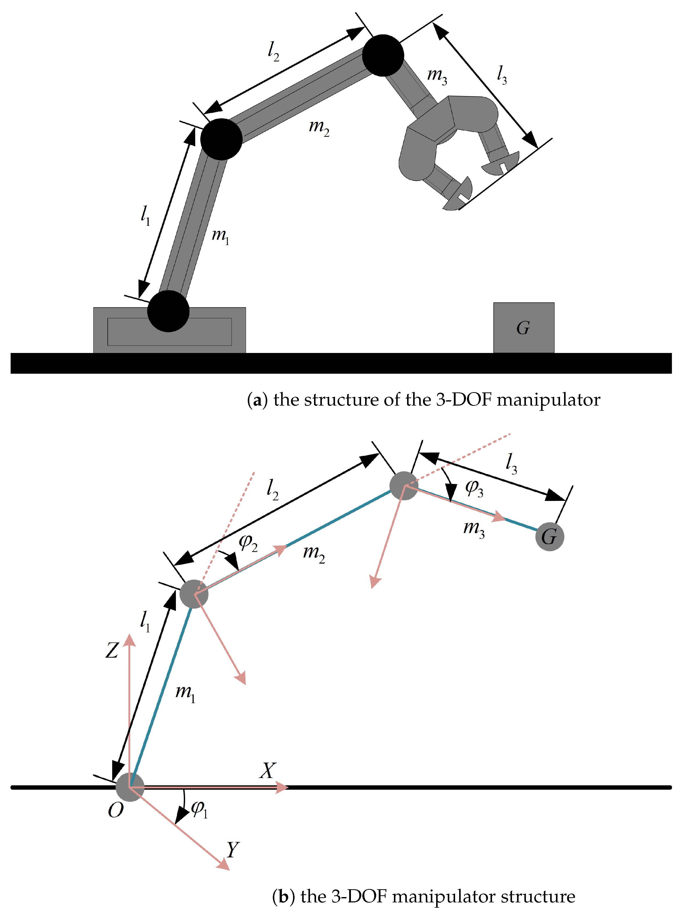
Figure 1. 3-DOF manipulator diagrams: (a) structural overview; (b) detailed configuration.
Processes 13 03638 g001
Figure 2. The timing diagram of the robust model predictive control.
Processes 13 03638 g002
Figure 3. A block diagram of the APRMPC algorithm.
Processes 13 03638 g003
Figure 4. Tracking errors of each joint with different parameters. (a) Joint 1 tracking error; (b) Joint 2 tracking error; (c) Joint 3 tracking error.
Processes 13 03638 g004
Figure 5. Comparison of tracking performance of each joint without unknown disturbances. (a) Tracking performance of Joint 1; (b) tracking performance of Joint 2; (c) tracking performance of Joint 3.
Processes 13 03638 g005
Figure 6. Comparison of tracking errors of each joint without unknown disturbances. (a) Tracking error of Joint 1; (b) tracking error of Joint 2; (c) tracking error of Joint 3.
Processes 13 03638 g006
Figure 7. Comparison of control inputs of each joint without unknown disturbances. (a) Control input of Joint 1; (b) control input of Joint 2; (c) control input of Joint 3.
Processes 13 03638 g007
Figure 8. Comparison of tracking performance of each joint under unknown disturbances. (a) Tracking performance of Joint 1; (b) tracking performance of Joint 2; (c) tracking performance of Joint 3.
Processes 13 03638 g008
Figure 9. Comparison of tracking errors of each joint under unknown disturbances. (a) Tracking error of Joint 1; (b) tracking error of Joint 2; (c) tracking error of Joint 3.
Processes 13 03638 g009
Figure 10. Comparison of control inputs of each joint under unknown disturbances. (a) Control input of Joint 1; (b) control input of Joint 2; (c) control input of Joint 3.
Processes 13 03638 g010
Table 1. Simulation parameters of the manipulator system.
ParametersSymbolsValues/Units
Mass of Link 1 m 1 5 kg
Mass of Link 2 m 2 8 kg
Mass of Link 3 m 3 10 kg
Length of Link 1 l 1 1.5 m
Length of Link 2 l 2 1.75 m
Length of Link 3 l 3 1.0 m
Gravitational Accelerationg 9.8 N / kg
Table 2. Performance indicators under different adaptive update rates.
Joint λ = 0.5 (rad) λ = 0.1 (rad) λ = 0.01 (rad)
Joint 1 8.74 × 10 4 5.82 × 10 4 3.15 × 10 4
Joint 2 7.89 × 10 4 4.93 × 10 4 2.87 × 10 4
Joint 3 9.12 × 10 4 6.01 × 10 4 3.42 × 10 4
Table 3. Performance indicators comparison.
Control AlgorithmRMSEIAFV
APRMPC 5.62 × 10 7 6.08 × 10 3
MPC 3.04 × 10 4 2.58 × 10 6
PID 2.51 × 10 2 1.26 × 10 8
Disclaimer/Publisher’s Note: The statements, opinions and data contained in all publications are solely those of the individual author(s) and contributor(s) and not of MDPI and/or the editor(s). MDPI and/or the editor(s) disclaim responsibility for any injury to people or property resulting from any ideas, methods, instructions or products referred to in the content.