Article

Predicting Oil Productivity of High Water Cut Fractured Horizontal Wells in Tight Oil Reservoirs Based on KAN

1
Twelfth Oil Production Plant, Changing Oilfield Company, Xi’an 710020, China
2
College of Petroleum Engineering, Yangtze University, Wuhan 430100, China
3
College of Resources and Environment, Yangtze University, Wuhan 430100, China
*
Authors to whom correspondence should be addressed.
Processes 2025, 13(11), 3629; https://doi.org/10.3390/pr13113629
Submission received: 29 September 2025 / Revised: 17 October 2025 / Accepted: 31 October 2025 / Published: 10 November 2025
(This article belongs to the Section Energy Systems)

Abstract

The high water cut period represents a critical phase in the development of tight oil wells, and accurately forecasting productivity during this stage is essential for effective oilfield development planning. However, traditional reservoir engineering methods find it difficult to handle complex oil-water seepage behaviors and cannot accurately predict the productivity of tight sandstone oil wells in the high water cut period. Therefore, this paper proposes a method for predicting the productivity of tight oil reservoirs based on a hybrid deep learning algorithm, using the geological, engineering, and development parameters of 342 fractured horizontal wells in the Z211 block of Heshui Oilfield. The model was based on the KAN deep learning algorithm, and the WOA meta-heuristic optimization algorithm was used to optimize the KAN model parameters. Combined with multi-dimensional parameters such as oil well geology, engineering and development, an efficient and accurate productivity prediction model was established. Based on the interpretability of the model itself, the key features of the model and the factors affecting productivity are explained in combination with the SHAP (SHapley Additive exPlanations) value and the Pearson coefficient, revealing the changing relationship of productivity and the degree of influence of different parameters on productivity. The results indicate that the KAN-WOA model demonstrates strong performance in both prediction accuracy and robustness for productivity forecasting. For high water cut fractured horizontal wells in tight oil reservoirs, water content and permeability were identified as the primary influencing factors on initial productivity, whereas for low water cut wells, dynamic liquid level, number of fracturing stages, and sand volume were the key determinants. This approach offers a novel data-driven solution for the development and management of tight oil wells, serving as an effective decision-support tool in oilfield development.

1. Introduction

Amid increasing global energy demand, tight oil and gas have become crucial unconventional resources attracting extensive attention [1]. However, a major challenge in developing tight oil wells is the accurate prediction of productivity during the high water-cut period [2]. Due to geological factors such as the inherently low matrix permeability of tight reservoirs and uneven fracture distribution, as well as development-related issues like complex injection-production dynamics and engineering influences such as volume fracturing, traditional reservoir engineering methods often fall short in providing reliable productivity forecasts [3,4,5]. Furthermore, the onset of the high water cut phase adds further complexity to productivity prediction. As tight oil reservoirs enter their middle to late stages of development, there is an urgent demand for more accurate predictive approaches to guide adjustments in development strategies [6].
The rise of machine learning technology has provided a new means to solve this problem. Through data-driven methods, effective information can be extracted from complex multidimensional data to make more accurate productivity predictions [7,8,9]. Scholars have already begun applying machine learning to production forecasting and fracture parameter optimization [10,11]. For instance, Luo et al. built a neural network model using well depth, perforation thickness, porosity, water saturation, fracture stages, fracturing fluid volume, and proppant amount to determine the relationship between oil production in the first year and key features [12]. Similarly, Wang & Chen analyzed 3610 fractured horizontal wells in the Montney reservoir in Canada and used artificial neural networks, support vector machines and other machine learning algorithms for prediction and evaluation [13]. Chen et al. developed a support vector machine (SVM)-based model to predict the initial productivity of horizontal wells in tight oil reservoirs [14]. However, studies have shown that existing machine learning approaches still struggle to accurately forecast the productivity of fractured horizontal wells during the high water cut period in tight oil reservoirs [6,15].
Kolmogorov–Arnold networks (KAN) are a new type of neural network architecture [16]. They use learnable activation functions and are superior to current MLP neural network architectures in terms of accuracy and interpretability and have performed well in multiple prediction tasks. However, the performance of KAN is highly sensitive to the setting of hyperparameters. The selection of parameters such as the number of grids, the order of spline functions, and the intensity of penalties will significantly affect the generalization ability and prediction accuracy of the model [17]. Traditional manual parameter tuning methods are not only time-consuming and laborious, but it is also difficult to ensure that the global optimal parameter combination is found. In addition, commonly used optimization methods such as grid search and random search are inefficient, especially when the dimension of the parameter space is high, the computational cost is expensive, and it is difficult to converge quickly [18]. In order to overcome these challenges, predecessors have proposed using meta-heuristic optimization algorithms to optimize the hyperparameters of the KAN model, such as PSO and WOA [19,20]. These intelligent global optimization algorithms can effectively explore the entire parameter space and avoid falling into local optimal solutions. They do not rely on gradient information, the parameter update process is simple, and are suitable for solving complex multi-dimensional optimization problems [21]. In oil well productivity forecasting, meta-heuristic optimization algorithms can automatically identify the optimal set of model parameters, enhancing the prediction accuracy of the KAN model while reducing the time required for parameter tuning.
The combination of machine learning (ML) and metaheuristic optimization algorithms has become a powerful tool for solving nonlinear and high-dimensional problems in petroleum engineering. Early foundational research demonstrated the potential of combining ensemble methods such as support vector machines (SVMs) and LightGBM with particle swarm optimization for production forecasting [22]. However, insufficient prediction accuracy persists. Furthermore, many deep learning models, while powerful, operate like “black boxes” and lack interpretability, a key obstacle to their application in high-risk oilfield development decision-making. In recent years, the emergence of explainable AI techniques, particularly SHAP (SHapley Additive ex-Planations), has begun to bridge this gap, enabling researchers to quantitatively attribute predictions to input features [23,24]. As an advanced model interpretability technology, SHAP’s core advantage is that it provides a unified, consistent, and theoretically sound explanation for any complex machine learning model.
This paper aims to use the KAN deep learning algorithm to construct a productivity prediction model for tight oil wells in the high water cut period based on multi-dimensional features such as oil well geology, engineering parameters and water content. Meanwhile, the WOA meta-heuristic optimization algorithm is employed to accelerate model convergence and achieve improved prediction performance. To further interpret the model’s output and enhance its explainability, the SHAP value method is applied to quantitatively assess the contribution of individual features. This enables an in-depth analysis of how geological and engineering parameters influence the productivity of horizontal wells in tight oil reservoirs, thereby offering a scientific basis for model-informed decision-making by oilfield engineers and supporting the optimization of development strategies.

2. Geology Background and Data Characteristics

The Ordos Basin, China’s second-largest sedimentary basin, consists of several structural units. The study area, the Z211 block of the Heshui Oilfield, is located within this basin (Figure 1). The reservoir is developed with gravity flow sedimentary sand dominated by sandy debris flows. The main production layer, C63, is a typical tight sandstone reservoir with an average effective thickness of 22.4 m, porosity of 10.4%, and permeability of 0.23 mD [25].
In 2012, the Z211 well area adopted a seven-point well network to carry out horizontal well water injection development tests. The water cut has been showing a steady upward trend since 2014. After the water injection into the oil wells took effect, it advanced rapidly along the high-permeability strips, with severe directional water breakthrough. It was difficult to expand the volume of the injected water, causing the water cut to rise faster after the oil wells broke through water. In addition, the reservoir had serious problems of multi-directional fracture-type water breakthrough and uneven unidirectional water drive. The directionality of water breakthrough was unclear, and the water cut remained high. The above reasons led to a large number of infill adjustment wells with high water cuts when they were put into production, which greatly restricted the productivity assessment and seriously affected the formulation of reservoir development plans.
In general, the key factors influencing volume fracturing in horizontal wells within tight oil reservoirs include geological parameters such as formation pressure, porosity, permeability, and oil saturation; engineering parameters like the number of fracturing stages, number of fracturing clusters, total sand volume, and total fluid volume; development parameters such as water cut and dynamic liquid level; as well as fluid properties including crude oil viscosity and density. The fluid properties in the study area are basically the same, so the geological, engineering, and development parameters in Figure 2 were mainly selected to carry out the productivity prediction study of fracturing horizontal wells.
In order to eliminate the impact of scale and make the machine learning model more convergent, we performed Z-Score standardization on the productivity dataset. This was conducted by subtracting the mean and dividing by the variance of each data point in the data, so that the processed data approximately conform to the standard normal distribution of (0, 1). The calculation formula is:
Z i * = Z i Z ¯ σ
Among them, Z i * is the standardized value, Z i is the original Z-factor, Z ¯ is the mean of the original data, σ is standard deviation of Z-factor. σ is calculated by the following formula:
σ = 1 n 1 i Z i Z ¯ 2
Following Z-Score standardization, the 324 productivity data samples were split into training and test sets at a ratio of 8:2. Within the training set, 20% of the data was designated as a validation set for model parameter optimization. The test set data were excluded from the training process and used solely to evaluate the model’s performance after training. Table 1 shows the data characteristics before and after Z-score processing.

3. Deep Learning Productivity Prediction Method

3.1. Principle of KAN Deep Learning Algorithm

Kolmogorov–Arnold Networks (KANs) represent an innovative deep learning framework derived from the Kolmogorov–Arnold representation theorem. This theorem asserts that any multivariate continuous function over a bounded domain can be represented as a finite combination of continuous univariate functions and binary addition operations. Different from the traditional MLP architecture deep learning algorithm, although KAN adopts a fully connected layer architecture as a whole, it puts the activation function on the edge to replace the weight parameters of the MLP architecture. Each activation function is represented by a one-dimensional function. In this way, the model only needs to sum the input features without any nonlinear operations. The number of parameters and training costs required for the overall model are greatly reduced compared to MLP.
The mathematical principle of KAN is the Kolmogorov–Arnold representation theorem, which is expressed as follows:
f x = f ( x 1 , , x n ) = q = 1 2 n + 1 Φ q p = 1 n ϕ q , p x p
where x 1 , , x n are input variables, ϕ q , p is a set of one-dimensional functions, Φ q is another set of functions defined in the real number domain. The theorem is expressed as an inner and outer summation. The inner layer is a weighted summation of each input variable x p , and the outer layer is the summation of 2n + 1 inner layers after being weighted by another set of functions.
KAN expands the basic mathematical theorem. In terms of model construction, it generalizes the network to any width and depth. The overall expression can be:
f x = i L 1 = 1 n L 1 ϕ L 1 , i L , i L 1 i L 2 = 1 n L 2 i 2 = 1 n 2 ϕ 2 , i 3 , i 2 i 1 = 1 n 1 ϕ 1 , i 2 , i 1 i 0 = 1 n 0 ϕ 0 , i 1 , i 0 x i 0
The specific description of the inner and outer layers is the same as that of the Kolmogorov–Arnold basic theorem.
Compared with complex and specific mathematical representations, we are more concerned with the concise abstract representation of KAN. The KAN model can be concisely represented as follows:
K A N x = Φ L 1 Φ L 2 Φ 1 Φ 0 x
Compared with the MLP architecture that places the weight W on the input edge, KAN places the activation function ϕ ( x ) on the edge for calculation. In the KAN neural network architecture, the output calculation of each layer is as follows (taking the lth layer as an example):
x l + 1 , j = i = 1 n l x ~ l , j , i = i = 1 n l ϕ l , j , i x l , i , j = 1 , , n l + 1
Its matrix expression is as follows:
x l + 1 = ϕ l , 1,1 ϕ l , 1 , n l ϕ l , 2,1 ϕ l , 2 , n l ) ϕ l , n l + 1 , 1 ϕ l , n l + 1 , n l Φ l x l
where Φl is the l th layer of KAN, n l + 1 is the number of nodes set for the l + 1 th layer, n l is the number of nodes set for the lth layer, and x l + 1 is the l + 1 th layer node after the l th layer node x l is activated and summed.
For the activation function ϕ ( x ) on each edge, KAN defines its representation as follows:
ϕ x = w b b x + w s s p l i n e x
The activation function is composed of the basis function b x and the spline function s p l i n e x . The weights w b and w s are used to adjust the size of the basis function and the spline function respectively to achieve better control of the overall amplitude of the activation function.
The basis function b x and the spline function s p l i n e x are defined as follows:
b ( x ) = x / ( 1 + e x )
s p l i n e x = i c i B i x
The basis function is a fixed one-dimensional function, and the spline function is represented by a linear combination of more subtle B i x spline functions [16]. Specifically, in a single grid, the spline function is composed of multiple B i x spline functions acting on different grid nodes. In the actual training process, KAN continuously changes the weight ci of the B i x spline function and refines the grid (as shown in Figure 3) to achieve the fitting effect and improve the prediction accuracy.
In this study, numerous key factors influence the productivity of horizontal wells in tight oil reservoirs, and the interrelationships among these factors are complex and intertwined. During the training process, KAN continuously adjusts the activation function, prunes relatively unimportant influencing factors and activation functions, and uses symbolic formulas for quantitative characterization, ultimately achieving prediction accuracy and interpretability.

3.2. WOA-KAN Productivity Forecast Model

The predictive performance of machine learning methods is heavily reliant on the quality and characteristics of the data, and different algorithms exhibit varying degrees of adaptability depending on specific data conditions. In addition, the setting of machine learning model parameters is very important for the results. In order to set appropriate KAN parameters, they can be optimized in a variety of ways, including manual debugging, using grid search or random search, etc. Table 2 lists some common KAN parameters, their meanings, and reference ranges.
Manual parameter tuning is often arbitrary, while grid search methods are time-consuming and labor-intensive. An alternative approach is to employ metaheuristic optimization algorithms for automatic parameter tuning. In this framework, the metaheuristic algorithm is embedded as an outer layer around the entire machine learning model, leveraging its automatic optimization capabilities to identify the optimal set of parameters. Metaheuristic algorithms such as genetic algorithms and particle swarm optimization are commonly used for this purpose [26]. In this study, the Whale Optimization Algorithm (WOA) was employed for model parameter tuning. WOA is a recently developed swarm intelligence algorithm and a form of metaheuristic optimization technique, inspired by the bubble-net feeding behavior of humpback whales. It is known for its simplicity, ease of implementation, low number of control parameters, and strong optimization performance. The fundamental principles and implementation process are outlined as follows:
  • Enclosure of prey
In the whale optimization algorithm, the search range encompasses the entire global solution space, and locating the prey is essential to encircle it. As the global optimum within the search space is unknown beforehand, the WOA algorithm assumes that the best candidate solution found so far represents the target prey or is approximately close to the global optimum [27]. Once the best search agent is identified, the remaining search agents update their positions in an attempt to move closer to this best agent. This behavior is governed by the following equation:
D = C X * t X t
X t + 1 = X * t A D
where t is the current iteration number, X * t is the position vector of the best whale, and X t is the position vector of the current whale. A and C are coefficient vectors. If there is a better solution, then X * t should be updated in each iteration. The calculation method of vectors A and C is as follows:
A = 2 a r a
C = 2 r
Here, the value of a decreases linearly from 2 to 0 over the course of iterations, while r is a random vector with elements uniformly distributed in the range [0, 1].
2.
Hunting behavior
Humpback whales employ two primary predation mechanisms: encirclement predation and bubble-net predation. The shrinking encirclement behavior is realized by gradually decreasing the value of a . In the bubble-net predation mode, the position update between the whale and the prey is modeled through a spiral equation that simulates the whale’s movement around the prey:
X t + 1 = D e b l cos 2 π l + X * t
D = X * t X t
Here, D represents the distance between the current search agent and the best-known solution; b is a constant that defines the spiral shape; and l is a random number uniformly distributed within the interval [−1, 1].
Since the algorithm includes two distinct strategies for approaching prey (bubble-net predation and shrinking encirclement), WOA selects one of them based on a probability value p. The corresponding position update formula is given as follows:
X t + 1 = X * t A D , 0 p 0.5 D e b l cos 2 π l + X * t , 0.5 p < 1
Here, p denotes the probability of selecting a specific predation mechanism, and it is randomly generated within the range [0, 1]. As the number of iterations t increases, both the parameter A and the convergence factor a decrease progressively. When A < 1 , the whales begin to converge around the current best solution, indicating that the algorithm has entered the local exploitation phase of the WOA.
3.
Searching for prey
To ensure that all whales are able to thoroughly explore the solution space, WOA updates their positions based on the distances between individuals, thereby facilitating random exploration. As a result, when A 1 , the search agent moves toward a randomly selected whale. The corresponding mathematical model is as follows:
D = C X r a n d t X t
X t + 1 = X r a n d t A D
Here, D represents the distance between the current search agent and a randomly selected individual, while X r a n d t denotes the position of that randomly selected individual at iteration t.
The WOA algorithm is used to optimize the parameters of the KAN model, and cross-validation is used in each iteration to improve the generalization ability of the model. After obtaining the optimal hyperparameter configuration, the training set is used to train and fit the prediction model to build the WOA-KAN productivity prediction model. Finally, the test set data are input, and the model performance is evaluated based on the prediction results obtained by the model. The prediction model process is shown in Figure 4.

3.3. Model Evaluation

The productivity evaluation model uses RMSE and the modified correlation coefficient R2 to evaluate the quality of the model. The smaller the RMSE, the more accurate the model prediction deviation factor. The larger the R2, the better the model performance. The calculation formula is as follows [28]:
R M S E = 1 N i = 1 N Z i Z p r e d 2
r 2 = 1 i = 1 N Z i Z p r e d 2 i = 1 N Z i Z ¯ 2
R 2 = 1 1 r 2 N 1 N m 1

4. Productivity Forecast Results

4.1. Comparison of Prediction Performance of Different Models

This study set the maximum number of iterations to 50, and when the validation error no longer decreased significantly (i.e., the global optimal solution does not improve significantly in multiple consecutive iterations), the optimization process was terminated early. The preset hyperparameters in the model are shown in Table 3. Finally, WOA converged to the optimal parameter combination. The mean square error of the KAN model optimized by WOA on the test set was 0.035, which was 39.7% less than the unoptimized default parameter model (MSE = 0.058). Compared with the traditional grid search parameter adjustment (MSE = 0.042), WOA optimization also achieved lower error and significantly improved computational efficiency. Figure 5a shows the convergence curve of the validation error during the WOA optimization process. It can be seen that WOA quickly reduced the validation error after about 38 iterations, and then the error gradually converged. After 38 iterations, the error tended to stabilize, indicating that the model had reached the global optimal solution. Figure 5b displays the variation in the loss function on both the training and test datasets before and after optimization using the WOA algorithm. The blue curve represents the training set loss, while the orange curve corresponds to the test set loss. It is evident that prior to optimization, the loss function required approximately 15 iterations to stabilize. In contrast, after applying WOA optimization, the loss decreased significantly and stabilized within 10 iterations. This indicates that the model achieved faster and more stable convergence following WOA optimization. In terms of overall loss, the test loss of the model before optimization was about 0.6, and the test loss after optimization was about 0.06. The overall loss before and after optimization was significantly reduced by one order of magnitude, which reflects the power of the WOA algorithm in parameter optimization. In general, WOA optimization significantly improved the performance of KAN model in oil well productivity prediction. Through the global search mechanism, a better parameter combination was found. Compared with the traditional parameter adjustment method, WOA not only has a significant reduction in error, but also improves the efficiency of parameter adjustment. The experimental results show that WOA exhibits a strong global optimization ability in high-dimensional parameter space, can effectively avoid the problem of local optimal solution, and is particularly suitable for complex nonlinear prediction tasks.
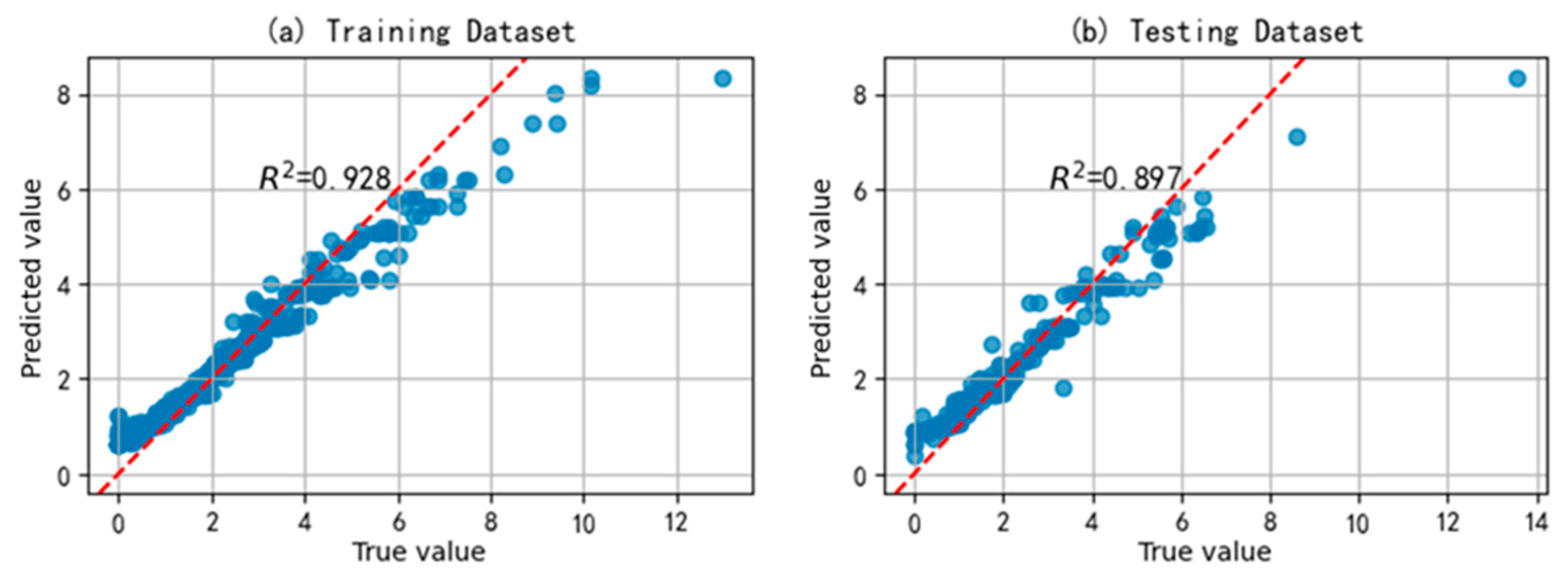
Figure 6 demonstrates the prediction performance of the KAN-WOA model on both the training and test datasets. The predicted productivity values from the KAN model showed a strong agreement with the actual measured values. In the scatter plot, blue points represent the comparison between predicted and actual values, while the red dashed line denotes the ideal 45° reference line, indicating perfect prediction accuracy. On the training set, the model achieved a coefficient of determination (R2) of 0.928, reflecting excellent fitting capability. On the test set, the R2 value reached 0.897, indicating that the model maintained strong generalization ability, with predicted values remaining highly correlated with actual productivity. These results confirm that the proposed model in this study can effectively and accurately predict the initial productivity of fractured horizontal wells in tight oil reservoirs.
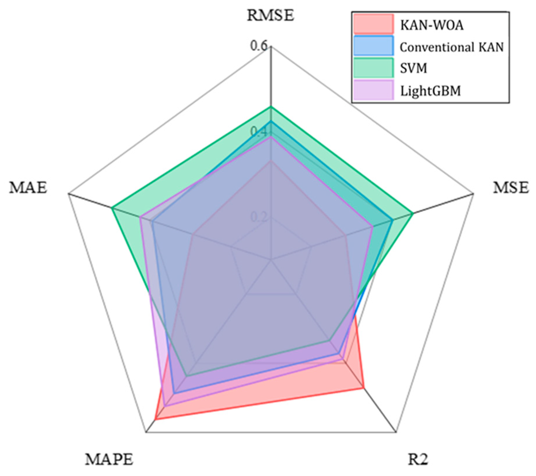
In order to reflect the advanced nature of the model proposed in this paper, it was compared with the conventional KAN, SVM, and LightGBM models. Figure 7 shows the comprehensive performance comparison of the four models of KAN-WOA, conventional KAN, SVM, and LightGBM under multiple evaluation indicators. The different colors in the radar chart represent the performance of each model, among which KAN-WOA performed well in multiple dimensions and had the largest coverage area, indicating that it was superior to other models in these indicators. The performance of conventional KAN and SVM was similar, with small differences in most dimensions, but conventional KAN had a slight advantage in some indicators. In contrast, LightGBM was slightly inferior to other models in overall performance, especially in some dimensions, where it was significantly weaker than KAN-WOA. Overall, the KAN-WOA model proposed in this paper showed the best performance in various evaluation indicators. Table 4 illustrates the specific values for different models under various evaluation indicators.

4.2. Explanatory Analysis of Factors Affecting KAN Productivity Combined with SHAP Value

Compared with other machine learning models, the advantages of the KAN model are not only reflected in its prediction accuracy, but also in its strong interpretability. Most machine learning algorithms, such as XGBoost and MLP, are usually regarded as “black boxes” due to the complexity of their internal models, and their interpretability is limited. In the construction of the KAN model, the expression of the activation function is clearly defined, and in the subsequent training, the form of the activation function is continuously adjusted by controlling the number of segments and order of the spline function, so that the activation function expression corresponding to each neuron in the model is specific and fixed. On this basis, KAN introduces model construction diagrams and symbolic representations to achieve intuitive analysis of the interpretability of influencing factors.
On the other hand, SHAP is increasingly being applied in the interpretation of machine learning models to illustrate the contribution of each feature in a single sample to the model’s prediction outcome [29]. Rooted in the Shapley value concept from game theory, SHAP effectively interprets both the prediction mechanism and feature importance within machine learning models [30]. The SHAP value represents the extent to which an individual input feature contributes to the model’s output, helping to uncover thresholds and interaction effects between explanatory variables and the target variable. The formula for calculating the SHAP value is as follows:
S H A P f , x , S = T S T ! n T ! n ! f x f x S / T
Here, f represents the prediction function of the model; x denotes the observed feature vector; S is the set of all input features; n is the total number of features; and x S / T refers to the observed values of all features excluding the feature T.
Therefore, this paper conducted an interpretability analysis of key influencing factors based on the interpretability of KAN itself and combined with the SHAP value. First, the key influencing factors and output results were simply quantitatively characterized using KAN’s own model diagram and symbolic formula. Then, the SHAP value was utilized to represent both the direction (positive or negative) and the magnitude of each feature’s influence on the model’s prediction outcome, further improving the interpretability analysis effect. Finally, a heat map was used to analyze the correlation between different parameters and oil well productivity.
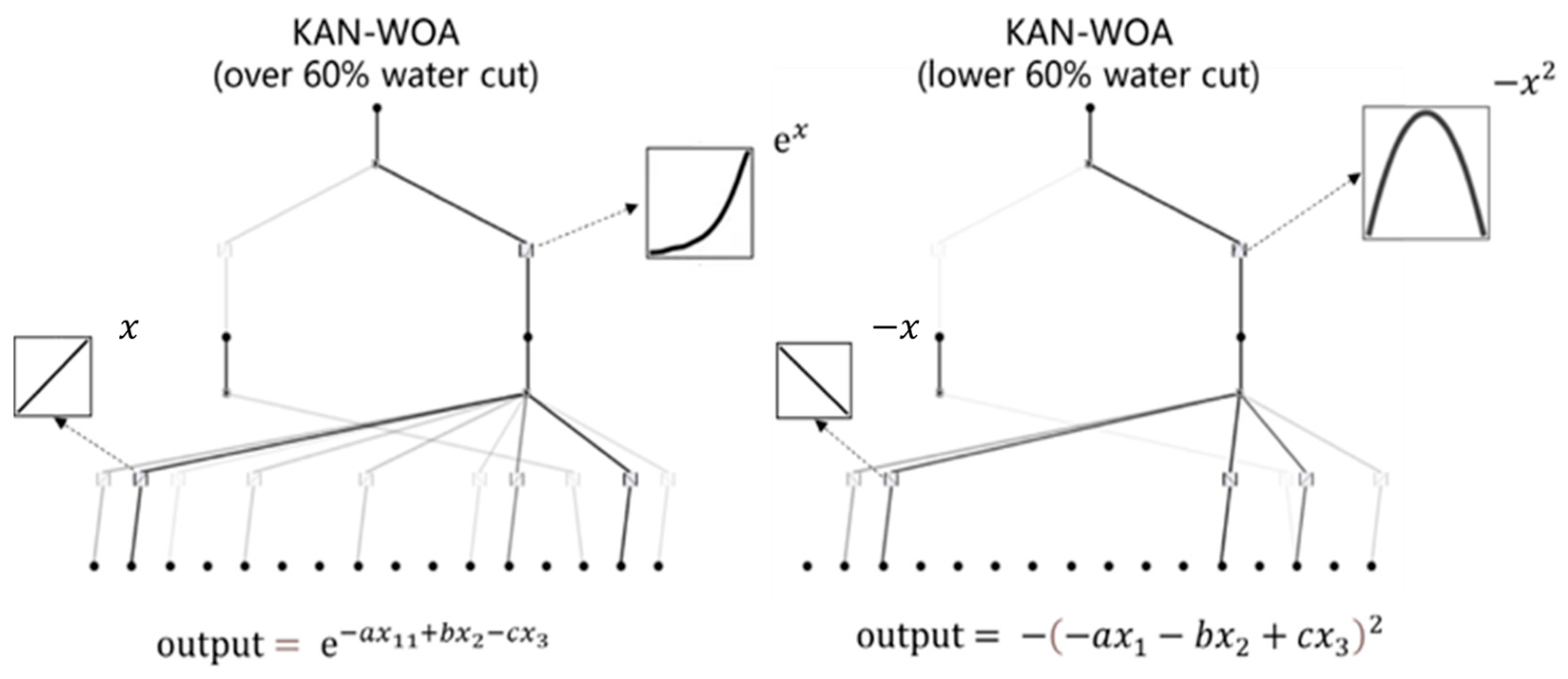
First, we generated the model structure diagram of the KAN-WOA model when the moisture content was higher than 60% and lower than 60% (as shown in Figure 8).
In the model structure diagram, the depth of the black solid line represents the influence of the input features. The darker the color, the greater the influence. In this model construction, we adopted a classic three-layer architecture, consisting of an input layer as the first layer, a nonlinear hidden layer as the second (intermediate) layer, and an output layer as the third layer. By generating a structure diagram of the model under different water contents, we can see that in the water content stage with a water content higher than 60%, there were two main factors that affected the model output, and there were more secondary factors. The main factors and secondary factors were linearly combined, and the prediction results were output after nonlinear processing of the hidden layer; in the water content stage with a water content lower than 60%, there were three main factors that affected the model output, and there were relatively few secondary factors. The main factors and secondary factors were also linearly combined, and the prediction results were output after nonlinear processing of the hidden layer.
To further analyze the relationship between input features and output results, we used KAN’s symbolic formula for quantitative representation. Since there were more than a dozen input features in this model, we only took the first three most important features for symbolic representation. The symbolic formula representation results are shown in Figure 9.
It can be seen that in the water-containing stage with a moisture content higher than 60%, the output result was in the form of an exponential function, indicating that the yield changes greatly with the main influencing characteristics. In the water-containing stage with a moisture content lower than 60%, the output result was in the form of a quadratic function, indicating that the yield also changes greatly with the main influencing characteristics and reaches a peak during the change process.
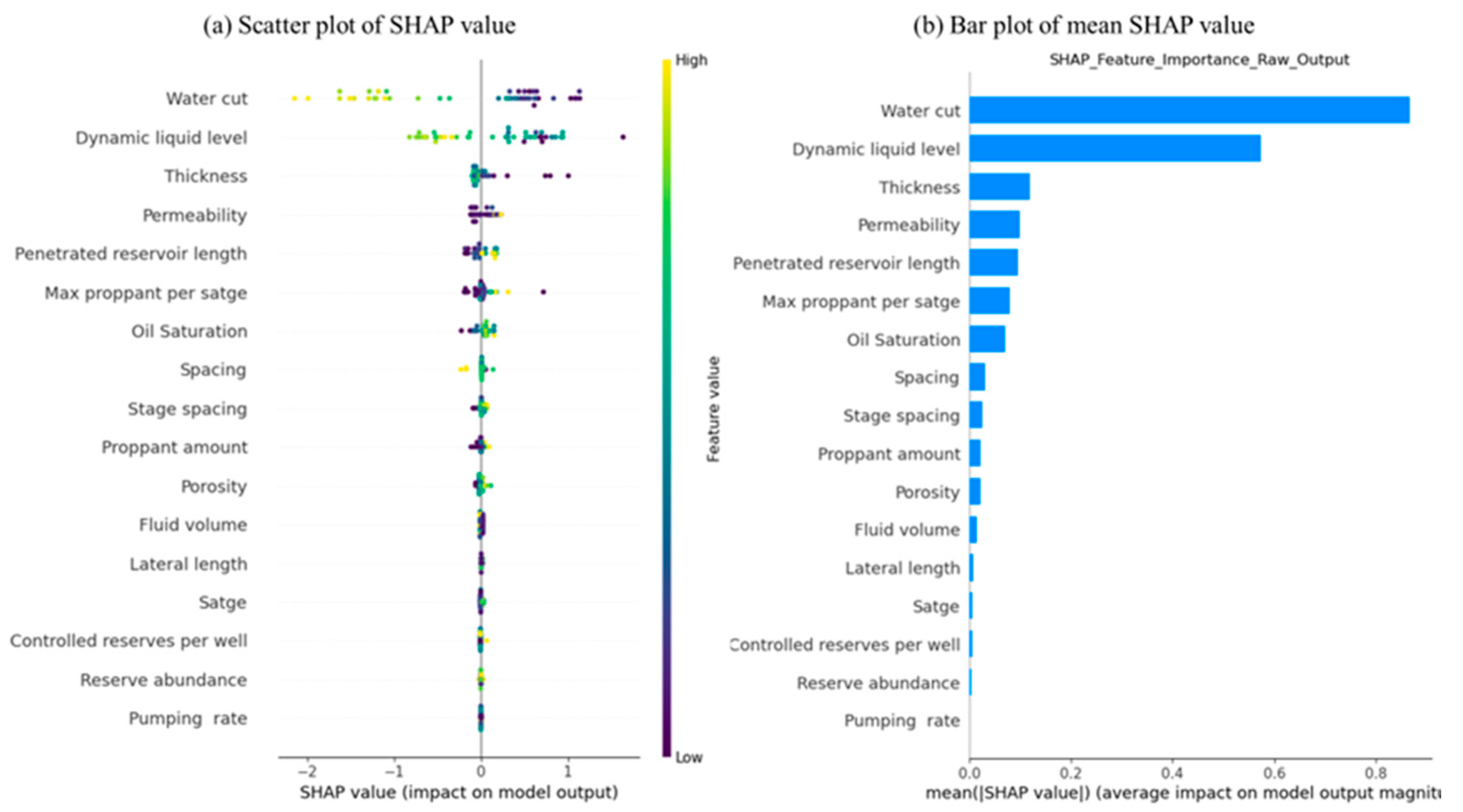
In terms of the interpretability of the KAN model itself, this paper introduced the SHAP value to identify key influencing features and their degree of influence. Through SHAP value analysis, this paper identified several key features that contributed most to productivity prediction. In Figure 10a, each point represents a specific feature value of a sample and its contribution to the model prediction. The horizontal axis is the SHAP value, which indicates the intensity and direction of the feature’s influence on the model output. When the SHAP value is positive, the feature will drive the model prediction value higher; when it is negative, the feature will cause the prediction value to decrease. The color of the point ranges from yellow (high feature value) to blue (low feature value) to indicate different feature value ranges. The SHAP value shows that the water cut and the dynamic surface of the high water cut fractured horizontal well had a strong negative correlation with the productivity. Figure 10b presents the average influence of each feature on the model output, expressed as the absolute mean of the SHAP values. This metric was used to evaluate the relative importance of each feature within the model. The results indicate that water cut was the most influential feature affecting the model’s predictions. Geological features such as permeability and vertical thickness of the reservoir had a greater impact on the productivity of high water cut fractured horizontal wells. The SHAP value results align with practical understanding, indicating that the pronounced heterogeneity and reservoir characteristics of tight sandstone formations are the primary factors contributing to the high water content observed in oil wells.
For oil wells with a water content below 60%, the primary factors influencing productivity were the dynamic liquid level, the number of fracturing stages, and the amount of sand injected (Figure 11). Among these, the dynamic liquid level typically exhibited a significant negative correlation with productivity. Variations in dynamic liquid level can provide insights into reservoir pressure, wellbore production conditions, formation flow capacity, and the operational status of downhole equipment. The rise of the dynamic liquid level usually indicates that the reservoir pressure is decreasing, the natural driving force of the fluid is weakened, and the productivity of the oil well may be decreasing. Engineering parameters such as the number of reforming stages, the amount of liquid entering the ground and the amount of sand added have a positive impact on the productivity. The larger the scale of the tight oil reservoir reforming, the higher the productivity of the oil well is generally. Therefore, based on the SHAP value analysis presented in Figure 10 and Figure 11, it can be concluded that water content and geological factors exert the most significant influence on the productivity of fractured horizontal wells during the high water cut stage in tight oil reservoirs. In contrast, engineering factors play a more prominent role in affecting productivity during the low water cut stage.
For high water cut wells (>60%), tight sandstones are characterized by extreme microscopic pore-throat heterogeneity and complex macroscopic permeability contrasts. After prolonged production, injected water or aquifer water preferentially travels through the high-permeability “streaks” or fractures, bypassing a significant volume of oil trapped in lower-permeability zones. This phenomenon, known as “heterogeneous tongue-in” or “fingering”, is the primary reason for the dominance of permeability. The model learns that the permeability distribution, which governs these flow paths, is the ultimate controller of water breakthrough timing and subsequent water cut rise [31]. In addition, once a well is in a high water-cut state, the relative permeability to water dominates the flow system. The current water cut is a direct measure of the fractional flow of water in the wellbore and reflects the maturity of these water channels. A higher initial water cut for prediction suggests that these preferential channels are already well-established, making the future production trend heavily dependent on the stability and expansion of these water-dominated flow paths. In a highly heterogeneous tight sandstone, this effect is amplified. The contrast between high-perm and low-perm zones is more severe, leading to rapid water breakthrough and a quicker rise to high water [32].
For low water cut wells (≤60%), the flow behavior was dominated by the effectiveness of the stimulated reservoir volume (SRV) created by hydraulic fracturing, rather than by the natural permeability heterogeneity at this early production stage. In low-permeability tight sandstones, a sufficient and stable drawdown is critical to overcome the significant capillary forces and flow resistance in the nano-Darcy scale matrix. A deeper fluid level (higher drawdown) helps to mobilize hydrocarbons from the tight matrix into the more conductive fracture network. Its dominance in the model underscores that energy availability and effective pressure differential are the primary drivers of initial production, before water breakthrough occurs. The number of fracturing stages and sand volume are key design parameters that directly determine the geometry and conductivity of the artificial fracture network. Fracturing stages control the lateral coverage and complexity of the SRV, ensuring that a larger volume of the reservoir is connected to the wellbore. Proppant volume primarily determines the conductivity and long-term stability of the created fractures. Sufficient proppant prevents fracture closure under in situ stress, maintaining high-flow pathways.
To further examine the relationship between various parameters and oil well productivity, the Pearson correlation coefficient was employed to quantify the linear association between each parameter and productivity. The correlation coefficient varies between −1 and 1, where a value of 1 represents a perfect positive linear correlation, −1 indicates a perfect negative linear correlation, and 0 signifies no linear correlation between the variables. By calculating the correlation matrix, we can quantify the strength of the relationship between each factor and oil well productivity. A heat map was drawn based on the correlation matrix. The color coding of the heat map reflects the size and direction of the correlation coefficient. Dark red represents a strong positive correlation, dark blue signifies a strong negative correlation, while colors close to white indicate weak or negligible correlation. The corresponding correlation coefficient value is marked in each cell of the heat map, which facilitates accurate comparison of the relationship between various factors [33].
Figure 12 shows the heat map of the correlation between the productivity of low water cut oil wells and high water cut oil wells. The results indicate that when the water cut was below 60%, the number of fracturing stages exhibited a significant positive correlation with oil well productivity, with a correlation coefficient of 0.56. This suggests that an increase in the number of fracturing stages corresponds to higher oil well productivity. Similarly, the amount of sand added (correlation coefficient = 0.78) and the amount of liquid used (correlation coefficient = 0.69) were also strongly positively correlated with the productivity, while the dynamic liquid level was strongly negatively correlated with the productivity, which is consistent with the expected impact of the SHAP value on productivity. When the water cut was greater than 60, the water cut (correlation coefficient = −0.72) was strongly negatively correlated with the productivity of the oil well, which means that an increase in water cut will significantly reduce the productivity of the oil well. In addition, the well spacing also showed a negative correlation, further verifying the trend that the productivity of the oil well is negatively affected by the development parameters. The results shown in the heat map further verify the explanation of the model by the SHAP value and the reliability of the model proposed in this paper.

5. Conclusions

The main contributions of this paper are as follows:
(1)
The WOA algorithm was integrated with the KAN model and applied to the domain of oil well productivity prediction. By leveraging the global search capability of WOA, the selection of model hyperparameters was substantially optimized. Experimental results demonstrate that this approach not only enhances prediction accuracy but also improves computational efficiency. Compared with traditional parameter adjustment methods, WOA showed better stability and robustness when processing complex datasets, providing an efficient path for the construction of oil well productivity prediction models.
(2)
Based on the interpretability of the model itself, combined with the SHAP value and correlation heat map, the trend of productivity changes with influencing factors and the correlation between influencing factors and productivity were systematically analyzed.
In summary, this paper constructed the WOA-KAN model by modeling and regression analysis of geological, engineering, and production data of oil wells, showing high prediction accuracy and stability. The analysis method combined with the SHAP value revealed the significant impact of water content, permeability, and other characteristics on the productivity of high water cut oil wells, providing an important reference for scientific decision-making in oilfield development.

Author Contributions

Conceptualization, H.Z. (Hongjun Zhang) and T.Y.; methodology, D.Z.; validation, H.Z. (Hongbo Zhang); formal analysis, Y.Z.; investigation, R.X.; resources, D.Z.; data curation, H.Z. (Hongjun Zhang); writing—original draft preparation, T.Y.; writing—review and editing, Z.Z.; visualization, Z.W. All authors have read and agreed to the published version of the manuscript.

Funding

This research was funded by the Xinjiang Uygur Autonomous Region Natural Science Foundation Youth Science, grant number 2025D01B153.

Data Availability Statement

The data are available from the corresponding author on reasonable request.

Conflicts of Interest

Authors Hongjun Zhang, Tao Yi, Dalin Zhou, Hongbo Zhang, Yuyang Zhang and Rui Xue were employed by Changing Oilfield Company. The remaining authors declare that the research was conducted in the absence of any commercial or financial relationships that could be construed as a potential conflict of interest.

References

  1. Geng, S.; Li, C.; Li, Y.; Zhai, S.; Xu, T.; Gong, Y.; Jing, M. Pressure transient analysis for multi-stage fractured horizontal wells considering threshold pressure gradient and stress sensitivity in tight sandstone gas reservoirs. Gas Sci. Eng. 2023, 116, 205030. [Google Scholar] [CrossRef]
  2. Liu, Z.-B.; Liu, H.-H. An effective method to predict oil recovery in high water cut stage. J. Hydrodyn. 2015, 27, 988–995. [Google Scholar] [CrossRef]
  3. Shen, A.; Liu, Y.; Wang, X.; Cai, B.; He, C.; Liang, S. The geological characteristics and exploration of continental tight oil: An investigation in China. J. Pet. Explor. Prod. Technol. 2019, 9, 1651–1658. [Google Scholar] [CrossRef]
  4. Wang, J.; Liu, S.; Li, J.; Zhang, Y.; Gao, L. Characteristics and causes of Mesozoic reservoirs with extra-low permeability and high water cut in northern Shaanxi. Pet. Explor. Dev. 2011, 38, 583–588. [Google Scholar] [CrossRef]
  5. Yang, H. Characteristics and resource prospects of tight oil and shale oil in Ordos Basin. Acta Pet. Sin. 2013, 34, 1–11. [Google Scholar]
  6. Wang, H.; Mu, L.; Shi, F.; Dou, H. Production prediction at ultra-high water cut stage via Recurrent Neural Network. Pet. Explor. Dev. 2020, 47, 1084–1090. [Google Scholar] [CrossRef]
  7. Aydin, G. Regression models for forecasting global oil production. Pet. Sci. Technol. 2015, 33, 1822–1828. [Google Scholar] [CrossRef]
  8. Sen, D.; Hamurcuoglu, K.I.; Ersoy, M.Z.; Tunç, K.M.M.; Günay, M.E. Forecasting long-term world annual natural gas production by machine learning. Resour. Policy 2023, 80, 103224. [Google Scholar] [CrossRef]
  9. Zhai, S.; Geng, S.; Li, C.; Gong, Y.; Jing, M.; Li, Y. Prediction of gas production potential based on machine learning in shale gas field: A case study. Energy Sources Part A Recovery Util. Environ. Eff. 2022, 44, 6581–6601. [Google Scholar] [CrossRef]
  10. Davtyan, A.; Rodin, A.; Muchnik, I.; Romashkin, A. Oil production forecast models based on sliding window regression. J. Pet. Sci. Eng. 2020, 195, 107916. [Google Scholar] [CrossRef]
  11. Ibrahim, N.M.; Alharbi, A.A.; Alzahrani, T.A.; Abdulkarim, A.M.; Alessa, I.A.; Hameed, A.M.; Albabtain, A.S.; Alqahtani, D.A.; Alsawwaf, M.K.; Almuqhim, A.A. Well performance classification and prediction: Deep learning and machine learning long term regression experiments on oil, gas, and water production. Sensors 2022, 22, 5326. [Google Scholar] [CrossRef] [PubMed]
  12. Luo, G.; Tian, Y.; Bychina, M.; Ehlig-Economides, C. Production Optimization Using Machine Learning in Bakken Shale. In Proceedings of the SPE/AAPG/SEG Unconventional Resources Technology Conference, Houston, TX, USA, 23–25 July 2018. [Google Scholar]
  13. Wang, S.; Chen, S. Insights to fracture stimulation design in unconventional reservoirs based on machine learning modeling. J. Pet. Sci. Eng. 2019, 174, 682–695. [Google Scholar] [CrossRef]
  14. Chen, H.; Zhang, C.; Xu, C.; Wang, Z.; Li, F.; Shang, Y.; Zhang, S.; Li, X. Support vector machine-based initial productivity prediction for SRV of horizontal wells in tight oil reservoirs. China Offshore Oil Gas 2022, 34, 102–109. [Google Scholar]
  15. Suhag, A.; Ranjith, R.; Aminzadeh, F. Comparison of shale oil production forecasting using empirical methods and artificial neural networks. In Proceedings of the SPE Annual Technical Conference and Exhibition, San Antonio, TX, USA, 9–11 October 2017. [Google Scholar]
  16. Liu, Z.; Wang, Y.; Vaidya, S.; Ruehle, F.; Halverson, J.; Soljačić, M.; Hou, T.Y.; Tegmark, M. Kan: Kolmogorov-arnold networks. arXiv 2024, arXiv:2404.19756. [Google Scholar] [PubMed]
  17. Hu, Y.; Xin, X.; Yu, G.; Deng, W. Deep insight: An efficient hybrid model for oil well production forecasting using spatio-temporal convolutional networks and Kolmogorov–Arnold networks. Sci. Rep. 2025, 15, 8221. [Google Scholar] [CrossRef]
  18. Geng, S.; Zhai, S.; Li, C. Swin transformer based transfer learning model for predicting porous media permeability from 2D images. Comput. Geotech. 2024, 168, 106177. [Google Scholar] [CrossRef]
  19. Qiu, Y.; Zhou, J.; Khandelwal, M.; Yang, H.; Yang, P.; Li, C. Performance evaluation of hybrid WOA-XGBoost, GWO-XGBoost and BO-XGBoost models to predict blast-induced ground vibration. Eng. Comput. 2022, 38 (Suppl. S5), 4145–4162. [Google Scholar] [CrossRef]
  20. Zivkovic, M.; Bacanin, N.; Antonijevic, M.; Nikolic, B.; Kvascev, G.; Marjanovic, M.; Savanovic, N. Hybrid CNN and XGBoost model tuned by modified arithmetic optimization algorithm for COVID-19 early diagnostics from X-ray images. Electronics 2022, 11, 3798. [Google Scholar] [CrossRef]
  21. Ekanayake, I.; Palitha, S.; Gamage, S.; Meddage, D.; Wijesooriya, K.; Mohotti, D. Predicting adhesion strength of micropatterned surfaces using gradient boosting models and explainable artificial intelligence visualizations. Mater. Today Commun. 2023, 36, 106545. [Google Scholar] [CrossRef]
  22. Liu, X.; Zhang, T.; Yang, H.; Qian, S.; Dong, Z.; Li, W.; Zou, L.; Liu, Z.; Wang, Z.; Zhang, T.; et al. Explainable Machine Learning-Based Method for Fracturing Prediction of Horizontal Shale Oil Wells. Processes 2023, 11, 2520. [Google Scholar] [CrossRef]
  23. Ma, X.; Hou, M.; Zhan, J.; Liu, Z. Interpretable Predictive Modeling of Tight Gas Well Productivity with SHAP and LIME Techniques. Energies 2023, 16, 3653. [Google Scholar] [CrossRef]
  24. Kim, H.-S.; Kim, H.-S.; Choi, S.-Y. Investigating the Impact of Agricultural, Financial, Economic, and Political Factors on Oil Forward Prices and Volatility: A SHAP Analysis. Energies 2024, 17, 1001. [Google Scholar] [CrossRef]
  25. Ma, Y.-Q.; Zhang, C.; Lu, Y.-C.; Kong, X.-Y.; Guo, Y.; Dong, Y.-X.; Chen, L.; Qi, R.; Xing, F.-C. Characteristics, main controlling factors and densification mechanisms of unconventional tight reservoirs in Triassic Yanchang Formation in southern Ordos Basin, China. Pet. Sci. 2024, 21, 3884–3898. [Google Scholar] [CrossRef]
  26. Mirjalili, S.; Lewis, A. The whale optimization algorithm. Adv. Eng. Softw. 2016, 95, 51–67. [Google Scholar] [CrossRef]
  27. Cao, W.; Zhou, J.; Xu, Q.; Zhen, J.; Huang, X. Short-Term Forecasting and Uncertainty Analysis of Photovoltaic Power Based on the FCM-WOA-BILSTM Model. Front. Energy Res. 2022, 10, 926774. [Google Scholar] [CrossRef]
  28. Geng, S.; Zhai, S.; Ye, J.; Gao, Y.; Luo, H.; Li, C.; Liu, X.; Liu, S. Decoupling and predicting natural gas deviation factor using machine learning methods. Sci. Rep. 2024, 14, 21640. [Google Scholar] [CrossRef] [PubMed]
  29. Ekanayake, I.; Meddage, D.; Rathnayake, U. A novel approach to explain the black-box nature of machine learning in compressive strength predictions of concrete using Shapley additive explanations (SHAP). Case Stud. Constr. Mater. 2022, 16, e01059. [Google Scholar] [CrossRef]
  30. Mangalathu, S.; Hwang, S.-H.; Jeon, J.-S. Failure mode and effects analysis of RC members based on machine-learning-based SHapley Additive exPlanations (SHAP) approach. Eng. Struct. 2020, 219, 110927. [Google Scholar] [CrossRef]
  31. Jin, Y.; Guo, K.; Gao, X.; Li, Q. Tight Oil Well Productivity Prediction Model Based on Neural Network. Processes 2024, 12, 2088. [Google Scholar] [CrossRef]
  32. Zhao, K.; Du, P. A new production prediction model for multistage fractured horizontal well in tight oil reservoirs. Adv. Geo-Energy Res. 2020, 4, 152–161. [Google Scholar] [CrossRef]
  33. Gu, Z.; Eils, R.; Schlesner, M. Complex heatmaps reveal patterns and correlations in multidimensional genomic data. Bioinformatics 2016, 32, 2847–2849. [Google Scholar] [CrossRef] [PubMed]
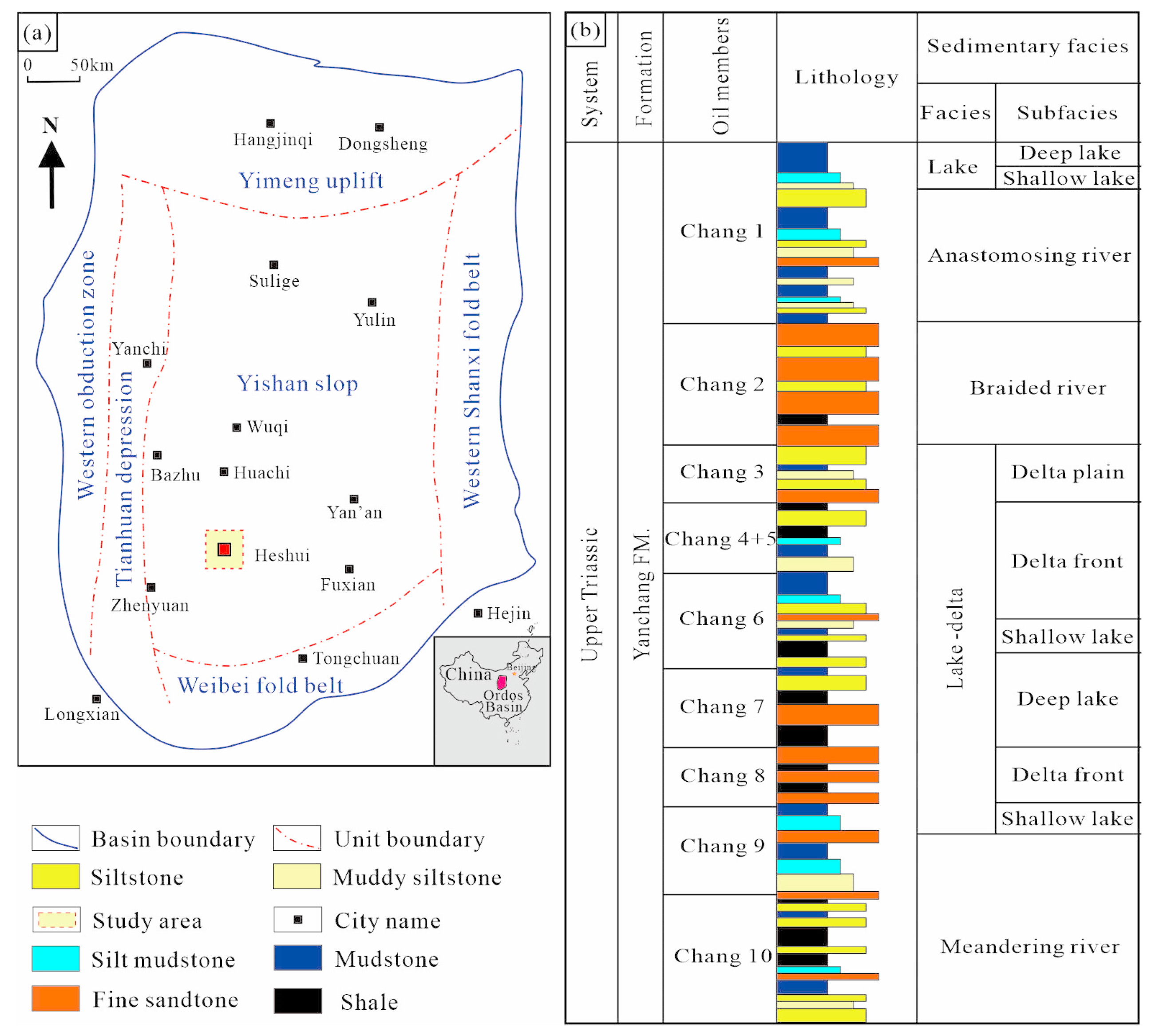
Figure 1. (a) Geographical location map of the research work area; (b) Study of the stratigraphic sequence columnar section of the target stratigraphic layer in the research area.
Processes 13 03629 g001
Figure 2. Box plot of oil productivity and influencing factors.
Processes 13 03629 g002
Figure 3. KAN architecture and training process diagram.
Processes 13 03629 g003
Figure 4. WOA-KAN Productivity Forecast Model. The red arrow indicates that WOA passes the hyperparameters of the trained KAN model to the KAN model.
Processes 13 03629 g004
Figure 5. (a) Fitness function curve of WOA optimization process; (b) Comparison of loss function reduction before and after WOA optimization.
Processes 13 03629 g005
Figure 6. (a) Scatter plot of model predictions versus actual productivity on the training set; (b) Scatter plot of model predictions versus actual productivity on the test set.
Processes 13 03629 g006
Figure 7. Radar chart comparing the performance of different productivity prediction models.
Processes 13 03629 g007
Figure 8. Model structure when the water cut is greater than 60% and less than 60%.
Processes 13 03629 g008
Figure 9. Model input–output relationship diagram under the introduction of symbolic formula.
Processes 13 03629 g009
Figure 10. (a) SHAP value scatter plot for wells with water cut greater than 60%; (b) SHAP value bar chart for wells with water cut greater than 60%.
Processes 13 03629 g010
Figure 11. (a) SHAP value scatter plot for wells with water cut less than 60%; (b) SHAP value bar chart for wells with water cut less than 60%.
Processes 13 03629 g011
Figure 12. (a) Heat map of oil productivity influencing factors with water cut more than 60%; (b) Heat map of oil productivity influencing factors with water cut less than 60%.
Processes 13 03629 g012
Table 1. Characteristics of data before and after Z-score processing.
VariableValue Before Z-ScoreValue Before Z-Score
MaxMinMeanMedianStd.MaxMinMeanMedianStd.
Spacing750200469.2850073.103.84−3.6800.421
Lateral Length2091200863.20761357.823.43−1.85−0.29
Controlled Reserve Per Well49.942.6219.0418.038.413.67−1.95−0.12
Penetrated
Reservoir Length
1889.9036712.69641.27328.223.59−2.06−0.22
Permeability0.990.070.200.1750.108.13−1.33−0.25
Porosity16.906.6310.2010.21.076.28−3.350.00
Oil Saturation72.8941.2556.2056.394.753.51−3.150.04
Thickness21.200.712.8712.673.762.22−3.24−0.05
Fracturing Stages33411.60104.674.58−1.63−0.34
Stage Spacing2386064.9764.84529.845.80−2.180.00
Proppant Amount5544.50160924.69596.2855.945.40−0.89−0.38
Max Proppant
Per Stage
256.9018.383.0864.744.913.87−1.44−0.41
Pumping Rate24.4426.5962.866.23−1.60−0.21
Fluid Volume37,749.1015217768.405336.65906.155.08−1.06−0.41
Water Cut100034.6028.0523.422.79−1.48−0.28
Dynamic Liquid Level14361791104.161160209.101.59−4.420.27
Oil Productivity13.5702.672.231.925.67−1.39−0.23
Table 2. Physical meaning and reference range of KAN model parameters.
ParameterPhysical MeaningReference Range
width (width)The number of nodes per layer of the model1–10
grid
(number of grid nodes)
The number of B-splines per spline activation function5–10
K (degree)The order of the B-spline function3–5
steps
(number of training rounds)
Control the training rounds of the model to avoid underfitting or overfitting10–200
opt (optimizer type)Optimize each model training to improve convergence speedLBFGS, Adam
loss_fn (loss function)Measuring model prediction errorMSE, CrossEntropy
lambda
(L2 regularization term)
Control parameter size and improve model generalization ability0–0.1
lamb_entropy
(entropy regularization coefficient)
Control the complexity of the spline function to improve the accuracy of the model1–50
Table 3. KAN and WOA model parameter settings.
ModelParametersValue
NetworkMaximal depth4
Maximal number of neurons per hidden layer5
Maximal grid value64
WOAPopulation size30
Max iteration50
Dimensions of the problem3
Table 4. Specific numerical values of different model evaluation indicators.
KAN-WOAConventional KANSVMLightGBM
RMSE0.023260.04050.045890.03881
MSE5.40935 × 10−40.001640.002110.00151
R20.920.8170.7870.83
MAPE0.970.910.870.94
MAE0.039330.049330.059330.05233
Disclaimer/Publisher’s Note: The statements, opinions and data contained in all publications are solely those of the individual author(s) and contributor(s) and not of MDPI and/or the editor(s). MDPI and/or the editor(s) disclaim responsibility for any injury to people or property resulting from any ideas, methods, instructions or products referred to in the content.