A Distributed Parameter Identification Method for Tractor Electro-Hydraulic Hitch Systems Based on Dual-Mode Grey-Box Modelling

Abstract

To address the pronounced asymmetry and strong nonlinearity exhibited by the tractor electro-hydraulic hitch system during lifting and lowering operations, this study proposes a distributed parameter identification method based on a dual-mode grey-box modelling approach. Following a mode decomposition strategy, the lifting and lowering processes are regarded as two independent subsystems. Benchmark transfer function models are established for each subsystem through theoretical derivation. Considering the nonlinear characteristics and unmodeled dynamics that cannot be accurately captured by the benchmark model, a long short-term memory (LSTM) neural network compensator is introduced to enhance the model performance. Ultimately, a series-compensated dual-channel grey-box model is established, which effectively integrates mechanistic interpretability with high modelling accuracy. Then, to cope with the high-dimensional and heterogeneous parameter space of the constructed grey-box structure, a distributed parameter identification framework is proposed. This framework employs a staged optimization process that combines the whale optimization algorithm (WOA) with the gradient descent (GD) method to efficiently identify the hybrid parameter set. The identified models are validated through bench experiments. The results show that the proposed grey-box models achieve root mean square errors (RMSEs) of 0.33 mm and 0.48 mm, and mean absolute errors (MAEs) of 0.24 mm and 0.40 mm for the lifting and lowering processes, respectively. Compared with a single transfer function model, the RMSE is reduced by 57.6% and 87.3%, and the MAE is reduced by 59.2% and 87.9%, respectively. The proposed method substantially improves the modelling accuracy of the electro-hydraulic hitch system, providing a reliable foundation for system characterization and the design of high-performance control strategies for tractor electro-hydraulic hitch systems.

1. Introduction

With the continuous development of agricultural modernization, tractors, as the main driving force in agricultural production, their performance improvement and intelligent transformation have become the key to promoting the development of agricultural intelligence and precision [1,2,3]. Hydraulic hitch system is the core component to realize the connection between tractor and agricultural machinery, and its performance directly affects the operation quality of the whole operation unit of tractor. The traditional mechanical hydraulic hitch system has been difficult to meet the current development needs of precision agriculture, replaced by the electro-hydraulic hitch system based on electro-hydraulic proportional technology [4,5]. Through the controller, the control signal is sent out to control the hydraulic valve to drive the hydraulic cylinder, so as to realize the precise control of the position of the farm tool. At present, in order to improve the control accuracy of the system, various intelligent control algorithms such as adaptive control and neural network control are constantly introduced into the control of electro-hydraulic hitch system [6,7]. However, a high-precision system model is the basis for the design of intelligent control algorithms.

The modelling of control systems has always been the focus of scholars’ research. So far, many scholars have developed a variety of system modelling methods, which can be divided into three types. The first is the traditional mechanism-based white box modelling method. The white box modelling method is mainly based on Newton’s second law [8,9], energy conservation equation [10] and other physical laws to build the dynamic equation of the system. This method has clear physical meaning and strong interpretability, and is the basis for describing system characteristics. For instance, Reference [9] established a Simulink model for the electro-hydraulic system of tractor three-point hitch using parameter estimation techniques, with separate modelling for the lifting and lowering processes. This fully demonstrates the necessity of addressing system asymmetry. However, because the tractor electro-hydraulic hitch system is a typical nonlinear system [11,12,13], on the one hand, it is difficult to describe the nonlinear factors in the system through an accurate mathematical model, resulting in a certain difference between the model and the actual; on the other hand, if too many nonlinear factors are added to improve the accuracy of the model, the model structure will be more complex, which will bring difficulties to the design of the subsequent control algorithm. With the development of artificial intelligence technology, data-driven black-box modelling provides a new idea for complex system modelling. Such methods (such as those of machine learning [14,15] and neural networks [16,17,18]) do not require explicit mathematical formulas, but instead construct the mapping relationship between system input and output through data learning, exhibiting strong fitting ability for complex nonlinear systems [19]. For example, in Reference [15], a fault diagnosis model combining dual feature fusion convolutional neural network and support vector machine was constructed for an aircraft landing gear hydraulic system, which successfully realized the accurate extraction and classification of deep fault features, with a diagnostic accuracy reaching as high as 99.37%. Similarly, Reference [17] applied a NARX neural network to model the dynamics of a hydraulic motor with high precision in a black-box approach. These cases fully demonstrate the great potential of data-driven methods in dealing with the nonlinear dynamics of complex hydraulic systems. However, the physical meaning of the black-box model is not clear, its interpretability is poor, and it is difficult to be understood and trusted by engineers. In addition, its performance is highly dependent on the size and quality of training data, and the prediction results may vary with changes in sample data [20,21,22]. In order to take into account the physical interpretability and nonlinear fitting accuracy of the model, grey-box modelling that integrates mechanisms and data came into being and has shown excellent value in many industrial fields [23,24,25]. Existing grey-box modelling practices mainly follow two technical paths: the first is the series-compensation architecture. In Reference [23], a feedforward neural network was connected in series with a physical model for automotive engine modelling to compensate for model errors, clearly demonstrating the advantages of the series architecture in ensuring accuracy. The second is parameter re-tuning. In the modelling of a robot system, an optimization algorithm is used to re-tune the parameters of the mechanism model based on experimental data in Reference [24], so as to narrow the gap between the model and reality. These studies have jointly confirmed the significant effectiveness of the grey-box model in improving prediction accuracy.

In addition to the modelling method, how to accurately identify the parameters of the model is also the key to ensure the accuracy of the model. At present, the parameter identification methods of the system can be divided into local optimization method and global optimization method.

The local optimization method searches in a small range near the initial parameters, and the objective function converges to the local minimum by fine-tuning the parameters. Among them, the gradient descent (GD) method is widely used because of its high computational efficiency and fast convergence speed [26,27]. However, the identification results of this method are easily affected by the setting of initial parameter values. In addition, due to the nonlinearity of the hydraulic system, the fitness function formulated by the hydraulic system in the optimization process is usually non-convex, making the local optimization algorithm easy to fall into local optimum [28].

The global optimization method is to search in the whole parameter space, traverse multiple sets of parameter combinations, find the global optimal solution, and do not depend on the setting of initial parameter values. The commonly used methods mainly include genetic algorithm (GA) [29,30], particle swarm optimization (PSO) [31,32], ant colony optimization (ACO) [33], artificial bee colony (ABC) [34] and other swarm intelligence optimization algorithms. They all follow the core idea of population collaboration and exhibit strong global search capabilities [35]. Among various swarm intelligence algorithms, the whale optimization algorithm (WOA) has gained attention due to its unique mechanisms and advantages. Compared with GA, which requires the design of complex crossover and mutation operators, and PSO, which involves adjusting multiple parameters such as inertia weight and social learning factors, WOA simulates the bubble-net feeding behaviour of humpback whales and features a more concise core formulation with fewer parameters requiring adjustment [36,37]. This not only reduces the difficulty of algorithm implementation and parameter tuning but also enhances its practicality and robustness in engineering applications. In addition, to further enhance its performance, researchers have developed a variety of improved variants. For example, in the field of continuous parameter optimization, Li et al. [38] proposed a hybrid least squares whale optimization algorithm (LSWOA), which integrates the standard WOA with the least squares method. Through deep fusion at the algorithm level, the identification accuracy of nonlinear model parameters is significantly improved. In the field of combinatorial optimization, Cui et al. [39] designed a discrete whale optimization algorithm (DWOA), which successfully solves discrete sequence problems such as disassembly line balancing by introducing specialized encoding and discrete operators. The core objective of these variants is to enhance performance on specific tasks by complicating the algorithm structure. However, the grey-box model selected in this paper exhibits typical heterogeneous characteristics in its parameter set, which consists of both mechanism parameters and neural network weights. When faced with such mixed parameter sets, the above deep fusion or discretization strategies are difficult to apply directly, as they would either overcomplicate the optimization process or compromise versatility.

Therefore, although significant progress has been made in system modelling and parameter identification by the aforementioned research, existing methods face challenges in the modelling architecture and identification strategy for tractor electro-hydraulic hitch systems with strong asymmetric and nonlinear characteristics, making it difficult to balance model accuracy and engineering practicability. At the modelling level, the characterization of the essential asymmetric characteristics of the system remains insufficient. On the one hand, existing grey-box modelling cases are aimed at systems with relatively uniform dynamic characteristics, where a single grey-box model is constructed. No research has established independent and customized grey-box model channels for asymmetric processes (such as lifting and lowering) with different dynamic characteristics. On the other hand, as shown in Reference [9], although the asymmetry issue is recognized and modelled separately, the method still adopts a purely mechanistic framework and fails to introduce data-driven means to systematically compensate for the unmodeled dynamics of each sub-process. At the parameter identification level, whether a single local method or a global method is used, they prove ineffective when dealing with a ‘mixed parameter set’ composed of mechanistic parameters and neural network weights. Existing research lacks a dedicated strategy for the efficient and accurate identification of the heterogeneous characteristics in the mixed parameter set of grey-box models.

In view of this, the purpose of this study is to construct a tractor electro-hydraulic hitch system model with high precision and physical interpretability, and to solve the identification problem of its mixed parameter set. In order to achieve this overall goal, this paper proposes the following innovative solutions: (1) A dual-channel, series-compensated grey-box modelling architecture is introduced. Through the mode decomposition strategy, the “transfer function-based benchmark model + LSTM neural network compensator” channel is independently constructed for the lifting and lowering processes. This architecture realizes the decoupling and precise mapping of the system’s asymmetric dynamics directly through its structure. (2) A distributed and phased hybrid parameter identification strategy is designed. This strategy decomposes the identification task according to the physical nature of the parameters. First, the Whale Optimization Algorithm (WOA) is applied to globally optimize the mechanism parameters. Subsequently, a gradient descent method is used to accurately fine-tune the neural network weights. This phased approach ensures a balance between global convergence and local search efficiency. Finally, the established model is comprehensively validated through bench tests, demonstrating the effectiveness of the proposed method in enhancing the accuracy of system modelling.

2. Materials and Methods

2.1. System Principle and Test Platform

2.1.1. Hydraulic System Schematic

The electro-hydraulic hitch hydraulic system of a tractor is mainly composed of electric motor, hydraulic pump, proportional solenoid-operated relief valve, lifting control valve, lowering control valve, pressure compensation valve, one-way valve and safety valve. The working principle is shown in Figure 1. When it is necessary to lift the farm implements, the lifting control valve receives the control signal and opens while the lowering control valve closes. Driven by the electric motor, the hydraulic pump then draws oil from the tank and delivers high-pressure oil, which enters the valve block through the supply port P. After passing through the lifting control valve, the oil flows out from the working port A of the valve block to the rodless cavity of the lifting cylinder. This action pushes the piston rod to extend, thereby lifting the farm implements. When it is necessary to drop the farm implements, the descending control valve receives the control signal and opens, the lifting control valve closes, and the piston rod of the lifting cylinder retracts under the action of the gravity of the farm implements. The oil in the rodless cavity returns to the tank from the oil port T through the descending control valve, thus making the farm implements drop.

2.1.2. Test Platform

The tractor electro-hydraulic hitch test bench is constructed based on an 85-horsepower tractor prototype and primarily consists of three integrated subsystems: the mechanical assembly, hydraulic system, and control cabinet. The hydraulic system operates at a rated pressure of 16 MPa with a rated flow of 20 L/min. The overall structure of the test bench is illustrated in Figure 2.

The mechanical system includes the overall frame, three-point hitch linkage, test plough frame, lifting hydraulic cylinder (Shanghai Lixin Hydraulic Co., Ltd., Shanghai, China) and loading hydraulic cylinder (Shanghai Lixin Hydraulic Co., Ltd., Shanghai, China). The overall framework provides support for the entire test platform; the three-point hitch linkage provides power for the up and down movement of farm implements; the test plough frame simulates the actual farm implements; the lifting hydraulic cylinder acts on the lifting arm to provide power for the lifting of farm implements; the loading hydraulic cylinder acts on the test plough frame to simulate the soil resistance in the actual operation process.

The hydraulic system mainly includes motor (Anhui WanNan Electric Machine Co., Ltd., Xuancheng, Anhui, China), oil pump (YOUYAN Electric Co., Ltd., Hangzhou, China), lifting/lowering valve group (Ningbo Doyer Hydraulic Co., Ltd., Ningbo, Zhejiang, China) and hydraulic lines. Among them, the motor-driven oil pump provides power for the entire hydraulic circuit; the lifting/lowering valve group is designed based on the above hydraulic principle scheme and the threaded cartridge valve, which is used to control the flow of the hitch hydraulic system, thereby controlling the position of the farm implements.

The control cabinet mainly includes upper computer, controller (EPEC Oyj, Sastamala, Finland), data acquisition card (Beijing Art Technology Co., Ltd., Beijing, China) and related conversion circuit board. The upper computer is used to display the human–computer interaction interface, which is convenient for the driver to operate the whole test bench. The controller is used to send control signals to the lifting/lowering valve group, and control the flow rate by adjusting the opening size of the proportional valve. The data acquisition card is used to collect the relevant sensor signals of the test bench, and then displayed through the human–computer interaction interface, which is convenient for the driver to monitor the state of the whole test bench in real time. The relevant conversion circuit board is responsible for the conversion of the signal types required in the signal connection process of the test bench.

2.1.3. Data Acquisition System

Based on the previously developed tractor electro-hydraulic hitch test platform, a data acquisition system was designed to obtain experimental sample data for system model parameter identification and validation. In this paper, the data acquisition module uses the ART USB3136 data acquisition card, and builds a data acquisition programme based on LabVIEW 2019 (32-bit). The displacement sensor (Shenzhen Pandauto Technology Co., Ltd., Shenzhen, Guangdong, China) and current sensor (Anhui Qidian Automation Technology Co., Ltd., Huaibei, Anhui, China) were used to measure the displacement of the piston rod of the lifting cylinder and the output control current of the controller, respectively. The sampling frequency was set to 100 Hz, and the relevant sensor parameters are shown in

Table 1. Parameters of the relevant sensors.

Name	Model	Range	Accuracy
Displacement Sensor	PandAuto-P3036	0~90°	0.3% F·s
Current Sensor	QD-D21	0~3 A	0.3% F·s

.

2.2. Dual-Mode Grey-Box Model Architecture with Transfer Function-Neural Network Compensator

2.2.1. System Operation Mode Analysis and Decoupling

As derived from the working principle of the electro-hydraulic hitch system described above, this system is a classical electro-hydraulic proportional valve-controlled single-acting cylinder system. However, significant differences exist between the lifting and lowering control valves in terms of both driving power sources and hydraulic circuits during their respective operations. Specifically, the lifting control valve uses high-pressure system oil as its power source to extend the piston rod, while the lowering control valve relies on the gravitational force of the implement to retract the piston rod.

Based on this analysis, a dual-mode modelling approach is adopted in this paper. By utilizing the control signal u to switch between the lifting and lowering operational modes, the system dynamics are decoupled into two independent sub-models.

$$\left\{\begin{array}{c}\text{Lifting:} u_{up}>U_{up\_dead} and u_{down}=0\\ \text{Lowering:} u_{down}>U_{down\_dead} and u_{up}=0\end{array}\right.$$

(1)

where $u_{up}$ represents the control voltage applied to the lifting valve; $u_{down}$ represents the control voltage applied to the lowering valve; $u_{up/down\_dead}$ refers to the threshold voltage for initiating the lifting/lowering process.

2.2.2. Development of Benchmark Transfer Function Models

To better characterize the system response under different operational modes, a mathematical model must be developed. In order to balance model accuracy with complexity, while also facilitating subsequent controller design, transfer functions are adopted as the benchmark models for describing the lifting and lowering processes.

(1)

Lifting Process

Assuming symmetric opening areas of the proportional valve orifices, the linearized flow equation for the lifting control valve can be expressed as follows:

$$Q_{up}=k_{qu}{k}_{vu}{u}_{up}-k_{cu}{p}_1$$

(2)

where $Q_{up}$ is the load flow rate, L/min; $k_{qu}$ is the flow gain of the lifting valve; $k_{vu}$ is the current-displacement coefficient of the lifting valve; $k_{cu}$ is the flow-pressure coefficient of the lifting valve; $u_{up}$ is the control signal to the lifting valve; $p_1$ is the pressure in the rodless chamber of the lifting cylinder, MPa.

The flow continuity equation for the lifting cylinder is:

$$Q_{up}=A{\displaystyle \frac{dx}{dt}}+{\displaystyle \frac{V}{{\beta }_e}}{\displaystyle \frac{d{p}_1}{dt}}+C_p{p}_1$$

(3)

where $A$ is the piston area of the rodless chamber, m²; $V$ is the effective volume of the rodless chamber, m³; ${\beta }_e$ is the effective bulk modulus of hydraulic oil, Pa; $C_p$ is the total leakage coefficient, m³/(s·Pa); $x$ is the piston displacement, m.

The force balance equation for the lifting cylinder is:

$$p_{1}A=m{\displaystyle \frac{d^{2}x}{dt}}+B{\displaystyle \frac{dx}{dt}}+kx+F_L$$

(4)

where $m$ is the total equivalent mass, kg; $B$ is the equivalent viscous damping coefficient, N·s/m; $k$ is the equivalent load spring stiffness, N/m; $F_L$ is the external load force acting on piston rod.

By combining these equations and considering small perturbations around a steady-state operating point, the incremental form is derived as:

$$\left\{\begin{array}{l}\Delta Q_{up}=k_{qu}{k}_{vu}\Delta u_{up}-k_{cu}\Delta p_1\\ \Delta Q_{up}=A{\displaystyle \frac{d\Delta x}{dt}}+{\displaystyle \frac{V}{{\beta }_e}}{\displaystyle \frac{d\Delta p_1}{dt}}+C_p\Delta p_1\\ \Delta p_{1}A=m{\displaystyle \frac{d^2\Delta x}{dt}}+B{\displaystyle \frac{d\Delta x}{dt}}\end{array}\right.$$

(5)

Applying the Laplace transform to the incremental equations yields:

$$\left\{\begin{array}{l}{Q}_{up}\left(s\right)=k_{qu}{k}_{vu}{U}_{up}\left(s\right)-k_{cu}{p}_1\left(s\right)\\ Q_{up}\left(s\right)=AsX\left(s\right)+{\displaystyle \frac{V}{{\beta }_e}}s{p}_1\left(s\right)+C_p{p}_1\left(s\right)\\ A{p}_1\left(s\right)=m{s}^{2}X\left(s\right)+BsX\left(s\right)\end{array}\right.$$

(6)

Based on the above derivation, the system model can be formulated as follows:

$$G_{up}\left(s\right)={\displaystyle \frac{X\left(s\right)}{U\left(s\right)}}={\displaystyle \frac{k_{qu}{k}_{vu}}{\frac{mV}{A{\beta }_e}{s}^3+\left(\frac{BV}{A{\beta }_e}+\frac{m(C_p+k_{cu})}{A}\right)s^2+\left(A+\frac{B(C_p+k_{cu})}{A}\right)s}}$$

(7)

This can be simplified to the classic form of an integral element in series with a second-order oscillatory element:

$$G_{up}\left(s\right)={\displaystyle \frac{K_{up}}{s\left(\frac{1}{{\omega }_h^2}{s}^2+\frac{2{\xi }_h}{{\omega }_h}s+1\right)}}={\displaystyle \frac{{\alpha }_1}{{\beta }_1\cdot s^3+{\beta }_2\cdot s^2+{\beta }_3\cdot s}}$$

(8)

where $K_{up}$ is the lifting system gain; $w_h$ is the natural frequency of oscillation; ${\xi }_h$ is the damping ratio; ${\alpha }_1$, ${\beta }_1$, ${\beta }_2$ and ${\beta }_3$ are the parameters to be identified.

(2)

Lowering Process

A similar procedure is applied to the lowering process—linearizing around a steady-state point and applying the Laplace transform—which results in:

$$\left\{\begin{array}{l}{Q}_{down}\left(s\right)=k_{qd}{k}_{vd}{U}_{down}\left(s\right)+k_{cd}{p}_1\left(s\right)\\ Q_{down}\left(s\right)=-AsX\left(s\right)+{\displaystyle \frac{V}{{\beta }_e}}s{p}_1\left(s\right)+C_p{p}_1\left(s\right)\\ A{p}_1\left(s\right)=m{s}^{2}X\left(s\right)+BsX\left(s\right)\end{array}\right.$$

(9)

The system model can be formulated as follows:

$$G_{down}\left(s\right)={\displaystyle \frac{X\left(s\right)}{U\left(s\right)}}={\displaystyle \frac{-k_{qd}{k}_{cd}}{As+\left(m{s}^2+Bs\right)\left[\frac{k_{cd}}{A}+\left(\frac{V}{A{\beta }_e}\right)s+\frac{C_p}{A}\right]}}$$

(10)

During the lowering process, the gravitational force of the implement acts as the primary driving force, and the lowering control valve functions essentially as an adjustable throttle valve. When the valve opening is fixed, the piston rod velocity increases due to inertia until a steady state is reached, at which point the displacement changes at a constant rate. Therefore, to simplify the model and accurately reflect the motion characteristics of the lowering process, it can be effectively represented by a first-order inertial element. Thus, the transfer function for the lowering process is expressed as:

$$G_{down}\left(s\right)={\displaystyle \frac{K_{down}}{\tau s+1}}={\displaystyle \frac{{\alpha }_2}{{\beta }_4\cdot s+1}}$$

(11)

where $K_{down}$ the lowering system gain; $\tau$ is time constant; ${\alpha }_2$ and ${\beta }_4$ are the parameters to be identified.

2.2.3. Design of the LSTM-Based Neural Network Compensator

The aforementioned transfer function-based benchmark model can, to some extent, reflect the system’s lifting and lowering processes. However, due to the typical nonlinearity of the electro-hydraulic hitch system, the transfer function overlooks nonlinear factors such as system friction and high-frequency dynamics that are difficult to model, resulting in certain dynamic modelling errors between the model and the actual system response. Therefore, this paper constructs a neural network compensator to compensate for the modelling error of the benchmark model, which is connected in parallel with the transfer function-based benchmark model to form a complete grey-box system model. Considering that the role of the neural network compensator is to learn the system modelling error—which consists primarily of dynamic residuals with significant time dependence rather than simple static mapping—a network structure capable of effectively capturing and learning temporal dependencies is key to the design of this compensator.

Based on this, a Long Short-Term Memory (LSTM) network architecture is selected for its inherent temporal modelling capabilities [40,41,42]. Through its unique “gating” mechanism (comprising input, forget, and output gates) and cell state, the network can effectively screen, retain, and forget historical information, thereby learning long-term dependencies in time series data more effectively. In contrast, a Feedforward Neural Network (FNN) cannot inherently process temporal information, while a traditional Recurrent Neural Network (RNN) is prone to gradient vanishing or explosion during training. These characteristics of LSTM align well with the dynamic hysteresis and nonlinear effects present in electro-hydraulic hitch systems, enabling it to describe and compensate for the system’s dynamic nonlinear errors more accurately.

Design of the LSTM-Based Neural Network Compensator

In order to fully capture the dynamic characteristics of the electro-hydraulic hitch system, based on the collected test data, an input feature vector composed of system state, input signals, reference model output and error characteristics was constructed. Set $k$ as the time step index and $T_s=0.01 s$ as the sampling period. Then the feature vector of time $k$ can be expressed as:

$$x\left(k\right)=\left[t\left(k\right),u\left(k\right),\Delta u\left(k\right),y_{tf}\left(k\right),\Delta y_{tf}\left(k\right),y_{actual}\left(k\right),v\left(k\right),e\left(k-1\right),\Delta e\left(k\right),I_e\left(k\right)\right]$$

(12)

where $t\left(k\right)$ represents the absolute timestamp; $u\left(k\right)$ represents the current control signal; $\mathsf{\Delta }u\left(k\right)=u\left(k\right)-u\left(k-1\right)$, represents the rate of change of the control signal; $y_{tf}\left(k\right)$ represents the output of the benchmark transfer function model; $\mathsf{\Delta }{y}_{tf}\left(k\right)=y_{tf}\left(k\right)-y_{tf}\left(k-1\right)$, represents the rate of change in the benchmark model output; $y_{actual}\left(k\right)$ represents the measured system output; $v\left(k\right)=\left(y_{actual}\left(k\right)-y_{actual}\left(k-1\right)\right)/T_s$, represents the instantaneous velocity of the cylinder; $e\left(k-1\right)$ represents the modelling error at the previous time step; $\mathsf{\Delta }e\left(k\right)=e\left(k-1\right)-e\left(k-2\right)$, represents the rate of change in the modelling error; $I_e\left(k\right)=T_s·{\sum }_{i=1}^{k}e\left(i\right)$, represents the accumulated modelling error.

Input Sequence Construction and Network Mapping

The input of the LSTM compensator is a time series fragment. In this study, the input sequence $X\left(k\right)$ is constructed by the sliding window method. The sequence consists of $L$ continuous historical feature vectors:

$$X\left(k\right)={\left[x\left(k-L\right),x\left(k-L+1\right),\dots x\left(k-1\right)\right]}^T$$

(13)

where $L$ represents the constructed sequence length, set to 50 in this study.

The output of the LSTM neural network compensator is the predicted modelling error at the current time step:

$$y_{nn}=\widehat{e}\left(k\right)=f_{LSTM}\left(X\left(k\right);\theta \right)$$

(14)

where $\widehat{e}\left(k\right)$ represents the predicted modelling error at time $k$, $f_{LSTM}$ denotes the nonlinear mapping function of the LSTM network, $X\left(k\right)$ is the input feature sequence spanning a time window of length $L$, and $\theta$ represents the trainable parameters of the LSTM network.

The final output of the grey-box model is expressed as:

$$y_{greybox}=y_{tf}\left(k\right)+\widehat{e}\left(k\right)$$

(15)

2.2.4. Integration of the Dual-Mode Grey-Box Model

Based on the benchmark model of the lifting and lowering processes established above and the corresponding neural network compensator. In this paper, a series compensation dual-channel grey-box model architecture was used to integrate the system model. The operational logic is as follows:

Firstly, according to the control signal $u\left(k\right)$, the switching between the ascending and descending working modes is realized. After the working mode is determined, the corresponding reference model outputs the system transfer function response $y_{tf}\left(k\right)$ according to the system input signal $u\left(k\right)$. At the same time, the LSTM compensator predicts the modelling error $e_{nn}\left(k\right)$ of the reference transfer function model at the current time based on the feature vector $x\left(k-1\right)$ including the historical system state, the input signal, and the historical output of the reference model. Finally, the real-time output of the benchmark transfer function model is added to the error prediction value of the LSTM compensator to generate the final output $y_{greybox}\left(k\right)$ of the entire grey-box model. The overall architecture integration of the system model is shown in Figure 3.

2.3. Experimental Design

2.3.1. Static Characteristic Testing

To identify the equivalent dead zone voltage of the system during the lifting and lowering process, and to facilitate the subsequent pre-compensation of the control signal, the lifting and lowering static test of the hitch system was carried out.

Lifting static test: the farm implement was placed in the lowest position, and the lifting cylinder was completely retracted at this time. A slow ramp current signal starting from 0 was applied to the lifting valve. When the displacement sensor detects that the piston rod begins to move, the control current at this time was recorded, and the test was repeated three times. The average value was taken as the equivalent dead zone voltage of the lifting process.

Lowering static test: Place the farm implement in the highest position, and the lifting cylinder was fully extended. By applying a slow ramp current signal from 0 to the descending valve, the equivalent dead zone voltage of the descending process was determined in the same way.

2.3.2. Dynamic Characteristic Testing

In order to obtain the dynamic data used to identify the benchmark transfer function model and train the neural network compensator, the dynamic characteristics of the lifting and lowering processes were tested, respectively. To fully excite the dynamic characteristics of the hitch system, ensure the reliability of the identification data and the robustness of the identification results. In this study, a pseudo-random binary sequence (PRBS) was used as the excitation signal of the system dynamic test. Among them, the initial state of the piston rod in the lifting dynamic test was located at the starting point of the stroke, and the initial state of the piston rod in the lowering dynamic test was located at the end point of the stroke. Upon initiating each test, the time stamps, cylinder displacement and control current signal were recorded.

2.3.3. Dataset Construction and Division

To ensure the scientific rigour and reliability of subsequent parameter identification and model validation, it is essential to systematically construct the datasets. All data used in this study were obtained from the dynamic characteristic tests described in Section 2.3.2. To fully capture the dynamic characteristics of the electro-hydraulic hitch system and ensure sufficient sample data, a total of 20 independent tests were conducted for both the lifting and lowering processes. Each test lasted 10 s, yielding 1001 sample points per test. To facilitate the separate construction of grey-box models for the lifting and lowering processes, the data for these two modes were identified and validated independently. The dataset was divided as follows: for the 20 test datasets of each process (lift/lower), 16 datasets (80%) were used for model parameter identification, and the remaining 4 datasets (20%) were reserved as the final test set to evaluate the performance of the constructed grey-box model. Within the parameter identification stage, the specific use of the 16 datasets is detailed below:

(1)

Baseline Transfer Function Model: The identification process was optimized using all 16 dynamic test datasets (totaling 16 × 1001 = 16,016 sample points) to determine the optimal parameter ${\theta }_{\mathrm{tf}}^{*}$ that minimizes the overall root mean square error between the output of the benchmark transfer function model and the actual system output across the entire dataset.

(2)

LSTM Neural Network Compensator: After obtaining the optimal parameter ${\theta }_{\mathrm{tf}}^{*}$ for the benchmark transfer function model, the 16 datasets were further divided into 12 training sets and 4 validation sets. As described in Section 2.2.3, the input sequences for the LSTM were generated using a sliding window method with a window length of $L=50$. The first 50 samples of each dataset served as historical data, resulting in a total of $(1001-50)\times 12=\mathrm{11,412}$ training samples for updating the network weights during training. Similarly, $(1001-50)\times 4=3804$ validation samples were generated from the validation set to monitor the training process, prevent overfitting, and determine the optimal LSTM parameter ${\theta }_{\mathrm{nn}}^{*}$.

2.4. Distributed Parameter Identification Strategy Using WOA and LSTM

2.4.1. Parameter Definition and Objective Function

According to the dual-mode grey-box model established above, the parameter set to be identified contains two parts. One part is the transfer function parameters of the lifting and lowering process with clear physical meaning, and the other part is the high-dimensional neural network weights and bias parameters in the LSTM network compensator. Based on this, the complete parameter vector that needs to be identified can be expressed as:

$$\theta ={\left[{\theta }_{tf\_up},{\theta }_{tf\_down},{\theta }_{nn\_up},{\theta }_{nn\_down}\right]}^T$$

(16)

$$\left\{\begin{array}{l}{\theta }_{tf\_up}=[K_{up},{\omega }_h,{\xi }_h]\\ {\theta }_{tf\_down}=[K_{down},\tau ]\\ {\theta }_{nn\_up}=[{\omega }_{i\_up},{\omega }_{h\_up},{\omega }_{o\_up},b_{i\_up},b_{o\_up}]\\ {\theta }_{tf\_down}=[{\omega }_{i\_down},{\omega }_{h\_down},{\omega }_{o\_down},b_{i\_down},b_{o\_down}]\end{array}\right.$$

(17)

where ${\theta }_{tf\_up}/{\theta }_{tf\_down}$ represent the parameter vectors of the transfer functions for the lifting and lowering processes, respectively; ${\theta }_{nn\_up}/{\theta }_{nn\_down}$ represent the parameter vectors of the neural network compensators for the lifting and lowering processes; $w_{i\_up}/w_{i\_down}$ the input weights of the neural network compensators; $w_{h\_up}/w_{h\_down}$ represent the recurrent weights of the neural network compensators; $w_{o\_up}/w_{o\_down}$ represent the output weights of the neural network compensators; $b_{i\_up}/b_{i\_down}$ represent the input bias vectors of the neural network compensators; $b_{o\_up}/b_{o\_down}$ represent the output biases of the neural network compensators.

The equivalence criterion is one of the three elements of model parameter identification. It is an objective and credible method to determine the structure of the model by the error criterion and evaluate the prediction ability of the model. In this study, the output error criterion function of the system is constructed as the objective function of the iterative search of the optimization algorithm, so as to find the optimal value of the system parameters that meet the minimum response output error of the actual system. The identification target is selected to minimize the root mean square error (RMSE) between the model prediction and the experimental data:

$$J=\sqrt{{\displaystyle \frac{1}{N}}{\displaystyle {\sum }_{k=1}^N{\left(y_{actual}(k)-y_{greybox}\left(k\left|\theta \right.\right)\right)}^2}}$$

(18)

$$y_{greybox}\left(k\left|\theta \right.\right)=G\left({\theta }_{tf}\right)\cdot u(k)+y_{nn}\left({\theta }_{nn}\right)$$

(19)

where $N$ is the total length of the data sequence; $\theta$ represents the complete set of parameters to be identified; ${\theta }_{tf}$ represents the parameter vector of the transfer function model; ${\theta }_{nn}$ represents the parameter vector of the transfer function model; $y_{actual}\left(k\right)$ represents the measured displacement at time step $k$; $y_{greybox}\left(k\right)$ represents the predicted displacement at time step $k$ from the grey-box model with parameter set $\theta$; $G\left({\theta }_{tf}\right)$ represents the output of the transfer function model with parameters ${\theta }_{tf}$; $y_{nn}\left({\theta }_{nn}\right)$ the compensatory output of the neural network with parameters ${\theta }_{nn}$.

2.4.2. Distributed Identification Procedure

It can be seen from the above that the transfer function parameters to be identified and the neural network compensator parameters are completely different in dimension and physical meaning, which together constitute a high-dimensional hybrid parameter optimization problem. It is difficult to solve the problem effectively by using the traditional single optimization algorithm. Specifically, if the centralized optimization strategy is adopted, on the one hand, the search efficiency of a single global optimization algorithm in high-dimensional space is low, and the accurate adjustment of neural network weights cannot be effectively achieved. On the other hand, if a single local optimization algorithm is used, it is easy to cause the mechanism parameters to fall into the local optimum due to the improper setting of the initial value, which makes the model invalid. To address these challenges, this paper proposes a distributed parameter identification strategy. This strategy decouples the high-dimensional heterogeneous mixed parameter set according to the physical characteristics of the parameters, solving the two complex joint optimization problems in a distributed manner. This approach offers dual advantages: it reduces the parameter dimension for each individual optimization task, thereby improving overall computational efficiency; furthermore, it allows for the allocation of suitable optimization algorithms to parameters with different characteristics, achieving adaptive matching between algorithms and heterogeneous parameters. This ensures global convergence while simultaneously maintaining the accuracy of local search.

First, the parameter identification for the benchmark transfer function model is essentially a multi-parameter, non-convex, continuous-variable global optimization problem. Traditional gradient-based methods can easily become trapped in local optima. As a novel metaheuristic optimization algorithm, the whale optimization algorithm simulates the hunting behaviour of humpback whales. Its powerful global exploration ability can effectively avoid local optimum, which is enough to ensure a reliable parameter benchmark for the mechanism model. Furthermore, the WOA features a simple structure, requires fewer adjustable parameters, and is easy to implement and converge. Second, the dynamic error compensation for the benchmark model is fundamentally a problem of learning nonlinear time-series mappings. As previously mentioned, LSTM serves as an ideal tool for learning the system’s dynamic residuals due to its unique gating mechanism. Therefore, the distributed identification strategy proposed in this paper integrates the global optimization capability of WOA with the powerful nonlinear time-series fitting ability of LSTM. By leveraging their complementary strengths, this strategy achieves efficient and accurate parameter identification for the entire grey-box model.

The distributed identification strategy consists of two sequential phases:

Phase 1: Global Identification of Transfer Function Parameters Using WOA.

In this phase, only the transfer function parameters are identified, and the output of the LSTM neural network compensator is 0. Using the global search ability of the WOA, the transfer function parameter ${\theta }_{tf}^{*}$ that minimizes the root mean square error between the output of the lifting and lowering transfer function model and the actual output displacement response of the system is found.

Phase 2: Supervised Learning-Based Training of Neural Network Compensator Parameters.

In this phase, the optimal transfer function parameter ${\theta }_{tf}^{*}$ obtained in the previous stage are first fixed, and the deviation $e$ between the reference output $y_{tf}$ and the actual response output $y_{actual}$ of the system under the measured control signal is calculated. Then, the LSTM neural network is used to train the deviation $e$, and the nonlinear mapping relationship between the LSTM network feature vector and the deviation $e$ is established by the gradient descent method.

The complete distributed identification procedure is illustrated in Figure 4.

3. Results and Analysis

To verify the effectiveness of the dual-mode grey-box model and its distributed identification strategy, this section presents an analysis of the results from two perspectives—parameter identification performance and model generalization capability—based on the dataset division outlined in Section 2.3.3. First, Section 3.1 evaluates the identification and fitting performance of the model on the training set, aiming to validate the effectiveness and efficiency of the proposed algorithm in solving the mixed-parameter identification problem. On this basis, Section 3.2 comprehensively assesses the prediction accuracy and robustness of the dual-mode grey-box model on a completely independent test set. A comparison with the traditional single transfer function model is also conducted to demonstrate its significant advantages and practical potential in characterizing the system’s asymmetric dynamics and achieving high-precision generalized prediction.

3.1. Identification Results

3.1.1. Transfer Function Parameter Identification

Based on the transfer function benchmark model and test sample data of the lifting and lowering process of the tractor electro-hydraulic hitch system. WAO was used to identify the parameters of the benchmark model. The convergence curves of the fitness function and the identification parameters in the iterative process are shown in Figure 5 and Figure 6.

It can be seen from the parameter identification results of the lifting transfer function (Figure 5) that the fitness function reaches the final convergence value within no more than 15 iterations, and the fitness function value (RMSE) was 1.142 mm. All the parameters to be identified reach the final convergence value within no more than 22 iterations, and there was no obvious divergence phenomenon, which verifies the effectiveness of the proposed algorithm. Finally, the four model parameters of the lifting process are obtained as shown in

Table 2. Parameter identification results of the benchmark transfer function model.

Model Type	Parameter	Value
Lifting	${\alpha }_1$	6.625
	${\beta }_1$	0.001
	${\beta }_2$	0.065
	${\beta }_3$	0.318
Lowering	${\alpha }_2$	654.473
	${\beta }_4$	42.808

.

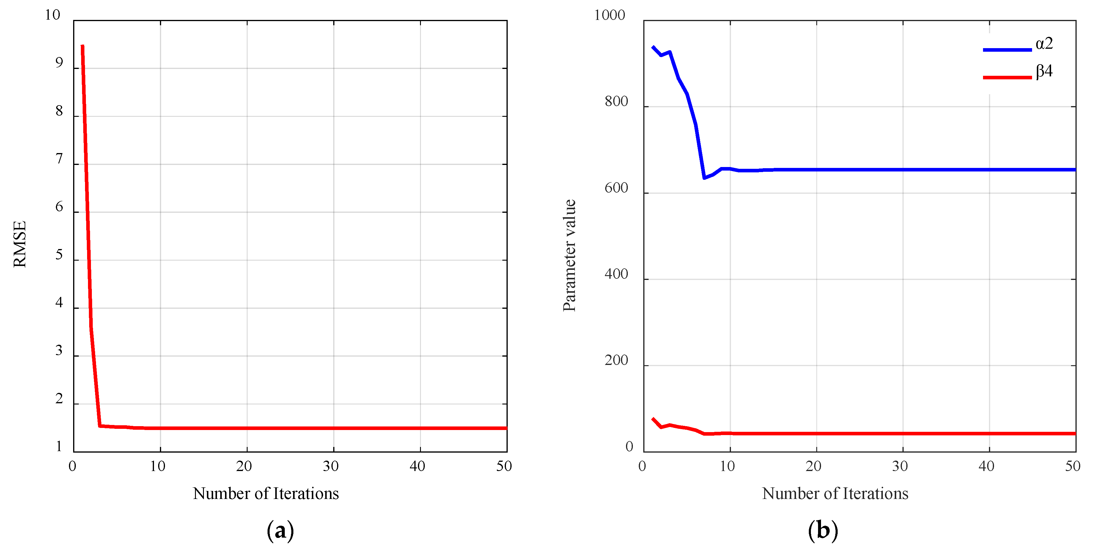
It can be seen from the identification results of the lowering transfer function (Figure 6) that the fitness function and all the parameters to be identified reach the final convergence value within no more than 10 iterations. At this time, the fitness function value (RMSE) was 1.611 mm, and the convergence speed was significantly improved compared with the lifting process. The convergence speed is noticeably faster than that for the lifting process, which is primarily attributed to the simpler model structure involving only two parameters to be identified, thus reducing the difficulty of the parameter optimization. Finally, the two model parameters of the lowering process are obtained as shown in Table 2.

In summary, with the increase in the number of iterations, the fitness function value and the parameters to be identified in the process of lifting and lowering can rapidly decline and quickly stabilize, indicating that the adopted optimization method can achieve convergence within a small number of iterations, and has good global search ability and convergence stability.

In addition, to further investigate the relative influence of individual parameters on model stability and accuracy, this study conducted a parameter sensitivity analysis based on the WOA optimization results. Specifically, after the parameters converged to the optimal solution, the average rate of change in the root mean square error (RMSE) of the model output was calculated in response to a small perturbation (±1%) applied to each parameter near its optimal value. A larger rate of change indicates that the model performance is more sensitive to that parameter. The analysis results show that the system gain for the lifting process (${\alpha }_1$), the system gain for the descending process (${\alpha }_2$), and the time constant (${\beta }_4$) are the most significant key parameters affecting the model’s performance. Among them, ${\alpha }_1$ directly determines the steady-state accuracy of the lifting process, while ${\alpha }_2$ and ${\beta }_4$ jointly govern both the steady-state and dynamic performance of the descending process. This conclusion provides a valuable reference for prioritizing parameters during subsequent controller design.

3.1.2. LSTM Neural Network Compensator Training

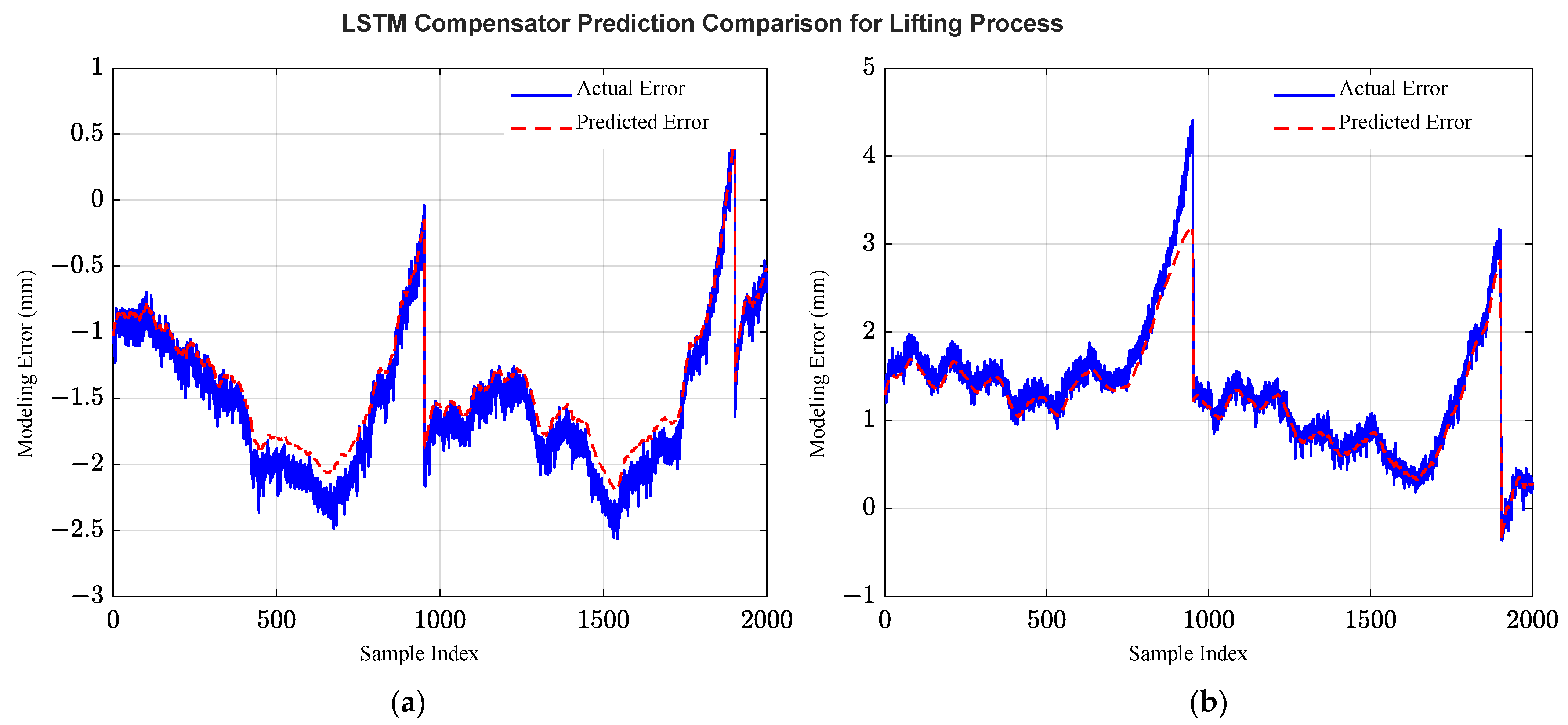
Based on the identification results of the above benchmark transfer function model, the test data are preprocessed to calculate the deviation between the output of the benchmark model and the measured system response. The processed data was divided into a training set (11,412 samples) and a validation set (3804 samples). The LSTM neural network compensator sample data was used for training. In order to facilitate visualization, Figure 7 and Figure 8 take 2000 samples as an example, and give the prediction error comparison results of the training set and the validation set of the lifting and lowering process, respectively.

The results show that the prediction error is basically consistent with the actual error change trend, indicating that the LSTM neural network model performs well under both working conditions. The statistical results of the lifting process are as follows: the RMSE, R² and MAE of the training set are 0.127 mm, 99.4% and 0.101 mm, respectively, and the RMSE, R² and MAE of the validation set are 0.138 mm, 99.7% and 0.110 mm, respectively. The statistical results of the lowering process are as follows: the RMSE, R² and MAE of the training set are 0.147 mm, 99.7% and 0.117 mm, respectively. The RMSE, R² and MAE of the validation set were 0.160 mm, 99.8% and 0.125 mm, respectively. It can be seen from the calculation results that the LSTM neural network compensator has high fitting accuracy for modelling errors under different working conditions, and the average prediction deviation is small.

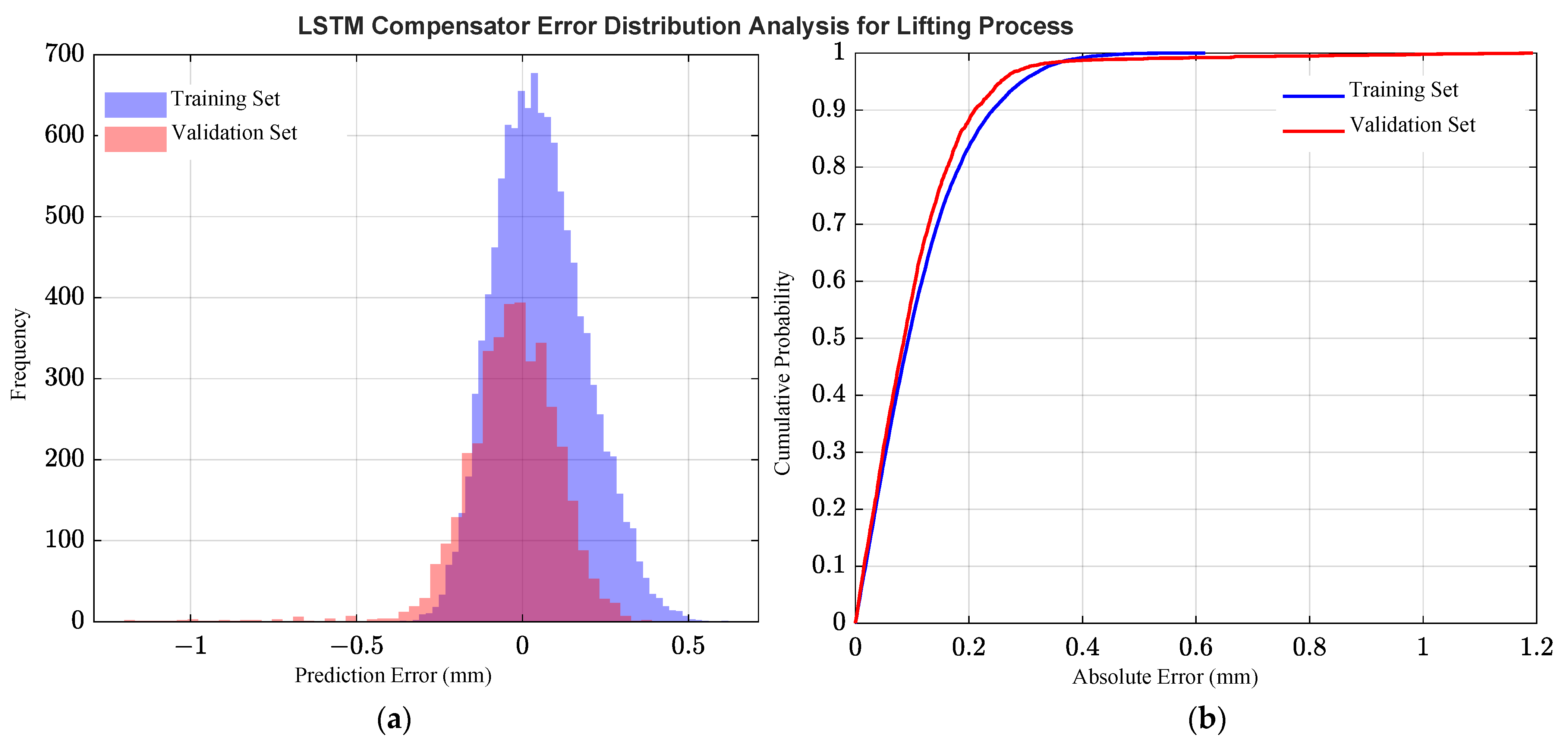
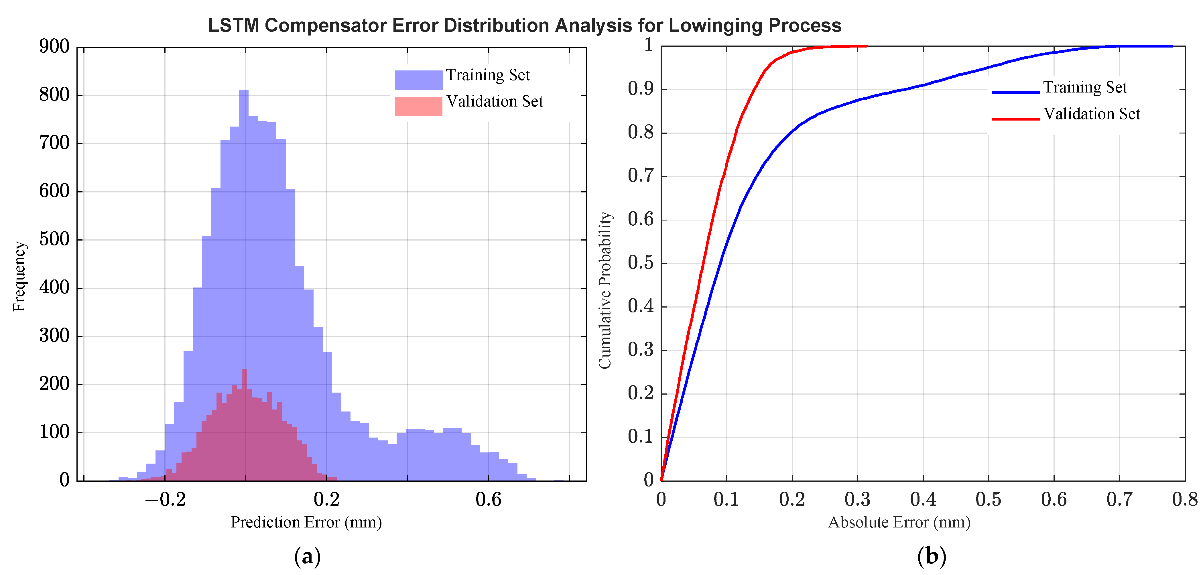
The prediction error distribution histogram and absolute error cumulative distribution curve of the lifting and lowering processes are shown in Figure 9 and Figure 10.

It can be seen from Figure 9a that the errors of the training set and the verification set of the lifting process are mainly concentrated in the range of ±0.2 mm. The overall error conforms to the normal distribution, and the model prediction results are stable. From the corresponding cumulative distribution curve (Figure 9b), it can be found that the absolute error of about 95% of the samples is less than 0.30 mm, which further verifies the stability of the model prediction results.

Compared with the results of the lifting process, the error distribution of the lowering process (Figure 10a) is relatively broad, and the training set is asymmetric. It shows that the prediction fluctuation of the model in the lowering process is slightly larger than that in the lifting process. However, the main error is concentrated between ± 0.2 mm, and the prediction accuracy is still at a high level. From the corresponding cumulative distribution curve (Figure 10b), it can be found that about 95% of the sample absolute error is less than 0.35 mm, which is not much different from the lifting process. It shows that the model has good stability in different stages of the system.

In summary, although the lowering and lifting processes show little difference in aggregated metrics such as RMSE and R², the secondary peaks in the error distribution reveal more complex dynamic characteristics. This phenomenon may be attributed to the physical nature of the lowering process, which is dominated by gravity: its dynamic response involves more severe discontinuous transients, such as static-to-dynamic friction transition. This results in more complex nonlinear dynamics than the pump-controlled lifting process, thereby posing a greater challenge to the accurate learning of the data-driven compensator.

3.2. Model Performance Validation

In order to verify the accuracy and generalization ability of the grey-box model, the test data independent of the model parameter identification sample dataset is used to test the grey-box model, and compared with the traditional single transfer function model.

3.2.1. Validation for the Lifting Process

The prediction results of the grey-box model and the single transfer function model established in this paper for the lifting process are shown in Figure 11

It can be seen from Figure 11a that the prediction results of the grey-box model are closer to the actual output, especially in the early and late time steps, the output of the transfer function model has obvious deviation. It can also be found from Figure 11b that in the whole process, the error of the transfer function model fluctuates greatly, and the error range is as high as 2.9 mm, while the overall error of the grey-box model is relatively stable and the fluctuation range is obviously small. From the perspective of the error distribution histogram (Figure 11c), the mean error distribution of the grey-box model is 0.21 mm, and the standard deviation is 0.24 mm. Although the centre is biassed towards the positive error, the overall distribution is more symmetrical. The mean error distribution of the transfer function model is 0.42 mm, and the standard deviation is 0.66 mm. The overall distribution is broad and not symmetrical; Through the cumulative distribution curve of absolute error (Figure 11d), it can also be found that about 98% of the samples in the grey-box model have absolute error less than 1 mm, while only about 79% of the samples in the transfer function model have absolute error less than 1 mm. The results of the grey-box model and the transfer function model were statistically calculated, and are presented in

Table 3. Modelling accuracy of the grey-box and transfer function models for the lifting processes.

Model Type	RMSE (mm)	MAE (mm)	R2
Transfer function	0.79	0.59	98.81
Grey-box	0.33	0.24	99.86

. The RMSE and MAE of the transfer function model of the lifting process are 0.79 mm and 0.59 mm, respectively. The RMSE and MAE of the grey-box model were 0.33 mm and 0.24 mm, respectively, which were 57.6% and 59.2% lower than those of the transfer function model. In summary, compared with the transfer function model, the grey-box model has stronger fitting ability, smaller error and more stable results in the lifting process.

3.2.2. Validation for the Lowering Process

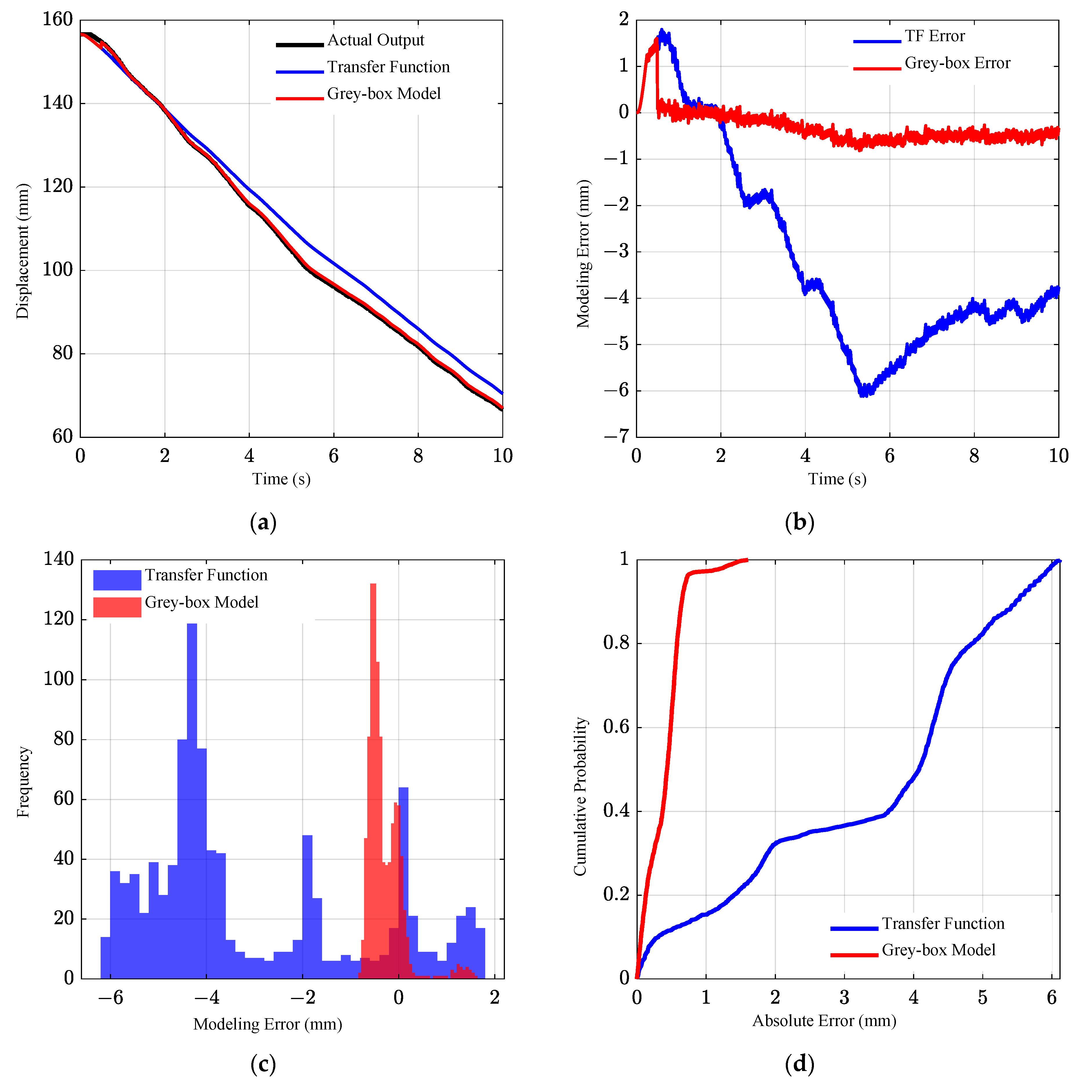
The prediction results of the grey-box model and the single transfer function model for the lowering process are shown in Figure 12.

It can be seen from Figure 12a that the grey-box model still has a good tracking effect during the lowering process, while the transfer function model has obvious deviation. From the comparison of modelling errors (Figure 12b), it can also be found that there are certain errors in the initial two models, but the grey-box model can quickly maintain stability, while the error value of the transfer function model increases rapidly, showing a large fluctuation, and the error range is as high as 7.6 mm. From the perspective of the error distribution histogram (Figure 12c), the mean error distribution of the grey-box model is 0.30 mm, the standard deviation is 0.38 mm, and the centre is biassed towards negative error, but the distribution range is narrow and the overall is symmetrical. The mean error distribution of the transfer function model is 3.06 mm, and the standard deviation is 2.24 mm. Compared with the lifting process, the overall distribution is wider and not symmetrical. It may be due to the simple lowering model, which cannot better describe the dynamics of the system. Through the absolute error cumulative distribution curve (Figure 12d), it can also be found that about 97% of the sample absolute error of the grey-box model is less than 1 mm, while the absolute error of the transfer function model is less than 1 mm. Only about 15% of the samples are less than 1 mm. The results of the grey-box model and the transfer function model are statistically calculated, and are presented in

Table 4. Modelling accuracy of the grey-box and transfer function models for the lowering processes.

Model Type	RMSE (mm)	MAE (mm)	R2
Transfer function	3.79	3.33	96.06
Grey-box	0.48	0.40	99.63

. The RMSE and MAE of the transfer function model of the lowering process are 3.79 mm and 3.33 mm, respectively. The corresponding indexes of the grey-box model are 0.48 mm and 0.40 mm, respectively, which are 87.3% and 87.9% lower than those of the transfer function model. In summary, compared with the transfer function model, the grey-box model still has stronger fitting ability, smaller error and more stable results in the lowering process.

4. Discussion

The grey-box model proposed in this paper achieves a significant improvement in accuracy compared to the traditional transfer function model. This improvement has a clear physical interpretation: it essentially reflects the capability of the constructed grey-box model to accurately describe nonlinear physical properties within the system. The traditional transfer function, being a linear model, cannot fully capture the complex nonlinear characteristics inherent in each process—such as the nonlinear flow gain and hysteresis of the proportional valve, as well as other unmodeled dynamics. In the proposed model, the LSTM neural network compensator is introduced to learn from data and compensate for the residuals of such linear models. On the one hand, the compensator’s ability to memorize historical states enables it to learn and predict dynamic errors caused by the hysteresis of the proportional valve. On the other hand, as a nonlinear autoregressive model, it inherently possesses the capacity to infer and fit unmodeled dynamics from time-series data. Therefore, the improvement in model accuracy is not merely a result of numerical optimization. The fundamental reason lies in the effective restoration, via data-driven compensation, of the nonlinear dynamics that cannot be represented by the linear transfer function model.

Compared with existing studies, the proposed method demonstrates comprehensive advantages in accuracy, efficiency, and structure. Reference [9], based on a purely mechanistic modelling approach, reports a deviation of 12.5% for the lowering process. References [15,17], respectively, employ pure black-box models based on TSFFCNN-PSO-SVM and NARX. Although these achieve high accuracy (99.37%) and R² = 96.04%, they suffer from limitations such as long training times (>2500 s) or lack of physical interpretability. In contrast, the grey-box model proposed in this paper achieves an R² of no less than 99.63% on the test set, with a total training time not exceeding 600 s. Its “mechanism-data” fusion architecture endows the model with clear physical interpretability while maintaining high accuracy, offering a more balanced and efficient modelling pathway for electro-hydraulic hitch systems. Furthermore, the high efficiency and precision demonstrated by this model also provide key feasibility for its extension to actual working conditions.

However, this method still has some limitations. On the one hand, the parameter identification process has a strong dependence on the sample data. When there is a large difference between the data and the sample due to the change in the working condition, the accuracy of the model prediction results may change. The primary reason is that, as a data-driven model, the generalization capability of the LSTM compensator is strictly constrained by the coverage and quality of the training data. Furthermore, the global search capability of the WOA used for benchmark model identification is achieved at the cost of high computational complexity. This not only explains why the proposed strategy employs offline identification but also limits its applicability in scenarios requiring fast online deployment. On the other hand, this paper is mainly based on offline data for parameter identification, and does not realize online adaptive adjustment of model parameters, which is still challenging in the face of complex field operation environment.

Future research will focus on the following aspects: First, online identification of the system model, combined with real-time data to adaptively estimate the system parameters; secondly, a more robust system model is established by considering the possible interference caused by complex working conditions in the field. Based on this, it provides more solid technical support for the intelligent control of tractor electro-hydraulic hitch system and the development of precision agriculture.

5. Conclusions

In this paper, the tractor electro-hydraulic hitch system has obvious asymmetry and strong nonlinear characteristics in the process of lifting and lowering. A distributed parameter identification method based on dual-mode grey-box modelling is proposed. The main conclusions are as follows:

(1)

Based on the mode decomposition strategy, the lifting and lowering processes of the electro-hydraulic hitch system were constructed into two subsystems, respectively, and the corresponding transfer function models were established. In order to improve the model’s ability to describe nonlinear systems, a LSTM neural network compensator is introduced to compensate the benchmark model, and a system grey-box model with both mechanism basis and high-precision characteristics was obtained, which effectively solves the problem that the dual-mode dynamic characteristics of the system are difficult to model uniformly.

(2)

Aiming at the high-dimensional and heterogeneous mixed parameter set in the established grey-box model, a distributed parameter identification strategy based on WOA and GD method was proposed to solve two complex joint optimization problems in a distributed manner, which effectively realizes the accurate identification of system model parameters.

(3)

The proposed grey-box model was verified by experiments. The results show that the RMSE of the model in the process of lifting and lowering were 0.33 mm and 0.48 mm, respectively, and the MAE were 0.24 mm and 0.40 mm, respectively. Compared with the single transfer function model, the accuracy of the model is significantly improved. This method can effectively improve the modelling accuracy of the system. It not only lays a reliable foundation for designing a high-performance controller for the tractor electro-hydraulic hitch system, but also provides a new paradigm for modelling a class of electro-mechanical–hydraulic systems with strong asymmetric and nonlinear dynamic characteristics.

References

1. Yang, Y.; Wen, Y.; Wang, R.; Dong, Z. A review of green agriculture and energy management strategies for hybrid tractors. Energies 2025, 18, 3224. [Google Scholar] [CrossRef]
2. Wang, L.; Wang, Y.; Dai, D.; Wang, X.; Wang, S. Review of electro-hydraulic hitch system control method of automated tractors. Int. J. Agric. Biol. Eng. 2021, 14, 1–11. [Google Scholar] [CrossRef]
3. Albiero, D.; Garcia, A.P.; Umezu, C.K.; Leme, R. Swarm robots in mechanized agricultural operations: A review about challenges for research. Comput. Electron. Agric. 2022, 193, 106608. [Google Scholar] [CrossRef]
4. Sunusi, I.I.; Wang, Z.Z.; Sun, C. Intelligent tractors: Review of online traction control process. Comput. Electron. Agric. 2020, 170, 105176. [Google Scholar] [CrossRef]
5. Aravind, K.R.; Raja, P.; Perez-Ruiz, M. Task-based agricultural mobile robots in arable farming: A review. Span. J. Agric. Res. 2017, 15, e02R01. [Google Scholar] [CrossRef]
6. Shen, W.; Wang, J.H.; Huang, H.L.; He, J.Y. Fuzzy sliding mode control with state estimation for velocity control system of hydraulic cylinder using a new hydraulic transformer. Eur. J. Control 2019, 48, 104–114. [Google Scholar] [CrossRef]
7. Tao, W.; Chen, B.; Yang, X.K.; Guo, B.; Xu, W.; Ke, S.; Huang, S.H. Design and experimental study of tillage depth control system for electric rotary tiller based on LADRC. Sci. Rep. 2025, 15, 1740. [Google Scholar] [CrossRef]
8. Wang, A.Z.; Ji, X.; Zhu, Y.Y.; Wang, Q.Z.; Wei, X.H.; Zhang, S.C. Tillage depth regulation system via depth measurement feedback and composite sliding mode control: A field comparison validation study. Meas. Control 2023, 57, 685–702. [Google Scholar] [CrossRef]
9. Kumar, S.; Tewari, V.K.; Bharti, C.K.; Ranjan, A. Modeling, simulation and experimental validation of flow rate of electro-hydraulic hitch control valve of agricultural tractor. Flow Meas. Instrum. 2021, 82, 102070. [Google Scholar] [CrossRef]
10. Hossain, M.S.; Sultan, I.; Phung, T.; Kumar, A. A literature review of the design, modeling, optimization, and control of electro-mechanical inlet valves for gas expanders. Energies 2024, 17, 4569. [Google Scholar] [CrossRef]
11. Yuan, H.B.; Na, H.C.; Kim, Y.B. Robust MPC-PIC force control for an electro-hydraulic servo system with pure compressive elastic load. Control Eng. Pract. 2018, 79, 170–184. [Google Scholar] [CrossRef]
12. Gao, Q.; Su, X.Y. An adaptive sliding mode controller for electro-hydraulic servo systems combining offline training and online estimation. Asian J. Control. 2024, 26, 1204–1218. [Google Scholar] [CrossRef]
13. Zhang, T.G.; Chen, G.X.; Yan, G.S.; Zhang, C.; Li, Y.; Ai, C. Research on the nonlinear characteristic of flow in the electro-hydraulic servo pump control system. Processes 2021, 9, 814. [Google Scholar] [CrossRef]
14. Nie, S.L.; Liu, Q.T.; Ji, H.; Hong, R.D.; Ma, Z.H. Prediction of degradation trend of water hydraulic high speed on/off valve based on machine learning. Chin. Hydraul. Pneum. 2022, 46, 60–66. [Google Scholar] [CrossRef]
15. Zhang, W.H.; Li, Z.Q.; Wang, P.F.; Liu, M.; Zhao, C.Y. Fault diagnosis of aircraft landing gear hydraulic system based on TSFFCNN-PSO-SVM. Chin. Hydraul. Pneum. 2024, 39, 20220111. [Google Scholar] [CrossRef]
16. Aela, A.M.A.; Jean-Pierre, K.; Mintsa, H. Adaptive neural network and nonlinear electrohydraulic active suspension control system. J. Vib. Control 2022, 28, 243–259. [Google Scholar] [CrossRef]
17. Gregov, G. Modeling and predictive analysis of the hydraulic geroler motor based on artificial neural network. Eng. Rev. 2022, 42, 91–100. [Google Scholar] [CrossRef]
18. Ülker, H. Design and application of an artificial neural network controller imitating a multiple model predictive controller for stroke control of hydrostatic transmission. Machines 2025, 13, 778. [Google Scholar] [CrossRef]
19. Eidin, A.; Youssef, R.; Ei-hamied, R. Mathematical models for predicating draft forces of tillage tools: A review. J. Adv. Agric. Res. 2021, 26, 48–52. [Google Scholar] [CrossRef]
20. Keleko, A.T.; Kamsu, B.; Ngouna, R.H.; Tongne, A. Health condition monitoring of a complex hydraulic system using deep neural network and deepshap explainable XAI. Adv. Eng. Softw. 2023, 175, 103339. [Google Scholar] [CrossRef]
21. Ma, Y.L.; Ye, M. Application of machine learning in hydraulic fracturing: A review. ACS Omega 2025, 11, 10769–10785. [Google Scholar] [CrossRef]
22. Ferrero, J.; Gomez, J.F.; Olivencia, F.; Crespo, A. A review of the use of artificial neural network models for energy and reliability prediction. a study of the solar PV, hydraulic and wind energy sources. Appl. Sci. 2019, 9, 1844. [Google Scholar] [CrossRef]
23. Cranmer, A.; Shahbakhti, M.; Hedrick, J.K. Grey-box modeling architectures for rotational dynamic control in automotive engines. In Proceedings of the 2012 American Control Conference (ACC), Montreal, QC, Canada, 27–29 June 2012; pp. 1278–1283. [Google Scholar] [CrossRef]
24. Obadina, O.O.; Thaha, M.A.; Mohamed, Z.; Shaheed, M.H. Grey-box modelling and fuzzy logic control of a Leader–Follower robot manipulator system: A hybrid Grey Wolf–Whale optimisation approach. ISA Trans. 2022, 129, 572–593. [Google Scholar] [CrossRef] [PubMed]
25. Karabacak, K. A grey-box model of a DC/DC boost converter for PV energy systems. Int. Trans. Electr. Energy Syst. 2024, 1, 3559456. [Google Scholar] [CrossRef]
26. Chen, Z.Q.; Kuang, F.J.; Yu, S.D.; Cai, Z.N.; Chen, H.L. Static photovoltaic models’ parameter extraction using reinforcement learning strategy adapted local gradient Nelder-Mead Runge Kutta method. Appl. Intell. 2023, 53, 24106–24141. [Google Scholar] [CrossRef]
27. Ahmadianfar, I.; Bozorg, O.; Chu, X.F. Gradient-based optimizer: A new metaheuristic optimization algorithm. Inf. Sci. 2020, 540, 131–159. [Google Scholar] [CrossRef]
28. Andersson, M.; Streb, M.; Ko, J.Y.; Klass, V.L.; Klett, M.; Ekstrom, H.; Johansson, M.; Lindbergh, G. Parametrization of physics-based battery models from input-output data: A review of methodology and current research. J. Power Sources 2022, 521, 230859. [Google Scholar] [CrossRef]
29. Liao, J.; Zhou, F.M.; Zheng, J.B. An improved parameter identification algorithm for the friction model of electro-hydraulic servo systems. Sensors 2023, 23, 2076. [Google Scholar] [CrossRef]
30. Lu, Z.; Zhao, S.Q.; Fan, Q.Q.; Zhu, X.D. A hybrid genetic algorithm-based parameter identification method for nonlinear hysteretic system with experimental verification. Int. J. Struct. Stab. Dyn. 2024, 24, 2450099. [Google Scholar] [CrossRef]
31. Zhou, S.; Wang, D.Z.; Ni, Y.L.; Song, K.L.; Li, Y.M. Improved particle swarm optimization for parameter identification of permanent magnet synchronous motor. CMC-Comput. Mat. Contin. 2024, 79, 2187–2207. [Google Scholar] [CrossRef]
32. Feng, W.; Zhang, W.J.; Huang, S.D. A novel parameter estimation method for PMSM by using chaotic particle swarm optimization with dynamic self-optimization. IEEE Trans. Veh. Technol. 2023, 72, 8424–8432. [Google Scholar] [CrossRef]
33. Zhao, C.; Li, X.J. Parameters’ identification of vessel based on ant colony optimization algorithm. Math. Probl. Eng. 2021, 2021, 6256785. [Google Scholar] [CrossRef]
34. Wang, M.; Chen, B.R.; Zhao, H.B. Data-driven rock strength parameter identification using artificial bee colony algorithm. Buildings 2022, 12, 725. [Google Scholar] [CrossRef]
35. Gao, K.Z.; Cao, Z.G.; Zhang, L.; Chen, Z.H.; Han, Y.Y.; Pan, Q.K. A review on swarm intelligence and evolutionary algorithms for solving flexible job shop scheduling problems. IEEE/CAA J. Autom. Sin. 2019, 6, 904–916. [Google Scholar] [CrossRef]
36. Li, Y.T.; Zeng, Y.; Qian, J.; Yang, F.J.; Xie, S.H. Parameter identification of DFIG converter control system based on WOA. Energies 2023, 16, 2618. [Google Scholar] [CrossRef]
37. Krainski Ferrari, A.C.; Gouvea da Silva, C.A.; Osinski, C.; Firmino Pelacini, D.A.; Leandro, G.V.; dos Santos Coelho, L. Tuning of control parameters of the whale optimization algorithm using fuzzy inference system. J. Intell. Fuzzy Syst. 2022, 42, 3051–3066. [Google Scholar] [CrossRef]
38. Li, C.J.; You, C.T.; Gu, Y.; Zhu, Y.F. Parameter identification of the RBF-ARX model based on the hybrid whale optimization algorithm. IEEE Trans. Circuits Syst. II Express Briefs 2024, 71, 2774–2778. [Google Scholar] [CrossRef]
39. Cui, X.S.; Guo, X.W.; Zhou, M.C.; Wang, J.C.; Qin, S.J.; Qi, L. Discrete whale optimization algorithm for disassembly line balancing with carbon emission constraint. IEEE Robot. Autom. Lett. 2023, 8, 3055–3061. [Google Scholar] [CrossRef]
40. Yang, G.Y.; Zhu, Q.J.; Wang, D.C.; Feng, Y.; Chen, X.X.; Li, Q.S. Method and validation of coal mine gas concentration prediction by integrating PSO algorithm and LSTM network. Processes 2024, 12, 898. [Google Scholar] [CrossRef]
41. Cui, Z.X.; Liu, H.C.; Yue, J.G.; Wu, C.H. TD-DALN: A twin data-driven design anomaly detection method for electrohydraulic actuators. IEEE Trans. Instrum. Meas. 2025, 74, 3508315. [Google Scholar] [CrossRef]
42. Song, Y.; Wang, S.J.; Wang, W.Q.; Wei, Q.; Zhang, J.M.; Tao, J.F. Response error prediction and feedback control method for electro-hydraulic actuators based on LSTM. Electronics 2025, 14, 1990. [Google Scholar] [CrossRef]
Figure 1. Working principle of the tractor electro-hydraulic hitch hydraulic system. 1. lifting cylinder; 2, 14. one-way valve; 3. lifting control valve; 4. damper; 5. throttle valve; 6. lowering control valve; 7. safety valve; 8. pressure compensation valve; 9. accumulator; 10. pressure gauge; 11. proportional solenoid-operated relief valve; 12. line filter; 13. high-pressure ball valve; 15. hydraulic pump; 16. electric motor; 17. suction filter; A. working port; T. return port; P. pressure port.
Processes 13 03608 g001
Figure 2. Overall structure of the tractor electro-hydraulic hitch system test bench.
Processes 13 03608 g002
Figure 3. Architecture of the system’s dual-mode grey-box model.
Processes 13 03608 g003
Figure 4. Strategy for distributed parameter identification.
Processes 13 03608 g004
Figure 5. Iteration curves during the lifting process: (a) Fitness function values; (b) Identified parameter values.
Processes 13 03608 g005
Figure 6. Iteration curves during the lowering process: (a) Fitness function values; (b) Identified parameter values.
Processes 13 03608 g006
Figure 7. Comparison of prediction errors during the lifting process: (a) Training set; (b) Validation set.
Processes 13 03608 g007
Figure 8. Comparison of prediction errors during the lowering process: (a) Training set; (b) Validation set.
Processes 13 03608 g008
Figure 9. Error distribution results during the lifting process: (a) Error distribution histogram; (b) Cumulative distribution of absolute errors.
Processes 13 03608 g009
Figure 10. Error distribution results during the lowering process: (a) Error distribution histogram; (b) Cumulative distribution of absolute errors.
Processes 13 03608 g010
Figure 11. Validation results for the lifting process: (a) Output signal comparison; (b) Modelling error comparison; (c) Error distribution histogram; (d) Cumulative distribution of absolute errors.
Processes 13 03608 g011
Figure 12. Validation results for the lowering process: (a) Output signal comparison; (b) Modelling error comparison; (c) Error distribution histogram; (d) Cumulative distribution of absolute errors.
Processes 13 03608 g012