Abstract
For extracting oil and gas from low-permeability reservoirs, pulse hydraulic fracturing offers superior performance over conventional hydraulic fracturing. Pulse hydraulic fracturing employs variable-rate injection to create pressure waves, which significantly increases the recovery rate. However, current pulse hydraulic fracturing research primarily focuses on the wellbore. The theory describing how pressure waves propagate and attenuate within fractures is still immature, potentially hindering the achievement of optimal fracture propagation and diversion. A two-dimensional pressure-wave equation incorporating both steady and unsteady friction was established and numerically solved using a high-accuracy explicit compact finite-difference method and was validated. The propagation process and pressurization phenomenon of pressure waves were analyzed, and the effects of treatment frequency, amplitude, and waveform, as well as steady and unsteady friction coefficients, on the attenuation characteristics of pressure waves within fractures were analyzed. The model’s validity is based on the pad fluid stage of hydraulic fracturing, informing the rational selection of treatment parameters in engineering practice, thereby improving fracturing performance and having practical significance for enhancing the development efficiency of low-permeability reservoirs.
1. Introduction
As global industrialization and urbanization accelerate, the demand for oil and natural gas continues to grow. However, as conventional oil and gas reserves diminish worldwide, oil and gas from low-permeability reservoirs are gradually becoming a key direction for industry development. Although they are difficult and costly to develop, they possess substantial development potential and abundant reserves. At present, the fracturing stimulation of low-permeability reservoirs relies mainly on conventional hydraulic fracturing. Conventional hydraulic fracturing uses surface constant-rate high-pressure pumps to inject low-viscosity fracturing fluid and proppant at high rates into the downhole completed interval, inducing fractures in the formation, removing near-wellbore damage, facilitating oil and gas entry into the production tubing, and increasing oil and gas production.
However, conventional hydraulic fracturing suffers from limited stimulation effectiveness [1]. In particular, when the horizontal principal stress difference is large, conventional hydraulic fracturing often creates only a single main fracture, failing to achieve the desired effect [2], thereby reducing the development efficiency of low-permeability reservoirs. As an emerging stimulation technique, pulse hydraulic fracturing (PHF) provides a solution to these shortcomings, wherein the fracturing fluid is injected into the formation as a dynamic load at a prescribed frequency using a pulse pump, or pulsed pressure waves are applied via a downhole pulse generator (Figure 1). As pressure waves propagate within artificial fractures, from the perspective of wave theory, they can produce reverberation, reflection, and superposition, resulting in a sharp increase in instantaneous peak pressure. From the perspective of rock mechanics, rocks subjected to pulsating loads undergo fatigue damage, which can reduce the fracture initiation stress and propagation pressure; the peak pressure acting on the reservoir during pulsed hydraulic fracturing increases substantially, facilitating the opening of a fracture network [3]. Most researchers have focused on the propagation mechanisms of pressure waves in the wellbore and on rock fatigue–damage mechanisms [4,5,6,7,8,9], whereas the key research questions concern the pumping pressure of the fracturing fluid and the propagation and attenuation of pressure within fractures. Few studies have investigated these topics. In particular, optimizing pulse parameters—on the basis of the amplitude and attenuation of pulse-pressure fluctuations—to achieve optimal fracture propagation and conductivity, and to convert stimulation outcomes into quantitative productivity predictions while verifying the effectiveness of the optimization scheme, hinges on establishing a reliable linkage between fracture performance and the reservoir productivity response. To meet this challenge, modern modeling approaches provide powerful tools. In this context, Lukin [10] developed the well–reservoir pseudo-connection model. In this pseudo-connection approach, the fracture plane is discretized into a series of additional well–reservoir connections where it crosses the grid, and each connection is assigned a time-varying transmissibility coefficient based on the fracture half-length, aperture (width), and conductivity; standard well inflow dynamic equations are then solved to obtain phase production rates and bottomhole flowing pressure, thereby enabling accurate simulation and evaluation of post-pulse hydraulic fracturing production dynamics.
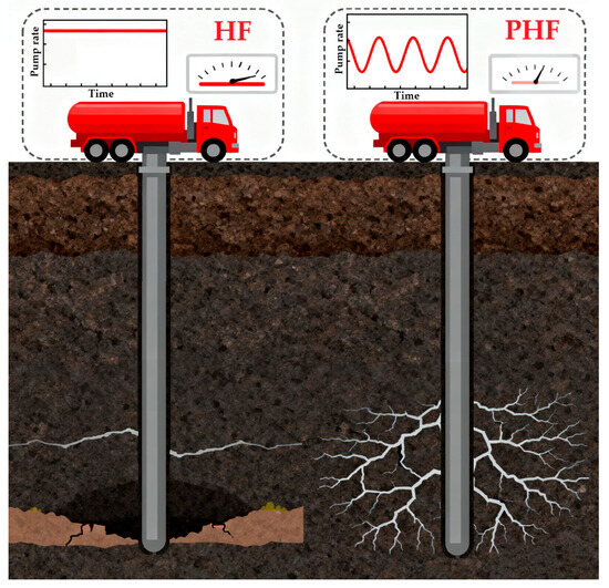
Figure 1.
Schematic comparison of conventional hydraulic fracturing (HF) and pulse hydraulic fracturing (PHF).
Current research on pressure-wave propagation in fractures can be classified into two main areas: experimental testing and numerical simulations.
Experimental research provides crucial support for validating the theoretical model and numerical simulation. Dyaur et al. [11] created a parallel-plate fracture model with two large acrylic plates (1 m length, 0.4 mm gap), and obtained the propagation characteristics of sinusoidal pressure waves in the model fluid. They found that at specific low frequencies, a transient pressure surge occurred, with the pressure inside the fracture 25.2 times the external pressure at 29 Hz. This was attributed to wave deceleration and accumulation effects in the thin fracture, consistent with numerical predictions.
Overall, experimental studies on pressure variations within narrow fractures have provided valuable insights. However, experiments often fail to account for the actual underground fracture dimensions and typically treat fractures as smooth, parallel plates, overlooking the effects of roughness and irregular deformation. Furthermore, they cannot investigate pressure-wave attenuation characteristics with friction as a variable. Additionally, for experimental rock samples or physical models, the pressure propagation cycle is on the millisecond scale, making monitoring extremely challenging, especially when accurately measuring pressure variations at different points within the fracture.
With the rapid development of computational fluid dynamics (CFD) technology, numerical simulation has become a key method in modern research.
Early numerical simulation mainly focuses on transient pressure variations in fractures beneath the lining slabs of stilling basins downstream of dams and on scour-induced failure of the bedrock foundations of high dams. Most researchers have conducted their studies on the transient flow model first proposed by Fiorotto et al. [12]. Liu [13] extended transient flow modeling to multi-stage planar fractures, revealing pulsed pressure hydraulic transients with evolving waveforms and frequencies. Stilling-basin experiments confirmed rapid pressurization, lagging peaks, and distance-attenuated amplitudes, validating the one-dimensional model. Wang and Li [14,15] innovatively applied the transient flow model to pulsed hydraulic fracturing; their results show that the fracture initiation pressure is 8 MPa—half that of conventional hydraulic fracturing—because frequency-doubling amplification occurs during pressure-wave propagation within fractures. They significantly advanced the fundamental theory of pulse hydraulic fracturing. Refs. [16,17,18,19,20] continued to use this model to study the fundamental patterns of pressure waves determined by fracture geometry, material properties, and fracture roughness. The results show that high-frequency components are significantly weakened by fracture roughness and infilling, while small fractures accelerate pressure attenuation, with faster decay observed in high-density rocks. The model was verified with experimental data and then applied to a broader range of application domains.
The transient flow model, while foundational for understanding pressure-wave propagation in fractures, exhibits important limitations in both theory and application. Existing research on wave behavior remains preliminary; although frequency and damping-induced attenuation is recognized, the underlying mechanisms and the influences of key parameters are poorly elucidated. Moreover, many studies overlook realistic geological conditions of low-permeability reservoirs as well as the role of fracture dimensions. Theoretically, the model simplifies multidimensional physical processes. In practical scenarios featuring wider fractures or three-dimensional flow characteristics—such as localized vortices and aperture variations—a one-dimensional representation becomes inadequate. Urbanowicz et al. [21] compiled eight experimental datasets and reported the mean absolute percentage error (MAPE) of pressure fluctuations for one-dimensional and quasi-two-dimensional transient flow models: in a turbulent-transient case, the pressure-amplitude error of the one-dimensional model exceeded 20%, and its late-time attenuation was insufficient, resulting in pressures approximately 12.5% higher than the measurements. In fact, steady friction in transient flow often overestimates the post-peak amplitude after pressure-peak decay. Studies [22] have indicated that, starting from the third peak, the amplitude deviation in steady friction simulations increases markedly. Therefore, in long-duration simulations of pressure oscillations, steady friction may cumulatively produce errors of several tens of percentage points, which is unfavorable to accurate engineering evaluation. Therefore, two-dimensional modeling and analysis are essential in pulse hydraulic fracturing research.
This study first established, through theoretical derivation, a two-dimensional pressure-fluctuation equation model that incorporates both steady and unsteady friction; a high-accuracy explicit compact finite-difference method was used to obtain the numerical solution of the model, and the accuracy of this method was verified. Further, the propagation of pulse pressure waves in fractures and the pressure-amplification phenomenon were investigated. The effects of pulse frequency, pulse amplitude, pulse waveform, and different types of damping coefficients on pressure were examined, as were the mechanisms of attenuation. This study helps engineers select appropriate implementation plans.
2. Pressure-Wave Equation Model
The evolution of mathematical models clearly reflects researchers’ relentless pursuit of a balance between computational efficiency and physical fidelity. According to the transient flow model proposed by Fiorotto [12], pulsed pressure propagates within fractures in the form of waves. Pressure waves have two functions: first, they can break blockages, clear fracture channels, and enhance fracture conductivity; second, they can induce dynamic redistribution of the internal stress field and cumulative fatigue damage in the rock mass, thereby reducing the breakdown pressure. The propagation and attenuation of pulsed pressure waves within fractures are influenced by multiple factors such as frictional resistance, frequency, amplitude, and other treatment parameters; therefore, selecting an appropriate mathematical model is crucial for investigating the mechanisms of pressure-wave propagation and attenuation.
2.1. Pressure-Wave Propagation Model
2.1.1. Seepage Model
Rehbinder [23] conducted studies on rock cutting by water jet. It was found that the fluid motion in this process primarily follows Darcy’s law, which is similar to the transmission of pulsed pressure within a single planar fracture, and can be expressed as:
where is the specific weight of the fluid; is the rock permeability; is the flow velocity within the fracture; is the horizontal distance along the fracture; is the fluid pressure. Since pulsed pressure mainly follows Darcy’s law, this model is suitable under conditions of severe blockage within the fracture.
2.1.2. Water-Hammer Model
The study by Zhao and Liang [24] demonstrated that when pulsed pressure is applied at both ends of a fracture, the fluid inside exhibits periodic oscillatory characteristics analogous to those of an incompressible fluid subjected to external forces within a circular pipe. Based on this theoretical model, the motion equation is expressed as:
where is the fluid density; is the fluid kinematic viscosity coefficient; is the flow velocity within the fracture; is the horizontal distance along the fracture; is the vertical distance across the fracture; and is the fluid pressure at a given point.
2.1.3. Transient Flow Model
Fiorotto [25] proposed a transient flow model, in which pressure transmission is not attributed to the macroscopic flow velocity of the fluid, but rather the fluid is regarded as a propagation medium for oscillatory waves, transmitting pressure disturbances through rock fractures in the form of waves. It is derived from the Navier–Stokes equations and simplified into a one-dimensional transient flow model, expressed as:
where is the fluid velocity within the fracture; is the propagation speed of the pressure wave, taken as 1000 m/s; is the resistance coefficient. is the damping term; is the fracture width; is the Darcy–Weisbach friction coefficient for the along-path resistance, which is closely related to the wall roughness of the fracture and the degree of blockage by the infilling materials.
The three models are compared below:
(1) The seepage model assumes a porous-medium framework with linear laminar flow governed by Darcy’s law and treats the rock mass as a permeable boundary; it is therefore not applicable to describing fluid flow in fractures.
(2) The water-hammer model is constructed on the basis of the water-hammer phenomenon in pipelines; it is better suited to cases in which all boundary conditions exhibit oscillatory variations and is therefore unsuitable for flow in fractures.
(3) The one-dimensional transient flow equation is derived from the continuity and momentum equations and accounts for steady friction. Compared with the preceding two models, it better captures the rapid transient pressure variations within fractures. Liu [26] verified this through simulations and experiments, showing that under complex pressure variations the transient flow equation yields the most accurate and reasonable results.
Building on the transient flow equation, this study establishes a two-dimensional pressure-fluctuation equation that incorporates unsteady damping.
2.2. Construction of the Unsteady Friction Pressure-Wave Equation Model
Since the disturbances in the fluid heat capacity and temperature gradient during pressure-wave propagation are relatively small, the process can be regarded as adiabatic; however, compared with an ideal gas, the adiabatic process of an ideal fluid medium is more complex. In the stationary state, the fluid possesses a static density . When a pressure wave passes through, the density becomes . Thus, the relationship between and satisfies . This isentropic relation can be obtained using the Taylor expansion:
where is the instantaneous pressure at position in the fluid; is the equilibrium pressure at that position; is the instantaneous density at position in the fluid; and is the equilibrium density at that position.
Since the density fluctuations caused by pressure-wave propagation are also small, the second- and higher-order terms in the Taylor expansion can be neglected; thus, the following linear relationship is obtained:
where: .
Since the compressibility coefficient is . Therefore, rearranging yields:
where is the fluctuating pressure at position in the fracture.
According to the continuity equation:
Therefore, we obtain:
Building on the transient flow model, we substitute the Darcy–Weisbach steady frictional resistance and the Brunone [27] unsteady frictional resistance into the Navier–Stokes equations:
According to the transient characteristics of pulsed pressure waves, it can be considered that: , ; , ; , . Therefore, Equation (9) is simplified to:
By taking the time derivative of the continuity equation, the divergence of Equation (10), and the time derivative of Equation (8), and then combining these three equations, we obtain:
By taking the partial derivatives of Equation (8) with respect to time and space, combining with Equation (11), and incorporating the continuity equation, rearranging yields the pressure fluctuation equation considering unsteady friction:
where is the fracture cross-sectional area; is the wetted perimeter; is the wave speed, defined as ; is the Darcy-Weisbach friction factor, with the expression: ; denotes the fracture roughness; denotes the Reynolds number; is the Brunone attenuation coefficient, where ; under laminar flow, = 0.000476, under turbulent flow, .
According to small density variations, the definition of the bulk modulus is:
The wave speed of the pressure wave is expressed as:
For the wave-speed coefficient in Equation (12), it is set as a wave-speed correction term; its physical meaning is that the wave speed in the fracturing fluid medium attenuates under the influence of unsteady along-path friction. For convenience of solution, this paper sets = . The above-derived equation is the two-dimensional pressure fluctuation equation for pulsed pressure waves, considering the steady along-path friction and unsteady along-path friction along the fracture.
2.3. Initial–Boundary Conditions and Numerical Simulation Parameters
The problem-defining conditions include the initial condition and the boundary condition. Boundary condition: the inlet boundary is specified as a pressure inlet to simulate the downhole pulse generator applying a pressure wave to the fluid within the fracture; the inlet pressure satisfies MPa. The fracture tip is a rigid and impermeable blind-end boundary. The wall boundary condition is set as a rigid, no-slip boundary. The numerical simulation parameters for pressure-wave propagation and attenuation within the fracture are as follows: the fracture model is 100 mm in length; the inlet width is 20 mm; the fracture-tip width is 4 mm. The initial conditions are as follows: the initial fluid velocity is 0 m/s, the holding pressure is 1 MPa.
3. Simulation Solution
The wave equation essentially belongs to the class of transient flow equations. The numerical solution can be obtained by various methods, such as the method of characteristics and the finite difference method. In this study, the numerical solution is obtained using an explicit compact finite difference scheme with sixth-order spatial accuracy and second-order temporal accuracy [28]. For the two-dimensional wave equation:
where is the wave speed; the domain is D = [x0,x1] × [y0,y1] = [0,L] × [0,]. In addition, the other functions , , , , , , are known and sufficiently smooth, and is the function to be solved.
Perform grid discretization by taking such that and , where denotes positive integers; is the spatial grid step, is the time step; the grid points are denoted by , where , , , , . Here, the high-order compact finite-difference scheme proposed by Lele [29] is adopted to obtain the numerical solution:
On both sides of the equation, perform a Taylor expansion about node :
the sixth-order accurate scheme is obtained:
First, compute the values of the second-order partial derivatives and then :
where: .
where .
For the boundary points:
where .
where .
Expand the first time point using the Taylor expansion:
Combining the initial conditions, we obtain:
As time advances, a central difference scheme is adopted:
Thus, an explicit compact scheme with sixth-order spatial accuracy and second-order temporal accuracy is obtained. The specific computational steps are as follows:
(I) Using Equation (15), compute the function values on the initial time level, and ;
(II) Let n = 1; using Equation (23), compute the function value on the first time level;
(III) Combine Equations (19) and (20) to compute the interior-node values and ; the boundary-node values are computed using Equations (21) and (22); compute the function value of at the n-th time level;
(IV) Using Equation (25), compute the function value at the n + 1-th time level;
(V) Let n = n + 1; repeat Steps (III) and (IV) until the time advances to the required instant for the computation and then terminate the calculation.
A mesh refinement study ensured a grid-independent solution, and the selected mesh satisfied numerical stability criteria; thus, the computational results are unaffected by temporal or spatial discretization errors (see Supplementary Materials for details). The calculation process is shown in Figure 2.
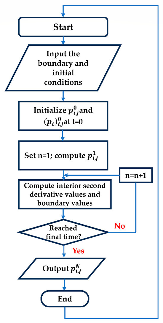
Figure 2.
Computational workflow diagram.
4. Results and Discussion
To simplify the analysis, unless otherwise specified, all formation and fracturing construction parameters in this chapter are taken from the tight sandstone reservoir of the second member of the Xujiahe Formation in the HC area of the Sichuan Basin [30]: the bottomhole construction pressure is 59.25 MPa; the mean minimum principal stress is 46.43 MPa; the mean maximum principal stress is 59.71 MPa. To obtain the influence of damping on pressure-wave attenuation under real conditions, a fracture model with a half-fracture length of 100 m and a width of 5 mm was established. Since a portion of the downhole construction pressure is used to overcome the confining stress of the surrounding rock to open and extend the fracture, a net pressure value of 8 MPa is adopted based on the literature survey. This study defines a reference pressure of 46.43 MPa, representing the system’s static ambient pressure. Throughout this paper, all reported pressures are expressed relative to this reference (gauge values), and the inlet boundary condition is set to + 5 MPa. The outlet boundary condition is 0 MPa (relative to the reference pressure). The fracture is filled with fracturing fluid at the initial time.
4.1. Accuracy Verification
This problem is solved using an explicit compact finite-difference scheme with sixth-order spatial accuracy and second-order temporal accuracy, while the conventional transient flow Equation (9) is solved using the method of characteristics; the results obtained by the two methods are compared.
It can be seen from Figure 3 that the results obtained by solving the wave equation with the high-accuracy finite-difference method and by solving the transient flow equations with the method of characteristics exhibit very small errors, with differences within 2%, which to some extent verifies the accuracy of the pressure-wave equation and computational method established in this paper. Considering that under high-frequency conditions or in complex flows within the fracture, the high-accuracy finite-difference method is more precise than the method of characteristics, the high-accuracy finite-difference method is therefore used subsequently.
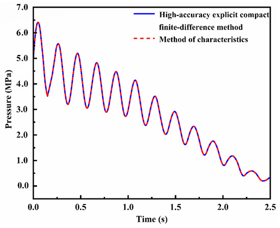
Figure 3.
Results of the method of characteristics and the high-accuracy finite-difference method (comparison of pressure attenuation curves along the fracture).
4.2. Pressure-Wave Propagation and Pressurization Phenomena Within the Fracture
Using the boundary and initial conditions given in Section 2.3, the problem is solved with the high-accuracy finite-difference method. A pressure with a peak value of 2 MPa is injected; the pulse frequency is 100 Hz; the time is divided into 1000 steps with a step size of 0.0001 ms. Seven cross-sections are set at the inlet, 25 mm, 50 mm, 60 mm, 70 mm, 90 mm, and 98 mm as monitoring sections, denoted as Inlet and A–F, respectively. Line plots of the pressure-wave propagation characteristics and velocity within the fracture are shown in Figure 4.
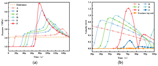
Figure 4.
Pressure and flow velocity versus time. (a) Pressure variation with time at different locations within the fracture; (b) Velocity curves of fracturing fluid within the fracture (characteristic line method).
From Figure 4 and Figure 5, the closer the fracturing fluid is to the fracture tip, the higher the peak pressure, because the pressure at the fracture front has undergone convergence and superposition, since the incident pressure wave forms an angle with the fracture wall, and the superposition of the blind-end reflected wave and the incident wave also produces a strong superposition effect in the tip region (Figure 6). In more detailed physical terms: because the fracture tip is a closed end, the fracturing fluid cannot discharge; the stationary fracturing fluid at the tip is compressed by the moving fracturing fluid behind it, leading to compression and an increase in density and pressure near the tip. When the fracturing fluid at a distance from the tip also comes to rest, it is likewise compressed by the fracturing fluid behind it, so the tip pressure reaches its maximum at 78 μs. Subsequently, after the fracturing fluid at a distance from the tip becomes stationary, it is again compressed by the fracturing fluid behind it, and so on, forming the well-known water-hammer effect—namely, the generation of an in-phase reflected pressure wave. If the leading end is closed, an in-phase pressure wave is produced and superimposes on the incident wave; if the leading end is open, an out-of-phase expansion wave is generated, which weakens the incident wave. Therefore, the water-hammer effect leads to energy concentration near the fracture tip. The peak pressure reaches three times the injection pressure; according to linear elastic fracture mechanics, if the stress intensity exceeds the critical value, i.e., the fracture toughness, the fracture will propagate further.
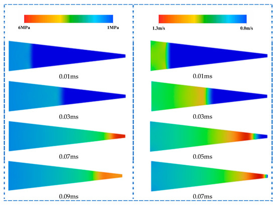
Figure 5.
Fracture internal pressure and velocity images. (a) Image of pressure-wave propagation within the fracture; (b) Image of fracturing fluid velocity variation within the fracture.
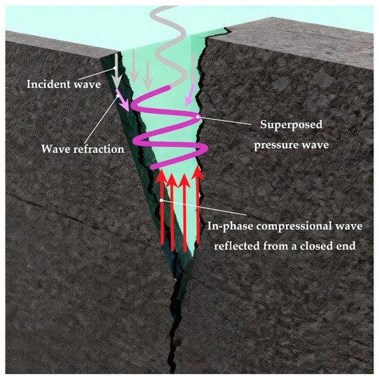
Figure 6.
Schematic of pressure-wave convergence, superposition, and amplification at a wedge-shaped fracture tip.
During the transmission of the first pressure wave, we can obtain the variation patterns of pressure and velocity. The influence on the fracturing fluid originates at the left inlet and gradually advances to the right; the region reached by the wave is a high-pressure zone: . The region not yet reached by the wave is a low-pressure zone: . At a certain instant, observe the fracture: taking as the dividing line the wavefront, i.e., the surface composed of points that the wave reaches after the same travel time in the fracturing fluid. The pressure decreases from the high-pressure region to the low-pressure region ; according to the definition of the pressure gradient, . Similarly, . For the continuity equation:
The blind-end boundary condition is:
To verify under one-dimensional conditions, at the fracture tip L:
Expanding the divergence term using the product rule of derivatives and substituting at, we obtain:
Since and , substituting into Equation (29) yields that the rate of change of density/pressure necessarily increases, and the fracture tip should satisfy the following rule: upon arrival of the incident wave: . After reflection, a phenomenon similar to water hammer occurs: .
4.3. Influence of Factors on Pressure-Wave Attenuation Within the Fracture
4.3.1. Analysis of Fracturing Fluid Pressure
In reality, pressure waves propagating in the fracture undergo attenuation due to the along-path friction. A 5 Hz sinusoidal injection pressure is prescribed, and using the high-accuracy explicit compact finite-difference method, the pressure distribution within the fracture as a function of time and fracture length is obtained, as shown in Figure 7:
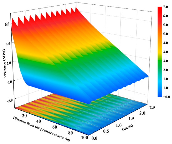
Figure 7.
Pressure variation with time and fracture length.
From Figure 7, it can be seen that as the pulsed pressure wave propagates within the fracture, its amplitude attenuates along the fracture length; however, how various parameters affect the transmission–attenuation process has not been elaborated in detail, leading to certain uncertainties and room for optimization in the control of pulse parameters in field applications.
4.3.2. Effect of Damping on Pressure-Wave Attenuation
Considering that the Brunone friction coefficient is generally small, the influence of unsteady friction on the pressure-wave velocity is ignored, and the wave velocity is assumed to be a fixed value of 1392 m/s. Using the single-variable method, the simulation schemes are shown in Table 1 and Table 2.

Table 1.
Experimental scheme for the effect of the Darcy–Weisbach friction factor on pressure waves.
Table 2.
Experimental scheme for the effect of the Brunone friction factor on pressure waves.
Figure 8 shows the variation in the pressure-wave amplitude with transmission distance for different steady friction coefficients. It can be seen that when the steady friction is zero, the pressure amplitude first increases and then rapidly attenuates. This is because, in the absence of friction, when the bottomhole treatment pressure exceeds the pressure at the fracture front and the system is at the critical state of extension, upon the arrival of the compression wave, a portion of the energy is used to extend the fracture; due to the pressure boundary condition, the pressure of the fracturing fluid at the front decreases, the density decreases, and an expansion wave with phase inversion—similar to the water-hammer phenomenon [31]—is generated. The phase difference causes the amplitudes of the compression wave and the expansion wave to superimpose at certain locations; in general, the amplitude is maximal at a distance of one-quarter wavelength from the front end. When the fracturing fluid is subjected to steady friction, the pressure-wave amplitude gradually decreases, exhibiting an approximately exponential decay trend; moreover, the greater the steady friction, the larger the attenuation rate of the pressure amplitude over 0–30 m. When the Darcy friction coefficient is 2, the pulse pressure amplitude is 0.63 MPa at 30 m and 0.15 MPa at 80 m, corresponding to 48.83% and 11.61% of the amplitude at 5 m, respectively. When the coefficient is 5, the amplitudes are 0.49 MPa at 30 m and 0.08 MPa at 80 m, which are 39.57% and 6.47% of that at 5 m. When the coefficient is 10, the amplitudes are 0.42 MPa at 30 m and 0.06 MPa at 80 m, corresponding to 35.29% and 5.57% of that at 5 m. This is because the initial flow velocity is high, and steady frictional resistance is proportional to the square of the velocity. Therefore, most of the mechanical energy is consumed in the near-wellbore region.
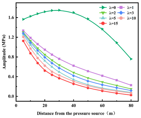
Figure 8.
Variation in pressure-wave amplitude with transmission distance under different steady friction coefficients.
Figure 9 shows the pressure amplitude versus position for different steady friction coefficients. It can be observed that the smaller the steady friction factor is, the weaker its effect on the attenuation of the pressure-wave amplitude. Conversely, a larger friction factor is typically associated with higher roughness of the fracture walls or the presence of obstructions, which significantly reduces the fracture conductivity and makes it difficult to maintain a sufficient pressure-wave amplitude at the far end of the fracture. Once the steady friction factor increases beyond a certain threshold, the pressure-wave amplitude no longer attenuates with distance.
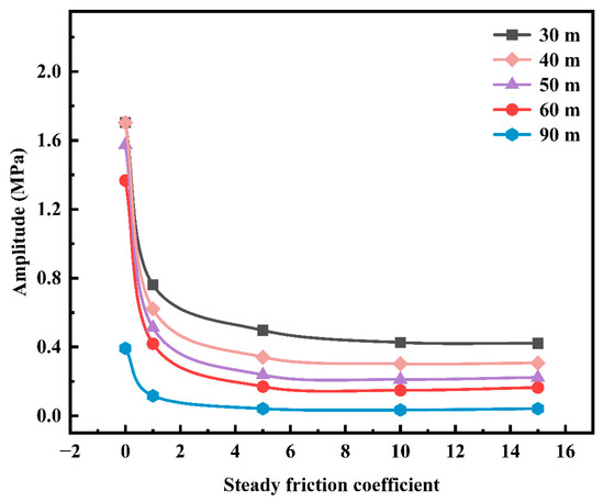
Figure 9.
Pressure amplitude versus position for different steady friction coefficients.
Figure 10 shows the pressure amplitude within the fracture under different non-steady friction coefficients. It can be seen that as the unsteady friction coefficient increases, the along-path amplitude of the pressure wave varies more markedly than under conditions considering only steady friction. Unsteady friction corrects the pressure through instantaneous acceleration and convective acceleration, better capturing the characteristics of transient flow and yielding more accurate results.
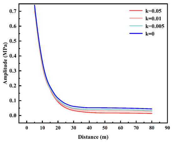
Figure 10.
Pressure amplitude within the fracture under different unsteady friction coefficients.
4.3.3. Effect of Frequency on Pressure-Wave Attenuation
To investigate the effect of different frequencies on pressure-wave attenuation, a single-variable approach is adopted; the simulation scheme is shown in Table 3.
Table 3.
Experimental scheme for the effect of frequency on pressure waves.
Figure 11 shows the result data under different frequency conditions. Timing and data acquisition commence after the pressure within the fracture has stabilized. In plotting Figure 11b, Y-axis values were offset to prevent overlap among the pressure-wave curves at different frequencies; the offset magnitude was determined by the pressure-wave amplitude. As the pulsing frequency increases, the along-path attenuation rate of the pressure-wave amplitude within the fracture increases accordingly; when the frequency exceeds 25 Hz, the pressure amplitude at 60 m is almost completely attenuated. When the frequency is 35 Hz, the pressure amplitude is attenuated by about 90% at 80 m of the crack. When the frequency is 50 Hz, the pressure amplitude at a distance of 80 m from the inlet has almost decayed to 0 kPa; therefore, selecting a high frequency cannot practically deliver the inherent advantages and intended effects of pulsed hydraulic fracturing.
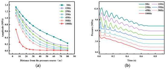
Figure 11.
The result data under different frequency conditions. (a) Along-path attenuation of pressure-waves amplitude in fractures under different frequency conditions; (b) Pressure attenuation curves along the fracture.
Based on the conclusion of Figure 8, the pressure wave attenuates more rapidly in the near-wellbore region; therefore, this study selects the location 5 m from the fracture inlet to investigate the mechanism responsible for the faster pressure-wave attenuation under high-frequency conditions. The influence of parameters on attenuation is characterized by the time-domain variation in the friction pressure drop per unit length (1 m) within the fracture. Figure 12a presents the specific values of the unsteady friction pressure drop at different frequencies. In plotting Figure 12, Y-axis values were offset to prevent overlap among the pressure curves at different frequencies; the offset magnitude was determined by the pressure amplitude. It can be seen that, under low-frequency conditions, the unsteady friction pressure drop is nearly zero and pressure attenuation is dominated by steady friction; with increasing frequency, the unsteady friction pressure drop strengthens markedly and exhibits pronounced oscillatory characteristics—at 35 Hz and above, its instantaneous peaks far exceed those at low frequency, and the fluctuations have larger amplitudes and higher frequencies, yielding larger-amplitude fluctuations in the unsteady friction pressure drop. This indicates that, during the propagation of pressure waves within the fracture, an increase in frequency significantly increases the unsteady frictional resistance.
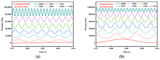
Figure 12.
The friction pressure drop values at different frequencies. (a) Unsteady friction pressure drop at different frequencies; (b) Steady friction pressure drop at different frequencies.
This is because unsteady friction is directly driven by the local acceleration of fluid micro-elements and the velocity gradient; the higher the frequency, the stronger the transient effects, and the greater the resulting unsteady resistance. Figure 12b presents the specific values of the steady friction pressure drop at different frequencies. Figure 13 shows the amplitude of the unsteady friction pressure drop at different frequencies. Figure 14 shows the amplitude of the steady friction pressure drop at different frequencies. It can be seen that the pressure amplitude of steady friction remains almost unchanged with increase in frequency, and the energy consumption of its single oscillation remains unchanged. However, the increase in the number of oscillations in the same time leads to faster continuous energy consumption, while the fluctuation amplitude of unsteady friction has a linear relationship with the increase in frequency. In physical terms, under high-frequency treatment conditions, the core flow velocity varies rapidly, preventing the boundary layer from fully developing. The no-slip boundary condition therefore yields a larger near-wall velocity gradient; according to Newton’s law of viscosity, the wall shear stress exhibits pronounced fluctuations that dissipate more energy. Moreover, high-frequency oscillations intensify turbulent fluctuations, increase the unsteady friction coefficient, and reduce the boundary-layer thickness, thereby increasing the degree of attenuation. In this case, the steady friction coefficient is 1 and the Brunone coefficient is 0.03. The following conclusions can be drawn: for larger steady friction coefficients, as the pulse frequency increases, pressure attenuation is dominated by the steady friction; for smaller steady friction coefficients, as the pulse frequency increases, pressure attenuation is dominated by the Brunone unsteady friction, because it increases linearly with frequency. The synergy of the two leads to the rapid attenuation of the amplitude of the continuous pulse pressure wave under high-frequency conditions.
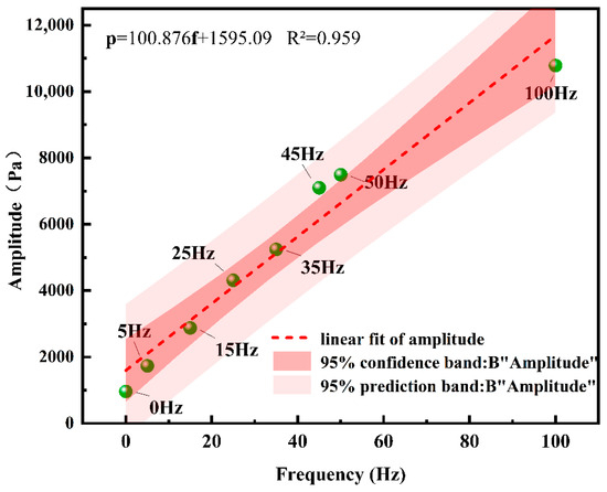
Figure 13.
The amplitude of the unsteady friction pressure drop at different frequencies.
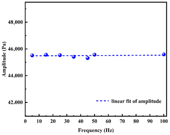
Figure 14.
The amplitude of the steady friction pressure drop at different frequencies.
Ni et al. [32], based on recent laboratory experiments, also found that when the pulsation frequency is 10–20 Hz, the compressive strength of core samples tends to decrease as the frequency increases; at 20 Hz, the compressive strength reaches its minimum, and when the pulsation frequency exceeds 20 Hz and continues to rise, the compressive strength remains nearly unchanged. When the pulsation frequency is 10–20 Hz, the amplitude attenuation rate exceeds 10%, and the effective propagation distance is approximately 100 m. This also demonstrates that employing high frequencies cannot achieve optimal results due to rapid attenuation.
In addition, according to resonance theory, pressure waves not only produce superimposed pressurization within the fracture but, under certain conditions, resonance pressurization may also occur when the injection frequency reaches the natural frequency of the fracture. It can be concluded that, in actual fracturing operations, there exists an optimal frequency for different formation conditions, which can significantly increase the pressure-wave amplitude within the fracture and result in slower attenuation. This study suggests setting the following: , where is the wave speed and is the main fracture length. However, field-scale fractures are not uniformly distributed, and such heterogeneity may significantly alter the resonance conditions. Therefore, achieving the so-called resonance condition is difficult; accordingly, this result is preliminary and requires further empirical evidence.
4.3.4. Effect of Amplitude on Pressure-Wave Attenuation
Under the 5 Hz condition, a low-viscosity fracturing fluid with a viscosity of 0.006 Pa·s, a density of 1135 kg/m3, and a wave speed of 1392 m/s is used, and injection amplitudes from 1.5 MPa to 5.5 MPa are employed for the calculations.
Figure 15 presents the attenuation curves of the pressure and pressure amplitude of the pressure wave with fracture length under different injection-pressure amplitudes. Figure 16 shows that increasing the injection amplitude markedly increases the steady friction pressure drop, whereas it has a much smaller effect on the unsteady friction pressure drop. It can be seen that selecting a higher injection amplitude can maintain a higher pressure within the fracture; Ni et al. [32] also found experimentally that the change in amplitude of low-frequency pulsating pressure is inversely proportional to the rock’s compressive strength. Therefore, in field applications, a higher injection amplitude should be selected within a reasonable range.
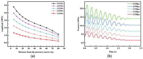
Figure 15.
Attenuation curves of pressure and pressure amplitude of the pressure wave with fracture length. (a) Pressure-amplitude attenuation curve; (b) Pressure attenuation curve.
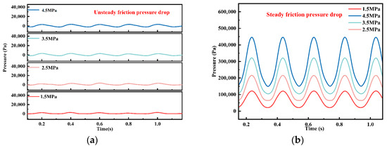
Figure 16.
The friction pressure drop values at different amplitude. (a) Unsteady friction pressure drop at different amplitudes; (b) Steady friction pressure drop at different amplitudes.
4.3.5. Effect of Pulse Type on Pressure-Wave Attenuation
Pulsed pressure waves with different waveforms exhibit their own unique characteristics during propagation, which directly influence the generation and propagation of fractures, as well as the placement, migration, and conductivity of proppants. Therefore, studying the impact of different pulse waveforms on pressure waves can provide more accurate technical support for pulsed fracturing operations, ensuring the maximization of construction effectiveness and safety. Sinusoidal, rectangular, and steady input pressures are employed, with a frequency of 15 Hz and an amplitude of 1.5 MPa; all other parameters are held constant.
Figure 17 illustrates the pressure variation at 90 m within the fracture under different input waveforms. It can be observed that, during the initial injection period, the pressure at this location experiences intense and complex fluctuations due to the superposition of reflected waves from the boundary and continuous pressure waves from the energy source, leading to significant pressure oscillations. Under constant injection pressure, the pressure stops fluctuating within 0.7 s and maintains the same waveform as the input pressure. The pressure stabilizes at 5 MPa. Under sinusoidal injection pressure, the pressure ceases its fluctuations within 1.3 s, maintaining the same waveform as the input pressure, with the maximum pressure before stabilization reaching 17 MPa and the maximum pressure after stabilization being 6 MPa. Under rectangular injection pressure, the pressure stops fluctuating within 16 s but does not maintain the same waveform as the input pressure. The maximum pressure before stabilization is 21 MPa, while the maximum pressure after stabilization is 12 MPa. This is because, during half of the input cycle, the rectangular injection pressure experiences a sharp change, resulting in a very large rate of change that leads to significant water-hammer effects, causing drastic pressure fluctuations. In this case, as defined in the introduction to Section 4, 21 MPa is a gauge pressure relative to the 46.43 MPa reference; the actual pressure is, therefore, 67.43 MPa (21 + 46.43 MPa), which is 4.2 times the pressure generated in conventional fracturing and 3.5 times that of the sinusoidal injection pressure. This demonstrates that the rectangular injection pressure, through water-hammer effects, has a highly positive influence on fracture propagation. It should be noted that this conclusion was derived for the pad fluid during the fracture initiation and propagation stages, and it does not consider proppant transport, the risk of sand plugging, or equipment fatigue. Therefore, this conclusion has corresponding limitations; its application should be regarded as a provisional understanding, and the above factors must be examined as key factors in subsequent comprehensive process analysis and practice.
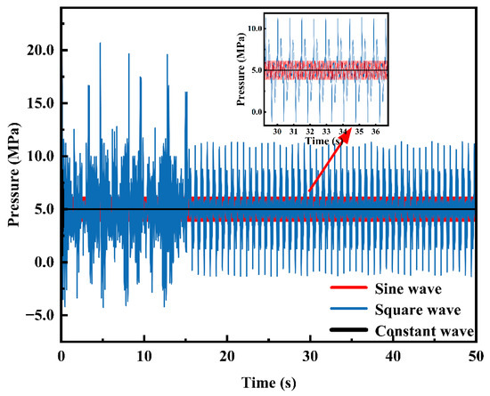
Figure 17.
Pressure variation at 90 m within the fracture under different input waveforms.
In conclusion, in the pulsed hydraulic fracturing process, the most significant factors affecting fracture propagation and the ultimate fracturing effectiveness are the treatment parameters and the friction of the fracture and the tubing. After the treatment parameters are optimized, an important factor is the magnitude of the along-path friction within the fracture, which governs the degree of pressure-wave attenuation in the fracture. Given that hydraulic fracturing is a complex process, these findings are preliminary and require additional empirical evidence. This study has certain limitations; for example, the conclusions were obtained for the pad fluid during the fracture initiation and propagation stages, and it does not consider fracture tortuosity or the rheology of the fracturing fluid, nor the effects of the proppant during the proppant-carrying fluid stage. Moreover, the stress sensitivity of the rock during pulsed fracturing may affect the pulse pressurization effect, and stress sensitivity is also an important factor to be considered in the next step. Therefore, investigating how to reduce the friction of the fracture and the tubing, and how fracture tortuosity and stress sensitivity affect pressure waves within the fracture, as well as research on the distribution and transport of proppant within the fracture under pulsing conditions, should become the main research directions for future pulsed hydraulic fracturing.
5. Conclusions
This study establishes a two-dimensional pressure-wave equation that takes into account unsteady friction to investigate the propagation and attenuation of pressure waves within fractures. The equation is solved using a high-accuracy finite-difference method, and the model demonstrates excellent correctness and high precision. Based on this model, the pressurization mechanism of pressure-wave propagation within the fracture, as well as the effects of frictional coefficients and construction pulse parameters on pressure-wave attenuation in the fracture, were analyzed.
Excessively high frequencies can cause rapid attenuation of pressure within the fracture. In field applications, to achieve the best fracturing effect, it is recommended to select a low pulse injection frequency (1–25 Hz). In the later stages of pulsed fracturing, after the main fracture has been formed, it is advised to set the pulse injection frequency to the resonant frequency of the tubing and the main fracture (including the length of the tubing and open-hole section) to facilitate the expansion of a complex fracture network.
In actual fracturing field applications, the frictional coefficient needs to be calculated based on flow patterns and empirical formulas. A higher frictional coefficient may indicate high roughness or severe blockages within the fracture, which may require wellbore cleanup measures.
The injection amplitude and waveform have a significant impact on pressure propagation and attenuation within the fracture. In actual fracturing operations, it is recommended to set the injection amplitude to the maximum value within the specified range. Setting the injection waveform to a rectangular shape can achieve better fracturing and production enhancement results.
The recommended ranges for optimal operational frequency, amplitude, and waveform in the above conclusions were derived from idealized simulations. Due to limitations of the experimental apparatus and other conditions, theoretical research on pulsed hydraulic fracturing is currently at an early stage. Therefore, prior to practical application, laboratory or pilot-scale tests are necessary to confirm its effectiveness and to evaluate the impacts of actual formation conditions and engineering complexity.
Supplementary Materials
The following supporting information can be downloaded at: https://www.mdpi.com/article/10.3390/pr13113513/s1, Table S1. GCI analysis.
Author Contributions
Conceptualization, methodology, software, writing—original draft preparation, Y.S.; validation, H.Z.; formal analysis, investigation, resources, data curation, writing—review and editing, H.Q.; visualization, Y.W.; supervision, project administration, funding acquisition, G.J. All authors have read and agreed to the published version of the manuscript.
Funding
This research was funded by the Foundation of Chongqing University of Science and Technology, grant number YKJCX2420123.
Data Availability Statement
The datasets in this paper are part of an ongoing study and are therefore not readily available. The raw data supporting the conclusions of this article will be made available by the authors on request.
Acknowledgments
Special thanks to the laboratory staff and technical team at the Institute of Unconventional Oil and Gas, Chongqing University of Science and Technology, for providing the experimental equipment essential to this work. We are grateful to all staff members and colleagues of the institute for their support. We also thank Jiahong Gou and Tao Li for providing the necessary equipment, resources, and assistance in conducting the experiments. We are also thankful to our colleagues and peers for their collaboration, helpful discussions, and moral support during the research. The funder had no role in the study design, data collection and analysis, interpretation of results, writing of the manuscript, or the decision to submit for publication.
Conflicts of Interest
The authors declare no conflicts of interest.
References
- Li, X. Study on Stimulation Mechanism of Energy Storage Volume Fracturing in Tight Sandstone Reservoir. Ph.D. Thesis, Northeast Petroleum University, Daqing, China, 2020. [Google Scholar]
- Miao, Z.; Wu, T.; Zhang, R. Numerical simulation of complex fracture-network formation in volume fracturing of tight oil reservoirs. Pet. Mach. 2022, 50, 96–102. [Google Scholar]
- Wei, C. Study on the mechanism of hydraulic fracture propagation and fracture network formation under pre hydraulic fracturing. Ph.D. Thesis, Shandong University, Jinan, China, 2022. [Google Scholar]
- Parchei-Esfahani, M.; Gee, B.; Gracie, R. Dynamic hydraulic stimulation and fracturing from a wellbore using pressure pulsing. Eng. Fract. Mech. 2020, 235, 107152. [Google Scholar] [CrossRef]
- Thomas, G.; Hough, D.; Shang, L.; Qian, S. Gas desorption characteristics effected by the pulsating hydraulic fracturing in coal. Fuel 1994, 236, 190–200. [Google Scholar]
- Cerfontaine, B.; Collin, F. Cyclic and fatigue behaviour of rock materials: Review, interpretation, and research perspectives. Rock Mech. Rock Eng. 2018, 51, 1–24. [Google Scholar] [CrossRef]
- Xie, J.; Xie, J.; Ni, G.; Rahman, S.; Sun, Q.; Wang, H. Effects of pulse wave on the variation of coal pore structure in pulsating hydraulic fracturing process of coal seam. Fuel 2020, 264, 15. [Google Scholar] [CrossRef]
- Zhao, A. Research on Fracturing Mechanism of Pulse Cycle Hydraulic Fracturing in Tight Reservoirs. Master’s Thesis, Northeast Petroleum University, Daqing, China, 2023. [Google Scholar]
- Hou, Y.; Peng, Y.; Chen, Z.; Liu, Y.; Zhang, G.; Ma, Z.; Tian, W. Investigation on the controlling factors of pressure wave propagation behavior induced by pulsating hydraulic fracturing. SPE J. 2021, 26, 2716–2735. [Google Scholar] [CrossRef]
- Lukin, O.; Kondrat, O. Utilizing well-reservoir pseudo-connections for multi-stage hydraulic fracturing modeling in tight gas saturated formations. Min. Miner. Depos. 2024, 18, 113–121. [Google Scholar] [CrossRef]
- Dyaur, N.; Jin, Y. Laboratory evidence of transient pressure surge in a fluid-filled fracture as a potential driver of remote dynamic earthquake triggering. Seism. Rec. 2021, 1, 66–74. [Google Scholar] [CrossRef]
- Fiorotto, V.; Rinaldo, A. Turbulent pressure fluctuations under hydraulic jumps. Hydraul. Res. 1992, 30, 499–520. [Google Scholar] [CrossRef]
- Liu, P.; Deng, X. Numerical study on pulse pressure propagation in multi-stage plate fractures. Chin. Theor. Appl. Mech. 1998, 30, 662–671. [Google Scholar]
- Wang, W.; Li, X.; Lin, B.; Zhai, C. Pulsating hydraulic fracturing technology in low-permeability coal seams. Int. J. Min. Sci. Technol. 2015, 25, 681–685. [Google Scholar] [CrossRef]
- Li, A.; Liu, P. Study on the attenuation mechanism of pulse pressure propagation in plate fractures. Water Resour. Hydropower Technol. 2006, 6, 33. [Google Scholar]
- Zhou, S. Study on the Pore Pressure Wave Propagation Law of Pulsating Water Flooding. Master’s Thesis, China University of Petroleum (East China), Qingdao, China, 2022. [Google Scholar]
- Li, X. The Mechanism and Technology of Permeability Enhancements in Coal Seam Based on High Pressure Pulsating Hydraulic Fracturing. Ph.D. Thesis, China University of Mining and Technology, Xuzhou, China, 2008. [Google Scholar]
- Zhang, J.; Zhou, Z. Propagation characteristics of pulse pressure in bottom plate fractures of water cushion ponds. Sichuan Univ. (Eng. Sci. Ed.) 2000, 3, 5–8. [Google Scholar]
- Wang, Y.; Zhang, J.; Xi, M.; Qu, J. Experimental study on propagation of flucturation pressure in fissures. Hydraul. Eng. 2009, 12, 44. [Google Scholar]
- Zhang, H.; Zhang, J.; Hu, B.; Zhu, F.; Zhang, N. Change of Medium Impact on Propagation Characteristic of Water. Coal Technol. 2014, 33, 26–29. [Google Scholar]
- Urbanowicz, K.; Andrade, D.; Kubrak, M.; Kodura, A. Accuracy and limitations of 1D and Q2D water hammer models for laminar and turbulent flows. J. Braz. Soc. Mech. Sci. Eng. 2025, 47, 666. [Google Scholar] [CrossRef]
- Abdeldayem, O.; Ferras, D. Analysis of Unsteady Friction Models Used in Engineering Software for Water Hammer Analysis: Implementation Case in WANDA. Water 2021, 13, 495. [Google Scholar] [CrossRef]
- Rehbinder, G. Slot cutting in rock with a high-speed water jet. Int. J. Rock Mech. Min. Sci. Geomech. Abstr. 1977, 14, 229–234. [Google Scholar] [CrossRef]
- Zhao, Y.; Liang, X. Investigation on Fluctuating Pressure Transmission along Joints. J. Tianjin Univ. 1988, 3, 55–65. [Google Scholar]
- Fiorotto, V.; Rinaldo, A. Fluctuating uplift and lining design in spillway stilling basins. J. Hydraul. Eng. 1992, 118, 578–596. [Google Scholar] [CrossRef]
- Liu, P.; Li, A. Model discussion of pressure fluctuations propagation within lining slab joints in stilling basins. J. Hydraul. Eng. 2007, 133, 618. [Google Scholar] [CrossRef]
- Brunone, B.; Karney, B.W.; Mecarelli, M.; Ferrante, M. Velocity profiles and unsteady pipe friction in transient flow. J. Water Resour. Plann. Manag. 2000, 126, 236–244. [Google Scholar] [CrossRef]
- Sun, Y.; Song, L.; Ai, X. High-order compact explicit difference scheme for two-dimensional wave equation and stability analysis. J. Harbin Univ. Sci. Technol. 2024, 29, 141–148. [Google Scholar]
- Li, J.; Chen, Y.; Liu, G. High-order compact ADI methods for parabolic equations. Comput. Math. Appl. 2006, 52, 1343. [Google Scholar] [CrossRef]
- He, J.; Cao, F.; Deng, H.; Wang, Y.; Li, Y.; Xu, Q. In-situ stress evaluation of the Xushier tight sandstone reservoir in the HC area of the Sichuan Basin and its application in tight gas development. Geol. China 2023, 50, 1107–1121. [Google Scholar]
- Li, X. Understanding and practice of water hammer prevention in pressure pipeline engineering design. Chem. Eng. Des. Commun. 2020, 46, 81–82. [Google Scholar]
- Ni, W.; Yang, G.; Liu, G.; Fan, C.; Xie, C. Parameter optimization and field application of downhole low-frequency pulsation hydraulic fracturing technology. J. Earth Sci. Environ. 2023, 45, 643–652. [Google Scholar]


Disclaimer/Publisher’s Note: The statements, opinions and data contained in all publications are solely those of the individual author(s) and contributor(s) and not of MDPI and/or the editor(s). MDPI and/or the editor(s) disclaim responsibility for any injury to people or property resulting from any ideas, methods, instructions or products referred to in the content. |
© 2025 by the authors. Licensee MDPI, Basel, Switzerland. This article is an open access article distributed under the terms and conditions of the Creative Commons Attribution (CC BY) license (https://creativecommons.org/licenses/by/4.0/).