Abstract
Driven by the dual-carbon goals, photovoltaic (PV) battery systems at renewable energy stations are increasingly clustered on the distribution side. The rapid expansion of these clusters, together with the pronounced uncertainty and spatio-temporal heterogeneity of PV generation, degrades battery utilization and forces conservative dispatch. To address this, we propose a “spatio-temporal clustering–deep estimation” framework for short-term interval forecasting of PV clusters. First, a graph is built from meteorological–geographical similarity and partitioned into sub-clusters by a self-supervised DAEGC. Second, an attention-based spatio-temporal graph convolutional network (ASTGCN) is trained independently for each sub-cluster to capture local dynamics; the individual forecasts are then aggregated to yield the cluster-wide point prediction. Finally, kernel density estimation (KDE) non-parametrically models the residuals, producing probabilistic power intervals for the entire cluster. At the 90% confidence level, the proposed framework improves PICP by 4.01% and reduces PINAW by 7.20% compared with the ASTGCN-KDE baseline without spatio-temporal clustering, demonstrating enhanced interval forecasting performance.
1. Introduction
Driven by the “dual-carbon” goal, photovoltaic energy is transitioning from a supplementary source to a baseload supplier; however, its inherent variability and uncertainty impose multiple pressures on power systems with high renewable penetration—peak shaving, frequency regulation, and spot-market clearing among them. Accurately depicting the evolution trend of PV power has therefore become a critical issue for dispatch and operation [1]. Yet photovoltaic generation is subject to weather-induced uncertainty and randomness, threatening the stability of the electricity supply. Hence, accurate PV power forecasting is essential for enhancing photovoltaic accommodation by the power system.
Photovoltaic power forecasting is conventionally divided—by temporal horizon—into ultra-short-term [2], short-term [3,4] and medium- to long-term [5] categories, while spatially it spans distributed, single-plant, and cluster scales [6,7,8]. Cluster-level forecasts directly support regional dispatch: by “clustering first, aggregating later”, spatial complementarity can be exploited without extra hardware investment, improving observability and predictability [9,10,11]. Weather variability, however, may mislead dispatch decisions. Correlation-based selection of key Numerical Weather Prediction (NWP) features and fuzzy C-means (FCM) clustering into sunny, cloudy, and rainy regimes [12,13] improves accuracy, but is still limited by NWP’s inability to capture second-scale cloud transients. Clustering PV power directly and forecasting each type separately can reduce prediction error and mitigate random fluctuation. K-means, a popular algorithm, partitions data into K pre-defined cells [14,15], yet requires computable means, often converges to local optima, and is sensitive to initial centers. In contrast, K-Modes [16] uses category matching instead of Euclidean distance, making it naturally suited to discrete meteorological-power features (cloud cover, weather type) while remaining insensitive to initialization.
PV forecasting is generally cast into two output paradigms: point and interval prediction. Point forecasts deliver a single deterministic power value for each future instant, but they cannot quantify uncertainty and therefore struggle to support stochastic scheduling in systems with high PV penetration [17]. Yet PV output is highly volatile and strongly weather-driven, so a crisp point value offers little information on sudden ramps. Recent deep-learning models exploit large datasets to mine complex spatio-temporal patterns in an end-to-end manner; TCN [18,19], CNN [20], LSTM [21], and GRU [22] architectures are widely used to capture temporal and spatial dependencies. Reference [23] goes one step further and proposes a multi-graph spatio-temporal graph convolutional network (GCN) that constructs adjacency via the Euclidean distance between plants, markedly improving deterministic accuracy. Its graph structure, however, is fixed, ignores errors induced by modeling assumptions and data noise, and yields only a single value, leaving predictive uncertainty uncharacterized. Interval forecasting, in contrast, provides upper and lower power bounds at a prescribed confidence level. As an extension of point prediction, it covers the uncertain range of PV output more comprehensively [24]. Obtaining such intervals requires the probability distribution of forecast errors. Parametric estimation [25] demands an a priori distributional form, but the error distribution of PV forecasts is unknown and time-varying; a misspecified model can seriously degrade reliability. Non-parametric estimation [26] needs no prior, adapts to any density, and offers greater robustness and generalization; it has been successfully applied in many fields [27]. Among non-parametric techniques, kernel density estimation (KDE) [28] stands out for its well-established theory and ease of implementation, and has become the preferred tool for reconstructing error distributions and generating probabilistic or interval forecasts.
To address the above challenges, this paper proposes an ASTGCN-based short-term interval forecasting framework for PV clusters, targeting 20 PV plants in Jilin Province. The key steps are as follows:
- (1)
- In the day-ahead stage, a CNN is first employed to capture the power-fluctuation profile and produce a preliminary output trajectory. The forecasted power is then classified according to weather fluctuation types. By simultaneously considering the spatial and temporal characteristics of each plant, K-Modes clustering is applied to group stations with similar meteorological and generation patterns into one sub-cluster, smoothing intra-cluster prediction errors and making training samples more representative, thereby significantly improving overall accuracy.
- (2)
- Taking the sub-cluster topological graph as basic nodes, edge weights are dynamically learned from the real-time correlation coefficient and the geographical distance between plants. An ASTGCN is adopted to perform point forecasting for each sub-cluster, and the cluster-wide power prediction is obtained through cumulative fusion.
- (3)
- The point forecasts are finally fed into a KDE model to generate probabilistic intervals for the PV cluster, meeting the security and economic requirements of power systems with high-penetration PV-plus-storage.
- (4)
- The proposed method is compared with several alternatives, and additional experiments on PV clusters in other regions are conducted to verify its superiority and generalizability.
2. Photovoltaic Power Fluctuation Division
2.1. CNN-Based Preliminary Prediction of PV Power
CNN is one of the flagship algorithms of deep learning. The network architecture extracts the relevant features from the input data and, under the prescribed rolling window, performs recognition of these features.
CNN models are good at outputting high-dimensional data and do not require manual feature selection, can automatically classify and obtain good feature classification results, and have a powerful ability to extract input depth features. Using CNN as an accurate prediction model for PV power plants is often accompanied by a lot of pre-processing data work. Therefore, CNN models are more suitable for capturing PV power fluctuations. In this study, we use a CNN, which is mainly used for extracting image features, for preliminary prediction before PV power generation day, which can give a preliminary understanding of the power fluctuation. The predicted power is also typed for weather fluctuations to make it more relevant to train the prediction model and improve the prediction accuracy.
2.2. Fluctuation Classification Based on CNN-Derived Forecasted Power
Affected by meteorological factors, the training data quality is poor, and ultra-short-term power fluctuations are highly diverse. Figure 1 shows the power profile of a Jilin PV plant over one week: under the influence of irradiance, cloud cover, temperature, and wind speed, the output sometimes fluctuates violently within a single day with no clear trend, while at other times it remains smooth. Classifying the forecast data by weather type—grouping days with similar fluctuation behavior and training/predicting them separately—can significantly improve accuracy.
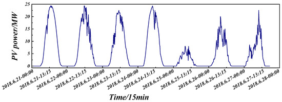
Figure 1.
Fluctuation curves of PV power output from a photovoltaic plant over one week.
Most existing studies [17] cluster weather types according to “fluctuation features” derived from NWP. Yet NWP is itself a forecast product with limited accuracy, and the irradiance and cloud-cover fields delivered by conventional meteorological stations are usually smoothed, lacking pronounced and high-frequency variability. More critically, high-quality measured PV data are both costly and difficult to obtain in advance. Using predicted power as the basis for weather typing is therefore more practical.
Figure 2 simultaneously plots the actual power, CNN-predicted power, and NWP-provided irradiance for a three-day summer rainy episode. Although NWP irradiance exhibits the same diurnal cycle as PV output, it rises and falls monotonically with solar elevation and shows no marked fluctuation when real power varies sharply because of weather disturbances. Consequently, weather typing based solely on NWP features is problematic. In contrast, a CNN trained on historical PV power together with NWP variables can learn these fluctuation patterns, capturing the stochasticity and uncertainty inherent in real plant operation.
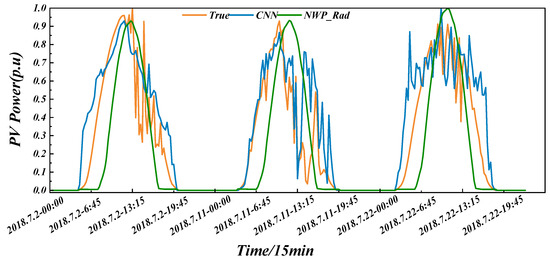
Figure 2.
Comparison of predicted power with actual power and irradiance.
2.2.1. Classification of Fluctuating Power Based on the Quadrature Method
Day-ahead PV power forecasts are first generated by a CNN, after which the forecast sequences are classified into complex-fluctuation and simple-fluctuation regimes to improve the congruence between training and test partitions. A fluctuation event is defined as the absolute difference between two consecutive forecast values exceeding a predefined threshold. Partitioning the series according to the fluctuation process rather than to static weather labels yields subsets with more distinct statistical signatures, which enhances the accuracy with which the deep-learning model learns the mapping from NWP variables to PV power.
Because complex and simple fluctuations differ markedly in volatility and stochasticity, and because simple patterns exhibit stronger regularity, the two regimes are trained separately, significantly improving the model’s ability to track contrasting fluctuation dynamics. The overall partitioning procedure is illustrated in Figure 3.
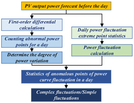
Figure 3.
The process of dividing PV power fluctuations based on the quartile method.
- 1.
- Outlier-fluctuation criterion
The day-ahead PV power series is first-order differenced to obtain sequence ; outliers in are detected by the inter-quartile method, and the daily count of points exceeding the quartile threshold is recorded. The detailed calculation is as follows:
In the equation, and denote the lower and upper thresholds of the first-difference fluctuation parameter, respectively; is the first quartile, the third quartile, and the inter-quartile range. A counter function is used to tally the number of fluctuations.
where is an indicator function that equals 1 when the condition is satisfied and 0 otherwise, and = 1.
- 2.
- Extreme-value fluctuation criterion
The number of daily extreme points, , in the forecast power series is counted to form sequence . The upper-quartile threshold of is then obtained by the inter-quartile method. The extreme-value calculation is as follows:
where is the observation at time i, and are the lower and upper thresholds of the first-difference extreme-value parameter, is the first quartile, is the third quartile, is the inter-quartile range, and the logical NOT ¬(·) indicates that the peak condition is not satisfied.
- 3.
- Fluctuating-weather identification
and as the upper quartile of and , the classification of complex fluctuating weather and simple fluctuating weather can be performed. When and , the power fluctuation is large, and it is judged as complex fluctuation type; when only one condition is satisfied or neither of them is satisfied, it is a simple weather type.
2.2.2. Fluctuation-Power Classification Results
The experimental data used in the case study come from a 20 MW PV power station in Jilin Province, covering the period from 2017 to 2018 with a sampling interval of 15 min. In this chapter, a CNN model is first trained using the entire year of 2017 as the training set to perform day-ahead PV power forecasting for 2018. The inputs to the CNN model include historical PV power data from 2017 and meteorological variables such as cloud cover and solar irradiance provided by NWP. The output is the forecasted PV power for 2018. Based on the day-ahead forecasted power, a quartile-based method is applied to classify the data into two weather types: fluctuating and simple.
The day-ahead forecasted power is normalized and, by counting daily power-fluctuation statistics, days are classified as either “fluctuating” or “simple”; quartile-based outlier analysis yields thresholds of [−2.61, 2.51] for the first-difference normal band, with first-difference upper-quartile = 1 and fluctuation upper-quartile = 19. After computing the first-difference series of the CNN-forecasted 2018 power, any value outside [−2.61, 2.51] is flagged, and a day is labeled “fluctuating” only if it contains more than 9 first-difference outliers and more than 19 power-fluctuation outliers, while all other days are labeled “simple.” Under this rule, 2018 has 113 complex-fluctuation days and 252 simple days; as shown in Figure 4, the proposed classification scheme effectively extracts highly variable weather, whose power profile is far more random and volatile than that of simple days. Training the two types together would allow the violent fluctuations of variable days to contaminate the smooth traits of simple days, and the uniform character of simple days would hinder the model from learning the instability inherent in variable-day PV output, underscoring the necessity of separate training and forecasting for simple and fluctuating weather.
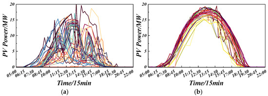
Figure 4.
Power curves for complex/simple weather types. (a) Complex-fluctuation weather type. (b) Simple weather type.
3. Clustering and Classification of PV Plants Considering Multiple Spatial and Temporal Scales
3.1. Spatial and Temporal Correlation of Photovoltaic Power Plant Cluster Classification
Figure 5 depicts the normalized power and irradiance profiles from 06:00 to 18:00 on a single day for twenty PV plants within one cluster. Although the plants lie in the same macro-region, climate and geographical differences induce pronounced disparities in power fluctuations. Even neighboring stations exhibit distinct profiles because slight cloud movements, panel orientations, and tilt angles produce dissimilar irradiance patterns. Consequently, the NWP-based feature set of a PV cluster tends to be complex, disorderly, and hard to predict, hindering model learning and degrading interval-forecast accuracy. To address this issue, we propose cluster partitioning: plants with similar spatial and meteorological traits are grouped into homogeneous sub-clusters, allowing targeted interval forecasting within each coherent sub-region.
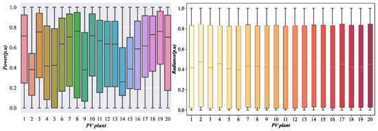
Figure 5.
Box line diagram of the power division of 20 PV plants for a certain day.
Differences in the power distribution of clustered PV plants arise mainly on temporal and spatial scales. Temporally, varying weather, wind speed, and direction drive cloud movement; the area and thickness of clouds above each plant determine the solar irradiance it receives and thus its output. Because the weather is highly changeable, PV power fluctuates accordingly. Days with rapid meteorological variations are therefore defined as “fluctuating weather”, while those with slow changes are termed “simple weather”. The number of fluctuating-weather days at a plant reflects the intensity of its power variability over the period.
NWP provides many meteorological variables, but their influences on cluster-wide power differ. We thus use correlation coefficients to select the weather features most strongly linked to power output; the inter-feature influences are illustrated in Figure 6.
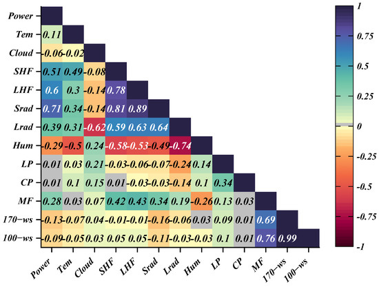
Figure 6.
Heatmap of Correlation Coefficients.
Through correlation analysis, we utilize cloud cover, irradiance, wind speed, temperature, and wind direction provided by NWP as primary meteorological features. Together with historical PV power and the number of days with volatile weather, these factors serve as criteria for partitioning. This approach enables the connection of photovoltaic stations experiencing similar weather conditions over a certain period of time.
From a spatial perspective, stations inside a large-scale photovoltaic base are geographically close, experience nearly identical meteorological forcings and land-surface characteristics, and consequently exhibit strong pairwise dependence. Conversely, plants separated by large distances often register markedly different power outputs at the same instant because of dissimilar topographies and weather regimes. Exploiting the geodetic coordinates of individual plants as clustering inputs therefore enhances the accuracy of PV fleet clustering algorithms [29].
Based on the analysis above, the power output of PV stations within a given region is correlated both temporally and spatially. Consequently, dividing PV stations into sub-clusters based on both temporal and spatial features and predicting each sub-cluster separately can significantly improve the accuracy of the interval power prediction.
3.2. Cluster Clustering Based on K-Modes
K-Modes [30] defines clusters by counting the number of matching categories between data points, making it particularly suited to discrete datasets. The algorithm first initializes K cluster centroids, then assigns every record to the nearest centroid via a simple matching rule. Each centroid is represented by the mode of the categorical attributes within its cluster and is updated iteratively using frequency-based statistics. By accounting for the spatio-temporal characteristics of photovoltaic plants, K-Modes groups stations with similar symbolic features into homogeneous sub-clusters, thereby refining the partition of the PV fleet and improving the accuracy of cluster-wide interval forecasts.
4. Short-Term Interval Forecast for PV Clusters
4.1. ASTGCN Model
Traditional neural network models and deep learning models are mostly used for data mining and feature extraction on datasets in Euclidean space [31]. However, with the gradual expansion of the actual problem areas to be solved, more and more practical application scenarios often have non-Euclidean characteristics of the objects to be processed, and the traditional convolution operation can not be realized on non-Euclidean datasets, and then it is necessary to introduce graphical convolutional methods to extract the features of the data. The internal structure of the ASTGCN neural unit is shown in Figure 7. The input of the network is the graph structural data (X, A), where X is the information matrix composed of the features of each node, A is the adjacency matrix of the graph, and GCN layer1, …, GCN layern is the graph convolution layer, and its specific operation is related to the selected graph convolution form is concerned.
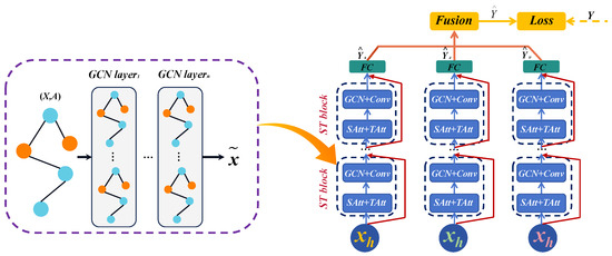
Figure 7.
Structure of ASTGCN.
Let x be a signal on graph G and Ψ be the eigenvector matrix of the Laplace matrix of graph G. The graph Fourier transform (GFT) (denoted as TGFT) and the inverse graph Fourier transform (IGFT) [32] (denoted as TIGFT) of x are defined as:
Based on the above definition, the convolution operation in graph signal processing can be defined as follows:
The above equation is further obtained by simplification:
Let Hx1 represent the right middle bracket part in the above equation; then, it is obvious that Hx1 is a graph shift operator, whose frequency response is the spectrum of x1. Equation (10) is essentially the basis for the study of graph convolution, on which different graph convolution operators can be obtained by different settings of the learnable parameters of Hx1. In this paper, we introduce a graph convolution method based on the fixation of Hx1, which is defined as follows:
where σ is the activation function; A is the adjacency matrix of the added self-loop; D is the degree matrix; and W is the learnable weight matrix. According to the principle of Equation (11), a graph convolutional layer can be constructed, and a graph convolutional neural network model can be obtained by stacking multiple layers of graph convolutional layers.
To achieve cluster-level power forecasting, assume that a power sequence is recorded at each node in cluster G. We use to denote all feature values of node i at time t, to denote all feature values of all nodes at time t, and to denote all feature values of all nodes over the entire time period τ. Additionally, we define as the power of node i at a future time t.
4.2. Photovoltaic Cluster Power Short-Term Interval Prediction Framework
As illustrated in Figure 8, the proposed ultra-short-term interval forecasting framework for PV-cluster power under multi-spatio-temporal scales is implemented in two sequential stages: cluster partitioning and interval generation. First, K-Modes clustering is employed to group the plants: cloud cover, irradiance, temperature, wind-speed NWP variables, historical PV power, and the geographical coordinates of each plant are fed into the algorithm with the preset cluster number K = 3, so that stations sharing similar meteorological, electrical, and locational signatures are merged into one sub-cluster. Next, the ASTGCN model is independently trained on each sub-cluster to deliver point forecasts of sub-cluster power; the cluster-wide ultra-short-term deterministic forecast is then obtained by summing the three individual outputs. To move from point to interval forecasts, the error distribution at every predicted time stamp is modeled via kernel-density estimation (KDE) [33]. Since the choice of kernel has negligible influence on non-parametric accuracy, the Gaussian kernel is uniformly adopted. Finally, combining the deterministic forecasts with the estimated error densities yields the cluster-level ultra-short-term power prediction intervals. To demonstrate the superiority of the proposed architecture, Table 1 summarizes the hyperparameters and execution times of the proposed model and the benchmark approaches.
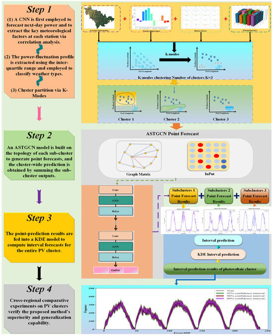
Figure 8.
Photovoltaic cluster power short-term interval forecasting framework diagram.

Table 1.
Operating parameters and runtime data for each model.
4.3. Performance Evaluation Metrics for Interval Prediction
To provide a more intuitive and accurate characterization of the proposed method for photovoltaic power interval forecasting and to facilitate the development of a model better suited to cluster-wise interval prediction, this paper computes evaluation metrics based on the obtained prediction intervals. Equation (12) defines the reliability metric—Prediction Interval Coverage Probability (PICP); Equation (14) defines the sharpness metric—Prediction Interval Normalized Average Width (PINAW); and Equation (16) introduces a composite metric—the Coverage Width-based Criterion (CWC)—that simultaneously assesses both reliability and sharpness.
In the above, is a Boolean variable; and denote the upper and lower bounds at time i, respectively. PINAW is normalized by the range R of the actual values, which enhances the comparability of prediction-interval widths across different datasets. After selecting an appropriate interval-forecasting model, the probability that the true PV power value falls inside the prediction interval should be close or identical to the pre-assigned confidence level 1 − α. Hence, the model’s reliability metric defined as the deviation between the empirical coverage PICP and the nominal confidence, 1 − α is calculated as follows:
A higher PICP indicates that the prediction interval covers the actual observations more adequately, whereas a smaller PINAW signifies a narrower and thus more precise interval.
By comparing the CWC index, one can judge whether the prediction interval achieves the narrowest possible width while satisfying the prescribed coverage. According to (15)–(17), the deviation between PICP and the nominal confidence level μ is amplified through the parameter η; the smaller η is, the lighter the penalty when PICP falls short of μ. If PICP exactly reaches μ, CWC collapses to PINAW.
The key advantage of the categorical metric is that it simultaneously accounts for both coverage and width, thereby providing an overall indication of a model’s reliability and sharpness; nevertheless, it cannot, on its own, dissect the individual effects on coverage and bandwidth. Consequently, when evaluating PV power interval forecasts, the categorical metric can serve as a comprehensive assessment, but explicit reference to coverage and width remains indispensable for a clear appraisal of model reliability and validity.
5. Case Study
To evaluate the proposed spatio-temporal K-Modes clustering, ASTGCN point forecasting, and KDE interval forecasting, 20 PV plants in Jilin Province (615 MW total) are used. Power is sampled every 15 min; only 05:00–17:00 data are retained, with nighttime values set to zero. Records exceeding capacity or negative are removed, gaps are cubic-spline interpolated, and each plant’s power is Min–Max normalized. The dataset spans 1 January 2017–31 December 2018, containing plant locations, power, and NWP variables (cloud cover, irradiance, temperature, wind speed). The first eleven months of 2018 serve for training and the last month for testing; the forecast horizon is 24 h (96 points).
5.1. Overall Evaluation of the Model
Table 2 lists the installed capacity and geographic coordinates of the 20 PV plants and, by means of the complex-fluctuation weather extraction method, gives the annual count of such days for each site. Spatial correlation stems from plant locations: different coordinates lead to different simultaneous outputs. Temporal correlation is captured by the number of complex-fluctuation days, which reflects the intra-day variability of power; this count varies markedly across plants over a year.
Table 2.
Photovoltaic cluster-related information.
When clustering with K-Modes, the choice of K directly affects forecast accuracy. If K is smaller than the true number of similarity groups, plants with distinct characteristics are forced into the same cluster; conversely, if K is larger, similar plants are split. Table 3 quantifies this impact on interval prediction quality: for K = 3, the cluster-averaged interval achieves the highest coverage while maintaining the narrowest bandwidth.
Table 3.
Effect of different numbers of clusters on interval prediction accuracy at 90% confidence interval.
Figure 9 shows the spatial distribution of 20 PV cluster power plants in Jilin province and the clustering results of PV power plants after using K-Modes clustering. From Figure 9, it can be seen that the power output of each PV plant differs at the same point in time, which is caused by the different spatial geographic distribution of each PV plant. And after using K-Modes clustering, sub-cluster 2 only has power plants 1, 3, and 6, sub-cluster 3 only has power plants 4, 9, and 13, and the rest of the power plants belong to cluster 1. This indicates that the other meteorological characteristics of power plants with similar spatial geographic locations in a certain region are not necessarily similar, which is caused by the different internal structures of different PV power plants. Therefore, the classification of PV clusters cannot be based on spatial characteristics alone.
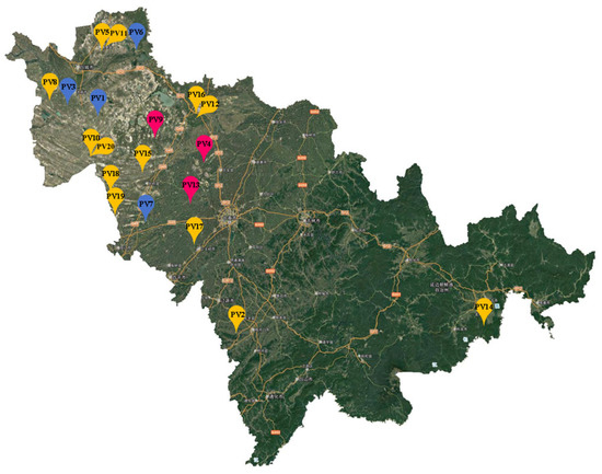
Figure 9.
Clusters of PV plants based on K-Modes clustering. (The Chinese character “吉林市”, meaning “Jilin City”, all other labels are as described in the main text).
After partitioning the PV cluster, the ASTGCN model is used to forecast each sub-cluster individually, and the final cluster-wide prediction is obtained by summation. To validate the superiority of the proposed approach, it is compared with traditional machine-learning and deep-learning baselines under the following error metrics. As shown in Figure 10, panels (a)–(f) display the prediction curves of the benchmark models, while panel (g) presents the proposed ASTGCN model, whose predicted curve closely tracks the actual values with the highest accuracy, thereby demonstrating the effectiveness of the proposed method.
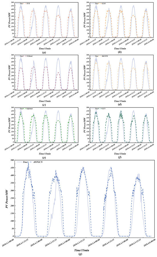
Figure 10.
Photovoltaic cluster point prediction results. (a) SVR; (b) ELM; (c) XGBoost; (d) BiLSTM; (e) Informer; (f) GCN; (g) ASTGCN. Each subfigure compares the predicted and actual power output over the forecast horizon.
To quantify the final forecasting results of each model, this paper employs four evaluation metrics: Root Mean Square Error (RMSE) [34], Mean Absolute Percentage Error (MAPE) [35], Mean Absolute Error (MAE) [36], and the coefficient of determination (R2) [37]. RMSE and MAE are scale-independent, while R2 indicates the proportion of variance in the observed values explained by the predictions. Generally, lower RMSE, MAE, and MAPE values together with a higher R2 signify superior predictive performance; the exact formulas are given in Abbreviations, Appendix A. Definition of Error Metrics. The bar chart comparing the prediction errors of all models is presented in Figure 11.
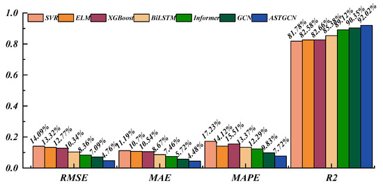
Figure 11.
Comparison of error metrics of different models.
In accordance with the “Technical Requirements for Power Forecasting of Photovoltaic Power Stations,” this paper investigates prediction intervals for the PV cluster at confidence levels of 95%, 90% and 80%; Figure 12 displays the cluster-wide forecasts generated by the proposed method under these three levels, and Table 4 quantifies the corresponding evaluation metrics. At the 95% level, the upper bound is highest and the lower bound is lowest, so the greatest number of observed power points falls inside the interval, the coverage probability reaches 95.14%, and the bandwidth is also the widest at 24.44%, indicating the strongest ability to cover the true values and the highest reliability. When the confidence level is reduced to 90% the bounds tighten, a small fraction of observations is excluded, and both coverage and bandwidth decrease; likewise, the 80% level narrows the band still further. According to Table 4, the 95% interval is the most reliable, yielding the smallest RACE of 0.14% (1.94% and 2.36% lower in absolute terms than those at 90% and 80%, respectively), while conversely the 80% interval is the sharpest, with the minimum PINAW of 15.99% and the highest composite skill score CWC, demonstrating that it achieves the most compact representation of uncertainty while tolerating only a slight loss in coverage. Figure 13 presents the error probability histogram. The fitted density curve is smooth and closely matches the empirical distribution, indicating accurate residual density estimation and providing a reliable basis for confidence quantification. Overall, the proposed method satisfies the general principles of interval forecasting and delivers satisfactory performance across all three confidence levels.
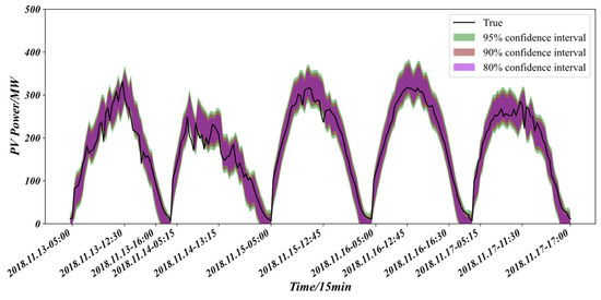
Figure 12.
Prediction of PV clusters based on K-Modes clustering and KDE model with different confidence intervals.
Table 4.
Evaluation indicators of PV cluster prediction with different confidence intervals for the proposed method in this paper.
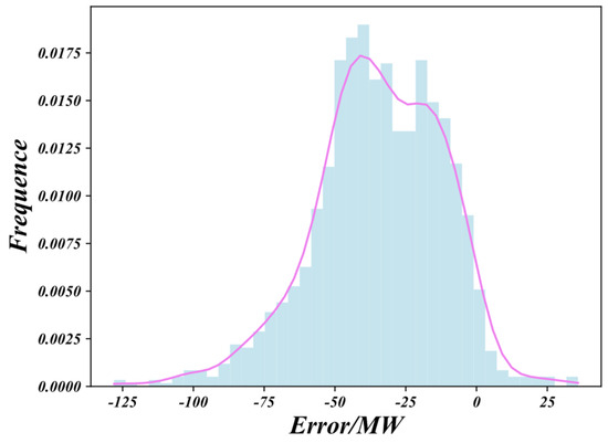
Figure 13.
Probability density histogram (MW) of the proposed method in this paper. (All negative signs are shown as short hyphens ‘-’, which are equivalent to the mathematical minus sign ‘−’).
5.2. Validity Verification Considering Spatio-Temporal Properties
This paper incorporates both temporal and spatial characteristics when clustering photovoltaic (PV) stations. Temporal features (the annual number of fluctuating days for each plant) and spatial features (geographical coordinates) are fed into the clustering algorithm. To validate this idea, the resulting interval forecasts are compared with those produced by three alternative strategies: Method 1 uses K-Modes driven solely by spatial attributes; Method 2 uses K-Modes driven solely by temporal attributes; and Method 3 applies K-Modes without considering either spatial or temporal information.
Figure 14 and Table 5 jointly present the interval-forecast curves and evaluation metrics produced by K-Modes clustering when temporal and/or spatial attributes are selectively injected. Compared with the three ablated alternatives, the proposed spatio-temporal strategy simultaneously achieves the highest coverage and the narrowest bandwidth: coverage rises by 0.84% and bandwidth falls by 4.81% relative to the space-only variant, and the gains are even larger (+4.01% coverage and −7.20% bandwidth) against the time-only variant. Relying on a single dimension—either the annual fluctuation-day histogram or the GPS coordinates—yields overly conservative envelopes because the resultant centroids fail to isolate homogenous regimes: spatial-only grouping ignores cloud-advection-driven ramping signatures, while temporal-only grouping disregards longitude–latitude phase shifts, leaving substantial intra-cluster heterogeneity that must be absorbed by wider intervals. Consequently, both single-feature schemes are forced to sacrifice sharpness to maintain nominal coverage. The “neither-time-nor-space” baseline performs worst: during steep downward ramps, the interval cannot follow the drop, exposing up to 11% of true values and yielding the lowest PICP (89.15%), a clear sign that the absence of guiding features erodes the model’s ability to recognize fluctuation patterns. In contrast, the simultaneous inclusion of fluctuation-day counts and geo-coordinates forces K-Modes to form centroids in a hybrid temporal–spatial metric space, producing clusters whose members share both similar meteorological statistics and correlated irradiance paths; the resulting residuals are nearly homoscedastic and approximately Gaussian, allowing KDE to adopt a smaller kernel width while still capturing the true error mass. Hence, the proposed spatio-temporal clustering not only captures power ramps more accurately and raises coverage but also delivers the thinnest prediction band, achieving the desirable “high coverage–low bandwidth” outcome without trading away reliability.
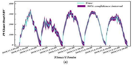
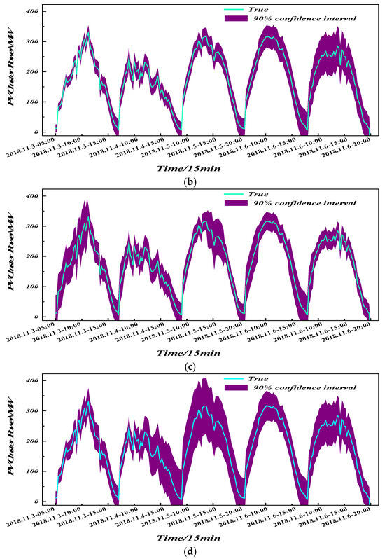
Figure 14.
Prediction effect of clustering with different inputs at 90% confidence interval. (a) Clustering prediction considering spatio-temporal characteristics. (b) Clustering prediction considering only temporal characteristics. (c) Clustering prediction considering only spatial characteristics. (d) Clustering prediction without considering spatio-temporal characteristics.
Table 5.
Evaluation index of clustering prediction with different inputs at 90% confidence interval.
5.3. Validation of K-Modes Cluster Partitioning
After cluster partitioning, PV plants within a sub-cluster usually share similar meteorological characteristics and analogous generation processes; this homogeneity not only smooths the forecasting errors of the sub-cluster but also provides approximately identically distributed residual samples for subsequent kernel density estimation, thereby simultaneously improving the reliability and sharpness of the interval forecasts. To verify the effectiveness of the K-Modes partitioning method adopted in this paper, two comparative experiments are designed: the first performs interval prediction after K-Means clustering, and the second conducts interval prediction directly on the entire cluster without any partitioning. As shown in Figure 15, the K-Means-based interval prediction performs well, offering a large upper bound that almost encloses all actual power observations; however, this also increases the bandwidth. Although most points in the high-power segment are covered, the significantly elevated upper bound causes overall bandwidth inflation, reflecting that the continuous distance metric forcibly merges stations with similar amplitudes but different fluctuation phases, resulting in a multimodal and heavy-tailed residual distribution that compels KDE to widen the kernel width to maintain coverage; consequently, K-Means clustering works better in high-power periods but slightly worse in low-power periods. When no clustering is applied and interval prediction is carried out on the entire cluster, the capture of fluctuations is less pronounced; although a certain interval coverage is satisfied, the bandwidth is also increased. In contrast, the proposed method reduces the bandwidth of the power interval while maintaining a reasonable distribution of the upper and lower bounds, allowing more actual power points to fall within the interval; therefore, it is more accurate and reasonable than traditional methods and enables KDE to capture the same probability mass within a narrower bandwidth.
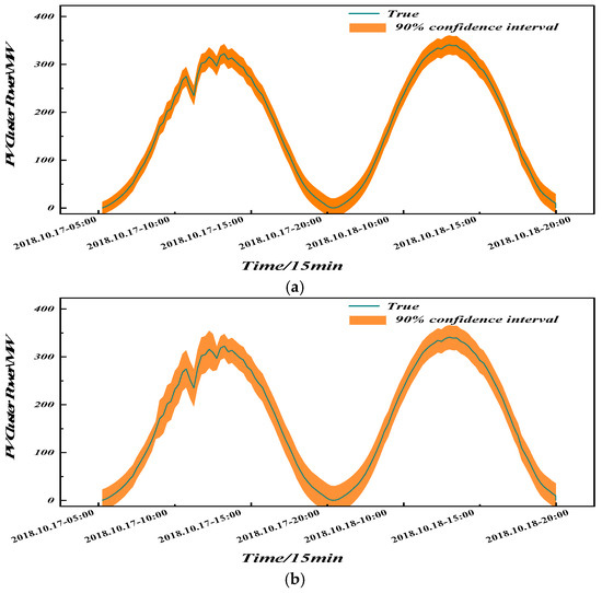
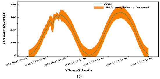
Figure 15.
The effect of different clustering methods at 90% confidence interval. (a) confidence interval. (b) The effect of using K-Means clustering at 90% confidence interval. (c) Effect of no clustering at 90% confidence interval.
The interval prediction evaluation metrics using K-Modes clustering, K-Means clustering and a single cluster with different confidence intervals are given in Table 6. The comparison with the K-Modes clustering evaluation metrics further proves the above statement that the proposed method in this paper has the highest score in both reliability and acuity, as well as skill. At three confidence intervals of 95%, 90%, and 80%, the interval coverage of K-Means clustering is 0.97%, 2.29% and 0.56% lower than that of this paper’s method, while the bandwidth increases by 2.9%, 2.67% and 2.28%, respectively, than that of this paper’s method. The results of interval prediction without clustering are the least effective among the three algorithms, and the interval prediction accuracy is the lowest. This also proves the necessity of clustering the PV plants in the interval prediction of PV clusters.
Table 6.
Evaluation indicators of PV cluster prediction with different confidence intervals for different clustering methods.
5.4. Experiments on PV Clusters in Other Regions
To verify the generalizability of the proposed approach, a full-year experiment was conducted using measured data from a 194 MW PV cluster in Hebei Province from 15 August 2018 to 15 August 2019, split 8:2 for training and testing. The cluster comprises ten plants, each providing 15 min PV output and corresponding NWP variables; benchmark models remain identical to the main text. Prediction intervals at 95%, 90% and 80% confidence levels were produced with the proposed method; forecasts under the three levels are shown in Figure 16, and metrics are listed in Table 7. Although Hebei exhibits faster cloud advection, gentler terrain and consequently higher-frequency irradiance fluctuations, together with alternating summer thunderstorms and winter haze events that raise meteorological complexity above the original Jilin scenario, Table 7 confirms that the method retains statistical consistency—PICP reaches 92.76% with RACE only 0.27% at 95%, while PINAW monotonically narrows from 29.17% to 18.31% and CWC drops to 0.21 as confidence decreases—thereby demonstrating the approach’s cross-regional generalizability.
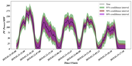
Figure 16.
Forecasts under different confidence levels in the additional scenario using the proposed method.
Table 7.
Evaluation metrics of the PV-cluster prediction under different confidence levels in the additional scenario using the proposed method.
6. Conclusions and Outlook
6.1. Conclusions
Interval forecasts for PV clusters provide grid operators with richer information than point forecasts. By integrating the spatial and temporal characteristics of each plant, the proposed framework enriches feature representation and applies K-Modes clustering—using geographical, meteorological, and power-coupling features—to group similar stations into homogeneous sub-clusters. Each sub-cluster is modeled using an ASTGCN to capture both static and dynamic spatial dependencies, and the aggregated outputs provide cluster-wide point predictions. Kernel density estimation (KDE) is then applied to the residuals to generate probabilistic prediction intervals. Experimental results show that the proposed method consistently outperforms alternative clustering strategies across multiple confidence levels. At the 90% confidence level, PICP improves by 4.01% and PINAW decreases by 7.20%. Compared with other clustering methods, K-Modes increases coverage by 0.97–2.29% while reducing average bandwidth. Cross-regional tests further validate the generalizability of the approach.
6.2. Outlook
Although the proposed framework integrates K-Modes clustering, ASTGCN-based point forecasting, and KDE-based interval estimation effectively, several limitations remain. The adjacency matrix in ASTGCN is static, combining meteorological correlation and geographical distance, which limits its ability to reflect time-varying spatial dependencies under seasonal or extreme weather conditions. Additionally, discretizing continuous meteorological variables for K-Modes introduces truncation errors, potentially leading to misclassification of boundary stations—especially in complex terrain—and slightly degrading interval coverage. Future work will focus on developing dynamic graph learning mechanisms, such as time-adaptive or sliding-window-based adjacency updates, to better capture evolving spatial relationships. Moreover, embedding high-dimensional meteorological data into a latent space before clustering will be explored to reduce discretization error and improve clustering accuracy. These improvements will enhance the robustness and scalability of the forecasting framework, supporting the integration of large-scale photovoltaic systems under the “dual carbon” goals.
Author Contributions
Conceptualization, Z.W. (Zhong Wang) and M.Y.; methodology, Z.W. (Zhong Wang).; software, Z.W. (Zhong Wang); validation, M.Y., Z.W. (Zhong Wang), and Y.L.; formal analysis, Z.W. (Zhao Wang) and B.W.; investigation, Z.W. (Zhao Wang) and Z.W. (Zheng Wang); resources, Y.L.; data curation, Z.W. (Zhao Wang); writing—original draft, Z.W. (Zhao Wang); writing—review and editing, M.Y.; visualization, Y.L. and Z.W. (Zhao Wang); supervision, M.Y.; project administration, Z.W. (Zheng Wang) and B.W.; funding acquisition, Y.L. All authors have read and agreed to the published version of the manuscript.
Funding
This research received no external funding.
Data Availability Statement
The datasets presented in this article are unavailable due to privacy restrictions.
Conflicts of Interest
Authors Bo Wang, Zhao Wang, and Zheng Wang were employed by the company State Grid Corporation of China; Yitao Li was employed by the company Huaneng Group of China. The remaining authors declare that the research was conducted in the absence of any commercial or financial relationships that could be construed as a potential conflict of interest.
Abbreviations
The following abbreviations are used in this manuscript:
| PV | Photovoltaic |
| NWP | Numerical Weather Prediction |
| ASTGCN | Attention-based spatiotemporal graph convolutional network |
| DGECN | Deep Attentional Embedded Graph Clustering |
| CNN | Convolution Neural Network |
| BiLstm | Bidirectional LSTM |
| Xgboost | Extreme gradient boosting |
| GCN | Gradient Boosting Regression |
| ELM | Extreme Learning Machine |
| Informer | Residual Attention Transformer |
| SVR | Support Vector Regression |
| RMSE | Root Mean Square Error |
| MAE | Mean Absolute Error |
| MAPE | Mean Absolute Percentage Error |
| R2 | R square |
| IMF | Intrinsic Mode Function |
| Tem | Temperature |
| Cloud | Cloud |
| SHF | Sensible heat flux |
| LHF | Latent heat flux |
| Srad | Shortwave radiation |
| Lrad | Longwave radiation |
| Hum | Humidity |
| LP | Large precipitation |
| CP | Convective precipitation |
| MF | Momentum flux |
| 170_ws | 170 m wind speed |
| 100_ws | 100 m wind speed |
| SAtt | Spatial Atten-tion |
| TAtt | Temporal Attention |
| GCN | Graph Convolution |
| Conv | Convolution |
| FC | Fully connected |
| ST block | Spatial-Temporal block |
| PICP | PI coverage probability |
| PINAW | PI normalized averaged width |
| CWC | coverage width-based criterion |
Appendix A
Definition of Error Metrics
where n is the total number of samples, the actual power at time i is expressed as , the predicted power at time i is , the normalized value at time i is , is the power-on capacity at time i.
References
- Wang, H.; Lu, Z.; Wojtasiak, A.; Owyong, S.; Sun, B.; Fang, Y.; Vassigh, S.; Lin, A. Biomimetic self-shading walls via 3D-printing for reduced heat gain: Multiscale learning using graph neural networks to predict solar radiation absorption. Build. Environ. 2025, 279, 113048. [Google Scholar] [CrossRef]
- Liu, Y.; Wang, Y.; Xu, P.; Xue, Y.; Chen, Y.; Zhang, D. BuildSTG: A multi-building energy load forecasting method using spatio-temporal graph neural network. Energy Build. 2025, 347, 116190. [Google Scholar] [CrossRef]
- Tan, S.; Xie, P.; Vasquez, J.C.; Guerrero, J.M. Developments, challenges and future opportunities in cybersecure microgrid control. Nat. Rev. Electr. Eng. 2025, 2, 522–540. [Google Scholar] [CrossRef]
- Wu, Z.; Pan, S.; Chen, F.; Long, G.; Zhang, C.; Yu, P.S. A Comprehensive Survey on Graph Neural Networks. IEEE Trans. Neural Netw. Learn. Syst. 2021, 32, 4–24. [Google Scholar] [CrossRef]
- Yang, M.; Jiang, Y.; Xu, C.; Wang, B.; Wang, Z.; Su, X. Day-ahead wind farm cluster power prediction based on trend categorization and spatial information integration model. Appl. Energy 2025, 388, 125580. [Google Scholar] [CrossRef]
- Bai, M.; Zhou, G.; Yao, P.; Dong, F.; Chen, Y.; Zhou, Z.; Yang, X.; Liu, J.; Yu, D. Deep multi-attribute spatial–temporal graph convolutional recurrent neural network-based multivariable spatial–temporal information fusion for short-term probabilistic forecast of multi-site photovoltaic power. Expert Syst. Appl. 2025, 279, 127458. [Google Scholar] [CrossRef]
- Yang, Y.; Liu, Y.; Zhang, Y.; Shu, S.; Zheng, J. DEST-GNN: A double-explored spatio-temporal graph neural network for multi-site intra-hour PV power forecasting. Appl. Energy 2025, 378, 124744. [Google Scholar] [CrossRef]
- Ye, J.; Li, J.; Su, R.; Yang, S.; Huang, Y.; Zhao, C. DFGCN: Decoupled dual-flow dynamic graph convolutional network for multivariate time series forecasting. Knowl.-Based Syst. 2025, 323, 113720. [Google Scholar] [CrossRef]
- Sun, F.; Li, L.; Bian, D.; Ji, H.; Li, N.; Wang, S. Short-term PV power data prediction based on improved FCM with WTEEMD and adaptive weather weights. J. Build. Eng. 2024, 90, 109408. [Google Scholar] [CrossRef]
- Zhao, H.; Huang, X.; Xiao, Z.; Shi, H.; Li, C.; Tai, Y. Week-ahead hourly solar irradiation forecasting method based on ICEEMDAN and TimesNet networks. Renew. Energy 2024, 220, 119706. [Google Scholar] [CrossRef]
- Yang, M.; Che, R.; Yu, X.; Su, X. Dual NWP wind speed correction based on trend fusion and fluctuation clustering and its application in short-term wind power prediction. Energy 2024, 302, 131802. [Google Scholar] [CrossRef]
- Guo, M.; Kou, P.; Tian, R.; Zhang, Y.; Liang, D. Speed Probabilistic Forecasting of Multiple Wind Turbines in a Wind Farm Based on Bayesian Graph Convolutional Neural Network. Trans. China Electrotech. Soc. 2025, 40, 5539–5552. [Google Scholar]
- Yang, M.; Shen, X.; Huang, D.; Su, X. Fluctuation Classification and Feature Factor Extraction to Forecast Very Short-Term Photovoltaic Output Powers. CSEE J. Power Energy Syst. 2025, 11, 661–670. [Google Scholar]
- Yin, L.; Zhou, H. Multiscale convolutional attention Transformer based on transfer learning for temperature forecasting of ultra-supercritical coal-fired power plant reheater. Appl. Soft Comput. 2025, 186, 114068. [Google Scholar] [CrossRef]
- Liu, C.-L.; Lu, S.-R.; Chen, Y.-T.; Lee, C.-H. Temporal attention for photovoltaic power forecasting using all-sky imagery. Sustain. Energy Grids Netw. 2025, 44, 101985. [Google Scholar] [CrossRef]
- Yang, M.; Huang, Y.; Wang, Z.; Wang, B.; Su, X. A Framework of Day-Ahead Wind Supply Power Forecasting by Risk Scenario Perception. IEEE Trans. Sustain. Energy 2025, 16, 1659–1672. [Google Scholar] [CrossRef]
- Hasnat, A.; Asadi, S.; Alemazkoor, N. A graph attention network framework for generalized-horizon multi-plant solar power generation forecasting using heterogeneous data. Renew. Energy 2025, 243, 122520. [Google Scholar] [CrossRef]
- Tan, S.; Xie, P.; Guan, Y.; Vasquez, J.C.; Guerrero, J.M.; Zhang, X. (Eds.) A Resilient Control Framework for Enhancing Cyber-Security in Microgrids. In Energy Informatics; Springer: Berlin/Heidelberg, Germany, 2025. [Google Scholar]
- Su, Z.; Wang, Y.; Wang, F.; Lin, Y.; Cui, D.; Chang, X.; Zhen, Z. Feature representation optimization and dynamic hierarchical correlation modeling based ultra-short-term probabilistic power forecasting for distributed PV. Energy Build. 2025, 347, 116308. [Google Scholar] [CrossRef]
- Sima, Q.; Zhang, X.; Yang, S.; Shen, L.; Bao, Y. Multi-scale fused Graph Convolutional Network for multi-site photovoltaic power forecasting. Energy Convers. Manag. 2025, 333, 119773. [Google Scholar] [CrossRef]
- Qiao, Y.; Zhao, P.; Wang, J.; Hu, R.; Li, M.; Yuan, X.; Li, M.; Wei, Z.; Feng, C. Multivariate Time Series forecasting based on temporal decomposition and graph neural network. Eng. Appl. Artif. Intell. 2025, 161, 112074. [Google Scholar] [CrossRef]
- Zhang, M.; Zhen, Z.; Liu, N.; Zhao, H.; Sun, Y.; Feng, C.; Wang, F. Optimal Graph Structure Based Short-Term Solar PV Power Forecasting Method Considering Surrounding Spatio-Temporal Correlations. IEEE Trans. Ind. Appl. 2023, 59, 345–357. [Google Scholar] [CrossRef]
- Zhen, Z.; Yang, Y.; Wang, F.; Yu, N.; Huang, G.; Chang, X.; Li, G. PV power forecasting method using a dynamic spatio-temporal attention graph convolutional network with error correction. Sol. Energy 2025, 300, 113770. [Google Scholar] [CrossRef]
- Qu, Z.; Hou, X.; Huang, S.; Li, D.; He, Y.; Meng, Y. Probabilistic power forecasting for wind farm clusters using Moran-Graph network with posterior feedback attention mechanism. Energy 2025, 328, 136558. [Google Scholar] [CrossRef]
- Zhao, Y.; Zhu, F.; Guan, J.; He, X.; Li, S. Radial search-based graph clustering method. Neurocomputing 2025, 655, 131421. [Google Scholar] [CrossRef]
- Shringi, S.; Saini, L.M.; Aggarwal, S.K. A review of data-driven deep learning models for solar and wind energy forecasting. Renew. Energy Focus 2025, 55, 100739. [Google Scholar] [CrossRef]
- Ma, N.; Zhao, P.; Xu, W.; Liu, A.; Zhu, H.; Shi, Z.; Wang, J. A multi-level isobaric hydrogen-electric coupled energy storage system with a wide-range operational strategy: Enhancing efficiency and flexibility in renewable-dominated power grid. Appl. Energy 2025, 401, 126783. [Google Scholar] [CrossRef]
- Kathole, A.B.; Jadhav, D.; Vhatkar, K.N.; Amol, S.; Gandhewar, N. Solar energy prediction in IoT system based optimized complex-valued spatio-temporal graph convolutional neural network. Knowl.-Based Syst. 2024, 304, 112400. [Google Scholar] [CrossRef]
- Ouyang, J.; Chu, L.; Chen, X.; Zhao, Y.; Zhu, X.; Liu, T. A K-means cluster division of regional photovoltaic power stations considering the consistency of photovoltaic output. Sustain. Energy Grids Netw. 2024, 40, 101573. [Google Scholar] [CrossRef]
- Ye, X.; Zhu, Y.; Zhang, S.; Deng, H.; Yu, P. Non-interactive K-mode clustering of high-dimensional categorical data under local differential privacy. Inf. Sci. 2025, 718, 122417. [Google Scholar] [CrossRef]
- Ma, N.; Zhao, P.; Liu, A.; Xu, W.; Wang, J. Thermodynamic analysis of natural gas/hydrogen-fueled compressed air energy storage system. Int. J. Hydrogen Energy 2024, 68, 227–243. [Google Scholar] [CrossRef]
- Siriwardana, A.N.; Kume, A. Introducing the spectral characteristics index: A novel method for clustering solar radiation fluctuations from a plant-ecophysiological perspective. Ecol. Inform. 2025, 85, 102940. [Google Scholar] [CrossRef]
- Zhou, J.; Zhou, L.; Zhao, Y.; Wu, K. Significant wave height prediction based on improved fuzzy C-means clustering and bivariate kernel density estimation. Renew. Energy 2025, 245, 122787. [Google Scholar] [CrossRef]
- Yang, M.; Jiang, Y.; Guo, Y.; Su, X.; Li, Y.; Huang, T. Ultra-short-term prediction of photovoltaic cluster power based on spatiotemporal convergence effect and spatiotemporal dynamic graph attention network. Renew. Energy 2025, 255, 123843. [Google Scholar] [CrossRef]
- Wang, P.; Feng, L.; Zhu, Y.; Wu, H. Hybrid spatial–temporal graph neural network for traffic forecasting. Inf. Fusion 2025, 118, 102978. [Google Scholar] [CrossRef]
- Wang, Y.; Zhao, X.; Li, Z.; Zhu, W.; Gui, R. A novel hybrid model for multi-step-ahead forecasting of wind speed based on univariate data feature enhancement. Energy 2024, 312, 133515. [Google Scholar] [CrossRef]
- Yang, Y.; Fan, S.; Liu, Z.; Yu, Z. WD-SGformer: High-precision wind power forecasting via dual-attention dynamic spatio-temporal learning. Energy 2025, 337, 138538. [Google Scholar] [CrossRef]


Disclaimer/Publisher’s Note: The statements, opinions and data contained in all publications are solely those of the individual author(s) and contributor(s) and not of MDPI and/or the editor(s). MDPI and/or the editor(s) disclaim responsibility for any injury to people or property resulting from any ideas, methods, instructions or products referred to in the content. |
© 2025 by the authors. Licensee MDPI, Basel, Switzerland. This article is an open access article distributed under the terms and conditions of the Creative Commons Attribution (CC BY) license (https://creativecommons.org/licenses/by/4.0/).