Abstract
Aiming at the problems that the random probability characteristics of large-scale source and load resources lead to the ineffectiveness of deterministic planning methods, the standard grid structure is difficult to adapt to the demands of diversified scenarios. This paper proposes a grid-based scenario delineation method for distribution networks based on fuzzy comprehensive evaluation and SNN-DPC (density peak clustering based on shared-nearest-neighbors). First, analyze the response characteristics of various types of flexible resources, and establish a multi-dimensional comprehensive assessment index system that integrates operational characteristics and structural features. Second, the comprehensive weights of each index in the index layer are calculated based on the DEMATEL-ANP method and the CRITIC method, and the assessment value of the intermediate layer is calculated by the fuzzy comprehensive evaluation method. Finally, the assessment value of the intermediate layer is clustered based on the improved SNN-DPC algorithm, so as to classify the distribution grid scenarios. The results indicate that the proposed method can effectively and accurately classify distribution network scenarios.
1. Introduction
With the rapid development of the domestic economy, the load of the urban center area is gradually increasing [1]. The urban distribution network gradually reveals problems with the uneven distribution of power supply points, poor quality of power supply, and un-guaranteed economic benefits, making it difficult to control the current distribution [2]. Therefore, in the planning and construction of urban power grids, it is necessary to analyze and study the existing problems in conjunction with the actual situation, so as to promote the rational planning of the power grid [3]. Traditional distribution network planning ideas generally follow the set of processes of load forecasting, spatial distribution of loads, substation siting and capacity determination, network structure design, and customer transformer capacity determination [4]. This conventional planning approach is primarily suited for ordinary distribution network configurations and falls short of addressing the complexities associated with modern distribution systems. Therefore, decomposing the distribution network planning problem and creating an integrated solution framework, and then finding higher performance solutions for the decomposed sub-problems, is a more effective technical solution, i.e., a grid-based planning scheme [5]. The introduction of grid-based planning ideas in distribution networks is a new direction in the current research on distribution network planning.
The core of the implementation of grid planning lies in how to propose corresponding planning schemes for different forms of distribution networks, and this first requires the establishment of a comprehensive evaluation system for the characteristics of the current power grid [6]. By constructing a set of scientific and comprehensive evaluation index systems of distribution networks, it can guide the future direction of distribution network planning and can meet the construction needs at different stages [7]. Meanwhile, pointing out the deficiencies in the process of distribution network operation, laying the foundation for the evaluation of the current situation of the urban distribution network, and refining the construction [8].
Existing distribution network assessment methods are mainly divided into two kinds. One is the weighted scoring method [9], which assesses the weight of each index by expert scoring, which can reflect the assessment process more intuitively. However, it is too subjective and will have a greater impact on the overall evaluation of the distribution network. The other is the threshold determination method [10], which quantitatively evaluates the distribution network through the load factor, voltage deviation, and other indexes. However, this method has poor scenario adaptation, making it difficult to cope with new types of scenarios in the distribution network with large-scale flexible resource access. Ref. [11] selects a set of multi-dimensional indicators for distribution network resilience assessment by considering the impact of multi-energy coordination, and derives the comprehensive weights of the indicators from an optimal weighting model by combining subjective and objective factors. Ref. [12] proposes a closed-loop risk assessment method based on the fuzzy evaluation method, which establishes a closed-loop operation risk assessment index system, and calculates the corresponding weights. It uses the fuzzy comprehensive evaluation method to obtain the rank conclusion of the closed-loop operation risk; its conclusion provides the theoretical basis and technical support for safe and reliable closed-loop operation of the low-voltage distribution network. Ref. [13] proposes a distribution network reliability evaluation method that considers the reliability requirements of different user types, which takes into account the objectivity of objective weighting and the flexibility of experts in determining the weights, and it overcomes the shortcomings of the similarity of the reliability index weights. Ref. [14] proposes a grid planning method for distribution grids based on artificial intelligence technology, which determines the target grids and transition grids for planning grids according to the current grid structure, and designs the load forecasting method for distribution grids in order to improve the rationality of the division of distribution grids.
The above studies provide valuable tools for the evaluation of specific dimensions of distribution networks. However, when applied to new distribution network scenarios with a high proportion of distributed energy and random access of electric vehicles, these methods show certain limitations. This study believes that it is necessary to establish a comprehensive evaluation system that integrates multiple dimensions, such as load characteristics, power supply capacity, grid level, and carrying capacity, so as to overcome the above limitations of existing methods in dealing with new distribution network scenarios. To this end, this paper proposes the indicators that can cover the planning and construction of distribution grids with the participation of flexible resources, a fuzzy comprehensive evaluation method for distribution grids based on the DEMATEL-CRITIC method, and scene clustering based on the improved SNN-DPC algorithm. Compared to traditional K-means and DPC algorithms, this method optimizes certain parameters within the algorithm, thereby reducing sensitivity to a certain extent and making it more suitable for spatial clustering.
In Section 2, the characteristics of various types of flexible resources are analyzed, and a distribution network assessment index system based on four dimensions, namely, load characteristics, power supply capacity, network frame level, and carrying capacity, is proposed. In Section 3, the evaluation value of the middle layer is calculated based on the fuzzy comprehensive evaluation method. In Section 4, the evaluated values of the middle layer are clustered based on the improved SNN-DPC algorithm as a way to classify the distribution network scenarios. In Section 5, some grids in a certain region are selected for the arithmetic analysis to evaluate the actual situation of each grid and verify the superiority of the proposed method. Compared with traditional planning methods, the innovation of the proposed framework lies in the successful combination of fuzzy comprehensive evaluation of multi-dimensional characteristics of power grids with an improved SNN-DPC clustering algorithm suitable for complex density distributions, which provides a new and quantifiable solution to solve the adaptability and differentiation of distribution network planning under large-scale flexible resource access.
2. Comprehensive Evaluation Indicator System for Distribution Grid Planning
2.1. Supply Grid Source–Load Structure
The access to large-scale distributed flexible resources makes the distribution network gradually develop from a “passive network” to an “active network”, and the source–load structure becomes more complex [15]. In order to enable the coordinated development of flexible resources and power grids, it is necessary to rationally allocate various types of flexible resources and fully explore their operating characteristics and adjustable potential. In this paper, we analyze the flexible resource characteristics of distribution networks by taking generation-side, load-side, and storage-side resources as examples.
Distributed photovoltaic: Distributed PV is characterized by stochastic, intermittent, and fluctuating characteristics, which are affected by weather and the output power changes randomly. When the penetration rate is too high, it may cause voltage overruns, and the distributed PV grid connection relies on power electronics, weakening the stability of the system [16,17].
Electric vehicle: The charging and discharging behaviors of electric vehicles are influenced by user habits and relevant tariff policies, and their adjustable potential is large. As a mobile energy storage unit, it can participate in peak shaving and valley filling, and its individual stochasticity is strong, but its group response presents dispatchable load characteristics [18,19].
Distributed energy storage: Distributed energy storage [20,21] has the effect of shaving peaks and filling valleys. Discharging during the peak period and charging during the trough period can suppress PV fluctuations and alleviate the load peak and valley differences [22].
Demand response load: Demand-responsive loads have flexible and interruptible characteristics, and their energy consumption can be temporarily changed, such as shifting, leveling, or curtailment. It can be realized by scheduling demand-responsive loads through tariffs or incentive signals, which guide users to adjust their electricity use periods [23].
2.2. Grid Characterization Indicator System for Electricity Supply
Due to the complex structure of the current distribution network and the large number of indicators, its characteristics cannot be fully described by a single indicator. This complexity directly leads to cognitive and management difficulties. Therefore, building a complete and efficient comprehensive evaluation index system is the prerequisite for achieving accurate grid planning. When the evaluation index of the distribution network is established, on the one hand, the selection of the index must start from the whole, and the actual situation and main characteristics of the distribution network must be completely displayed as much as possible [24]. On the other hand, in order to prevent the data in the indicator system from being too large and cumbersome, resulting in the overlapping of indicator information, which may lead to problems such as imprecise assessment, it is necessary to ensure the admissibility of indicators. This paper starts from four aspects: power supply grid load characteristics, power supply capacity, grid structure, and bearing capacity, constructing a comprehensive assessment system of distribution grid characteristic indexes containing the top layer, middle layer, and indicator layer, as shown in Figure 1.
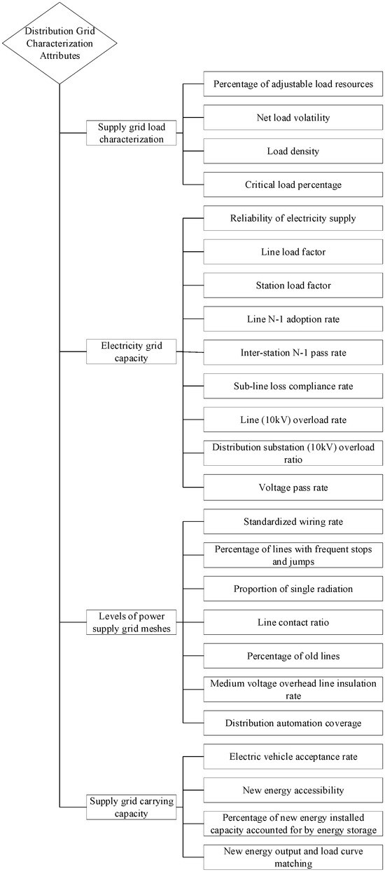
Figure 1.
Comprehensive assessment system of distribution network characterization indicators.
The middle layer indicators are an assessment of the security, equipment levels, and societal benefits that result from the participation of large-scale flexible resources in the distribution network. The indicators at the indicator level reflect the operational characteristics and weaknesses of the distribution network under the participation of flexible resources at the micro level, by portraying indicators of grid equipment, grid systems, and technology utilization. It is a direct and precise guide for distribution network planning. Most of the indicators in the indicator layer can be obtained through the data statistics, for example, the acceptance rate of electric vehicles and the amount of new energy that can be accessed can be obtained by the existing charging load, the installed capacity of new energy, and the total capacity of distribution and transformation. Part of the indicators of the calculation is more complex; the definition and calculation of this part of the indicators are as follows:
- Net load volatility
- Load density
- New energy output and load curve matching
3. Fuzzy Comprehensive Evaluation of Distribution Grid Based on DEMATEL-ANP and CRITIC Weighting Methods
3.1. Calculation of Indicator Weights for the Subjective–Objective Combination Method of Weighting
3.1.1. DEMATEL-ANP-Based Subjective Weight Calculation
Decision-Making Trial and Evaluation Laboratory (DEMATEL) is a systematic method of analyzing problems using graph theory and matrix tools to explain them. The method not only transforms interdependencies into causal groups through matrices but also discovers key factors in complex structured systems with the help of influence diagrams. And some of the indicators in the distribution grid indicators layer mentioned above interact with each other, e.g., the load peak-to-valley differential rate affects system reliability. Therefore, the Decision-Making Trial and Evaluation Laboratory method can be applied to the subjective weight calculation of the comprehensive evaluation of the distribution grid with multi-objectives and some links between indicators. The calculation process is as follows:
- 1.
- Expert scoring–constructing a direct impact matrix
First, based on the expert survey, the degree of interaction between the indicators is determined, and the degree of direct influence of indicator i on indicator j is represented by the matrix W = {ωij}, which is usually rated on a scale of 0 to 4: 0 for no direct influence, 1 for weak influence, 2 for moderate influence, 3 for strong influence, and 4 for very strong influence. The direct influence matrix is as follows:
- 2.
- Direct impact matrix normalization
Normalize the direct influence matrix. First, the elements of each row of the direct influence matrix are summed. Then, the maximum of the summation values of all rows is selected as the denominator of the regularization value. Finally, each element of the direct influence matrix is divided by the row maximum to obtain the elements of the normalized direct influence matrix. The normalized matrix is as follows:
where k is the total number of columns in the direct impact matrix; is the sum of all elements in row i of the matrix; is the maximum value of the sum of elements in all rows.
- 3.
- Integrated impact matrix construction
First, the difference between the unit matrix and the normalized direct influence matrix is computed. Then, the inverse matrix of the difference matrix is calculated. Finally, multiply the normalized direct impact matrix by the inverse matrix to obtain the combined impact matrix. The calculations are as follows:
where E is the unit matrix; A is the normalized direct impact matrix.
- 4.
- Construction of an extreme hypermatrix
Normalizing each column of the integrated influence matrix yields the weighted hypermatrix M, and then the nth power of the weighted hypermatrix is computed until the vectors of the columns of the matrix remain constant:
- 5.
- Weights solution
Each row of data in the limit hypermatrix S is the same value, and the sum of each column is 1; then any column of the limit hypermatrix can be used as the weight of each indicator. The weights of the indicators in the intermediate layer can be obtained by adding up the weights of the indicator layers, and the weights of the indicators under each intermediate layer can also be normalized to obtain the internal weights of each subsystem.
3.1.2. CRITIC Weighting Method-Based Objective Weight Calculation
The CRITIC weighting method is an objective weighting method based on data volatility. The method centers on the calculation of volatility and conflict indicators in the following steps:
- 1.
- For the n indicators of the m power supply grids, form the raw data matrix:
- 2.
- Normalize the data
Positive indicators:
Negative indicators:
- 3.
- Calculating information carrying capacity:
Volatility:
Conflictual:
Volume of information:
- 4.
- Calculation of weights
3.1.3. Composite Weighting Calculation
In order to show the authority of the experts’ experience and to make the results of the assessment more objective and reasonable, this paper adopts the geometric mean method to calculate the comprehensive weights:
where and are the subjective and objective weights of the jth distribution grid evaluation index, respectively.
3.2. Fuzzy Integrated Evaluation of Distribution Grids
3.2.1. Fuzzy Comprehensive Evaluation Set and Evaluation Matrix
In this paper, we first construct the factor set U of comprehensive evaluation, and when there are m indicators in the middle layer, , it represents a collection of data quality assessment indicators. Ranking the indicators in the middle layer, the corresponding set of evaluations is , is very good, rated 90–100, is good, rated 80–90, is ordinary, rated 60–80, and is bad, rated 0–60.
By constructing the affiliation function, the affiliation of each indicator corresponding to the evaluation set is calculated. In general, the modeling of affiliation is also different for positive-type and negative-type indicators, and the methodology for calculating affiliation is shown in Appendix A. According to the affiliation function corresponding to each indicator, the affiliation value rij of each indicator of the indicator layer corresponding to the evaluation set V is calculated separately, which in turn leads to the fuzzy evaluation matrix R.
3.2.2. Calculation of Assessed Values for Distribution Grid Indicators
Multiplying the integrated weight W of each indicator by the fuzzy evaluation matrix R, we can get the intermediate level fuzzy integrated evaluation vector H:
Finally, the vector H is multiplied by the scores of each level in the evaluation set V to obtain the final score S of the intermediate level indicator:
4. SNN-DPC-Based Grid Scenario Delineation for Distribution Networks
4.1. Cluster Center Selection Considering Shared Neighborhoods
Since the local density calculated with the truncation distance is difficult to reflect the density of the real samples, the traditional DPC algorithm deals with samples with large density differences. Therefore, this paper uses the SNN-DPC method to cluster the features of the power supply grid in the following steps:
- 1.
- Compute the shared nearest neighbor of any point i and j in the dataset:
- 2.
- Compute shared nearest neighbor similarity:
- 3.
- Calculate local density:
- 4.
- Calculate relative distance:
- 5.
- Calculate the decision value:
- 6.
- The number of clustering centers n is selected based on the number of clusters desired, and the n points with the largest are selected as centers.
- 7.
- Cluster the remaining points to the center of the cluster.
4.2. Shared Nearest Neighbor Optimization Based on Whale Optimization Algorithm
The selection of the number of shared nearest neighbors k in the SNN-DPC algorithm determines the effectiveness of the final clustering, and the value of k is currently unclear. Therefore, in this paper, the whale optimization algorithm is used to optimize the value of k by taking the minimum of the sum of the distances of all samples to the cluster center after clustering as the objective function, and the specific process is as follows:
- Set the whale population size N, the maximum number of iterations tmax, and initialize the position information.
- With the objective of minimizing the sum of distances from all points to the cluster center after clustering, the fitness of each whale is calculated, and the current optimal solution is selected.
- Updating the whale’s position based on the random probability p and the coefficient A:
When p < 0.5 and |A| < 1:
when p ≥ 0.5:
when p < 0.5 and |A| ≥ 1:
where is the current optimal solution; b is a spiral shape constant; l is a random number between −1 and 1; and is a randomly chosen whale position.
- 4.
- Perform boundary processing after the position update to ensure that the updated position is within the variable boundaries.
- 5.
- Repeat steps 2~4 until the maximum number of iterations is reached or the convergence condition is satisfied.
5. Case Study
5.1. Overview of the Algorithms
In this paper, the proposed grid-based feature clustering method for distribution networks is illustrated by taking three power supply areas in a region as examples. The load density is 8.6MW/km2. In this planning, the basis of the division of the power supply area is according to the relevant requirements of the Guiding Principles of Distribution Grid Planning. Combined with the urban master plan and control detailed planning, the three power supply areas are subdivided into some power supply grids, as shown in Figure 2. The grids selected were chosen based on stratified sampling principles to ensure the sample represents multi-type distribution networks containing high proportions of flexible resources, urban areas, suburban areas, and industrial parks.
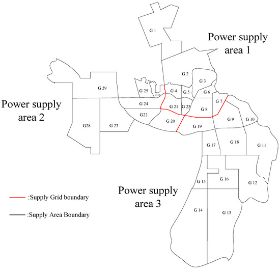
Figure 2.
Grid division of power supply in a region.
5.2. Fuzzy Integrated Evaluation Results
All simulations and algorithm implementations in this research were conducted in a Python (Version 3.11) environment. The case study data were obtained from the distribution automation system, information acquisition system, and production management system of the regional power grid. In this example, a panel of 10 experts was selected, comprising 3 from the provincial power grid company, 3 from the power design institute, and 4 from universities. The discussions among the experts were conducted anonymously and involved multiple rounds of feedback to alleviate groupthink, making the subjective evaluations of the indicators more persuasive. According to the steps of calculating the subjective and objective weights in Chapter 2, the weights of each indicator are derived as shown in Table 1, Table 2, Table 3 and Table 4.

Table 1.
Combined weights of the indicators of load characterization.
Table 2.
Combined weights of indicators of electricity supply capacity.
Table 3.
Comprehensive weights of the indicators of the grid structure.
Table 4.
Composite weights of load-bearing capacity indicators.
As shown in the table above, the composite weights of certain indicators are significantly higher than those of others. For example, the “effective connection rate” (weight 0.1749) and “standardized interconnection rate” (weight 0.2059) presented in Table 3 are the two key indicators determining the horizontal dimension of the power grid structure. Their notably higher weights compared to other indicators indicate that grid flexibility and interconnection levels are the core elements receiving the most attention from experts in the current planning process. Taking each third-level index under the grid power supply capacity as an example, according to the formula of the index affiliation function and the parameters of the index affiliation model in Appendix A, the affiliation values of each evaluation level of the grid can be obtained, as shown in Table 5.
Table 5.
Affiliation values for each evaluation level.
According to the calculation results of the integrated weights and affiliation values of the indicators, the fuzzy comprehensive evaluation vector of the grid’s power supply capacity can be derived from Equation (20):
The fuzzy comprehensive evaluation score for the grid’s power supply capacity can be derived from Equation (21), where V represents the median value of each evaluation grade within the evaluation set, :
By analogy, the rest of the middle-layer indicator scores for that grid can also be calculated by the above process, and the results of all the grid middle-layer score calculations are shown in Figure 3.
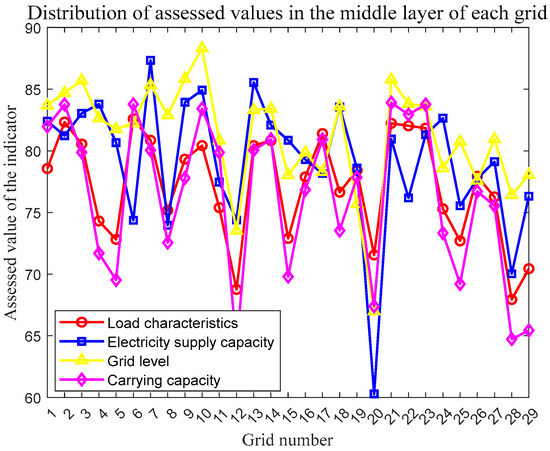
Figure 3.
Comparison of indicator scores in the middle layer of each grid.
It can be seen that most of the grids have scores of 70 or more for each indicator, evaluating them as good. And there is a correlation between the intermediate-level indicators, as evidenced by a highly consistent trend in the indicator scores. When one of the indicators performs well, the rest of the indicators are also characterized by higher scores; when one of the indicators performs slightly poorly, the rest of the indicators are also in the low-value range as a whole.
5.3. Distribution Grid Feature Clustering Results
According to the SNN-DPC clustering method proposed in Chapter 3, each grid is regarded as a point in four-dimensional coordinates, and each intermediate layer score is regarded as the coordinates of the point. Due to the correlation between the indicators, all grids can be categorized into four classes as shown in Table 6.
Table 6.
Grid categories.
Then the clustering can be performed by dividing these grids into four clusters, and according to the SNN-DPC algorithm, the local density and relative distance of each point are first calculated, and the results are shown in Figure 4.
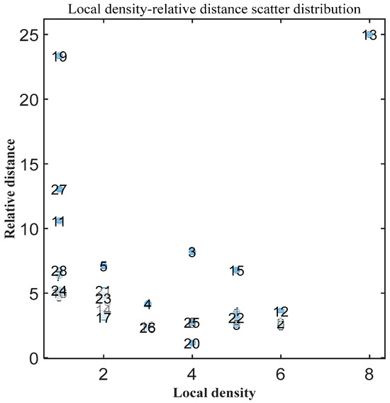
Figure 4.
Local density and weighted distance calculation results.
The numbers in the figure are the grid numbers. Based on the calculation results of local density and weighted distance, the decision value of each grid can be derived from Equation (28), and the four grids with the largest decision value are selected as the clustering centers, i.e., Grid 13, Grid 15, Grid 3, and Grid 19. Then, the rest of the grids are clustered to the clustering centers, and the position of the clustering centers is adjusted iteratively, and the final clustering results are shown in Table 7.
Table 7.
Grid clustering results.
As can be seen from Table 7, most of the grids belong to category 1, which perform well in the four indicators of the intermediate layer. The evaluation results of grids in category 2 are one level lower than those of grids in category 1. And the performance of grids in category 3 in terms of load characteristics and carrying capacity is average, which needs to be strengthened. A small number of grids belong to category 4 and perform poorly at the four indicator levels of the middle layer, so it is necessary to analyze their performance in the index layer and directly orient the investment to the weak links exposed in the evaluation.
To further validate the stability of clustering results, this case study conducted a sensitivity analysis based on subjective weighting biases. Minor adjustments were made to certain data points in the direct influence matrix—for instance, the impact weight of meeting the N-1 interconnection rate between wars on power supply reliability was reduced from 4 to 3. The final grid scenario segmentation results are as follows:
Comparing Table 7 and Table 8 reveals that the clustering results are nearly identical, with only Grid 5 being reassigned from Category 3 to Category 4. The characteristics of these adjusted grid categories are redefined in Table 9. Category 4 has also been redefined to represent distribution network scenarios characterized by poor load characteristics, moderate power supply capacity, average grid structure level, and weak load-bearing capability. This demonstrates that the distribution grid evaluation method selected in this paper exhibits strong robustness and achieves excellent clustering performance.
Table 8.
Adjusted grid clustering results.
Table 9.
Adjusted grid types.
5.4. Clustering Effectiveness Enhancement Analysis
The value of the shared nearest neighbor number k in the SNN-DPC clustering method selected for this algorithm is uncertain, so the whale optimization algorithm is used to optimize k with the objective of minimizing the sum of distances from all points in the four-dimensional coordinate system to the cluster center. The whale population size N selected for this algorithm is 10, and the maximum number of iterations tmax is 50; the iteration process is shown in Figure 5.
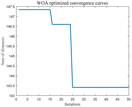
Figure 5.
Iterative process of the whale optimization algorithm.
As can be seen from Figure 5, the final result of the whale optimization algorithm for finding the optimal is 143.4096. In order to reflect the advantages of the clustering method proposed in this paper, the sum of the distances from all the points in the four-dimensional coordinate system to the center of the clustering is used as the object to compare the method proposed in this paper with the DPC algorithm and the K-means algorithm, and the results are shown in Table 10.
Table 10.
Comparison of clustering results of several algorithms.
As can be seen from Table 10, the sum of distances from all points to the clustering center in the improved SNN-DPC algorithm is smaller than that of the DPC algorithm and the K-means algorithm. Therefore, the clustering effect of the improved SNN-DPC algorithm is better, i.e., the delineated mesh scenarios and the classification of the meshes are more reasonable. In order to further highlight the superiority of the proposed method, the contour coefficients of the improved SNN-DPC algorithm and the DPC algorithm, K-means algorithm, DBSCAN, and GMM algorithm are also compared, as shown in Table 11.
Table 11.
Comparison of contour coefficients of several algorithms.
The contour coefficient reflects the effect of clustering, and the closer its value is to 1, the better the cohesion and resolution, and the last clustering effect. Table 11 shows that the clustering effect of the improved SNN-DPC algorithm is slightly better than that of other algorithms. Compared to the DPC algorithm, the contour coefficient has improved by 1%.
6. Conclusions
In this paper, we address the problem of diversification and complexity of distribution grid characteristics under the participation of large-scale flexible resources, resulting in the difficulty of adapting the conventional planning methods for distribution grids to the multifarious scenarios. It proposes a grid-based scenario delineation method for distribution grids based on fuzzy comprehensive evaluation and SNN-DPC, which is of great guiding significance for subsequent distribution grid planning. The specific contributions of this paper are the following three points:
- Starting from the four dimensions of load characteristics, power supply capacity, grid level, and carrying capacity, a complete set of distribution grid evaluation index system under the participation of large-scale flexible resources is proposed, and the attributes of the distribution network under the high proportion of flexible resource access are depicted.
- A fuzzy comprehensive evaluation model based on DEMATEL-ANP with CRITIC weighting method is developed to present the grid characteristics in the form of evaluation values.
- An improved SNN-DPC clustering algorithm based on the whale optimization algorithm is proposed; it completes the segmentation of distribution network scenarios with good results. Compared with the traditional K-means and DPC algorithms, the clustering results are more consistent with the actual grid zoning characteristics, which proves its superiority in processing the complex feature data of the distribution network.
Although this paper proposes a method for segmenting distribution network scenarios under the participation of large-scale flexible resources, its practical engineering value has not been fully demonstrated. While the scenarios outlined in this paper can guide the overall direction of grid construction, grids within the same scenario exhibit local variations, failing to adequately highlight differences between specific indicators. Future work will provide guidance on grid construction for each segment based on the identified scenarios.
Author Contributions
Conceptualization, F.Z.; Methodology, X.Y. and X.W.; Investigation, L.Z., X.Y., X.W. and F.Z.; Writing—original draft, Z.G.; Writing—review & editing, L.Z., Z.G. and H.Y. All authors have read and agreed to the published version of the manuscript.
Funding
This research was funded by the Science and Technology Project of State Grid Anhui Electric Power Co. Ltd. (Grant No. B3120924000G).
Data Availability Statement
The original contributions presented in this study are included in the article. Further inquiries can be directed to the corresponding author.
Conflicts of Interest
Authors Liuzhu Zhu, Xin Yang, Xuli Wang and Fan Zhou were employed by the State Grid Anhui Economic Research Institute. The remaining authors declare that the research was conducted in the absence of any commercial or financial relationships that could be construed as a potential conflict of interest.
Appendix A
The rule for calculating the affiliation value rij is as follows:
- Positive indicators:
- Negative indicators:
Table A1.
Indicator affiliation model and parameters.
Table A1.
Indicator affiliation model and parameters.
| Indicator | Type of Affiliation Function | Parameters of the Affiliation Function | |||
|---|---|---|---|---|---|
| a1 | a2 | a3 | a4 | ||
| Percentage of adjustable load resources | Positive | 7 | 5 | 3 | 1 |
| Net load volatility | Negative | 10 | 15 | 25 | 30 |
| Load density | Positive | 25 | 15 | 5 | 0 |
| Critical load percentage | Positive | 25 | 15 | 5 | 0 |
| Reliability of electricity supply | Positive | 100 | 99.99 | 99.98 | 99.97 |
| Line load factor | Negative | 35 | 45 | 55 | 65 |
| Station load factor | Negative | 15 | 25 | 35 | 45 |
| Line N-1 adoption rate | Positive | 100 | 90 | 70 | 50 |
| Inter-station N-1 pass rate | Positive | 85 | 70 | 50 | 35 |
| Sub-line loss compliance rate | Positive | 100 | 95 | 93 | 90 |
| Line (10 kV) overload rate | Negative | 0 | 3 | 5 | 7 |
| Distribution substation (10 kV) overload ratio | Negative | 0 | 3 | 7 | 10 |
| Voltage pass rate | Positive | 95 | 85 | 80 | 75 |
| Standardized wiring rate | Positive | 100 | 95 | 85 | 75 |
| Percentage of lines with frequent stops and jumps | Negative | 5 | 10 | 15 | 20 |
| Proportion of single radiation | Negative | 0 | 3 | 5 | 10 |
| Line contact ratio | Positive | 100 | 85 | 70 | 60 |
| Percentage of old lines | Negative | 0 | 10 | 20 | 30 |
| Medium voltage overhead line insulation rate | Positive | 100 | 95 | 93 | 90 |
| Distribution automation coverage | Positive | 100 | 85 | 70 | 60 |
| Electric vehicle acceptance rate | Positive | 35 | 25 | 15 | 5 |
| New energy accessibility | Positive | 45 | 35 | 25 | 15 |
| Percentage of new energy installed capacity accounted for by energy storage | Positive | 10 | 7 | 3 | 0 |
| New energy output and load curve matching | Positive | 50 | 40 | 30 | 20 |
References
- Tao, Y.; Zhang, J.; Guo, Z.; Xu, M.; Tan, J.; Yuan, Z. Urban Distribution Network Planning Method Considering Geographic Information based on Improved Prim Genetic Hybrid Algorithm. In Proceedings of the 2022 IEEE 5th International Conference on Automation, Electronics and Electrical Engineering (AUTEEE), Shenyang, China, 18–20 November 2022; pp. 820–824. [Google Scholar] [CrossRef]
- Jia, C.; Huang, B.; Chuai, Z.; Yan, C.; Wang, Q.; Li, H.; Zhang, S.; Chen, X. A distributed optimization method for urban active distribution networks considering SOPs and user side flexible resources based on ADMM. Syst. Sci. Control. Eng. 2024, 12. [Google Scholar] [CrossRef]
- Wang, S.C.; Sun, X.G.; Geng, J.Y.; Han, Y.; Zhang, C.Y.; Zhang, W.H. Discussion on Urban Distribution Network Planning Based on Key Tech-nologies of Smart Distribution Network. J. Phys. Conf. Ser. 2020, 1639, 012064. [Google Scholar] [CrossRef]
- Wang, C.S.; Wang, R.; Yu, H.; Song, Y.; Yu, L.; Li, P. Challenges on Coordinated Planning of Smart Distribution Networks Driven by Source-Network-Load Evolution. Proc. CSEE 2020, 40, 2385–2396. [Google Scholar] [CrossRef]
- Liu, X.O. Automatic routing of medium voltage distribution network based on load complementary characteristics and power supply unit division. Int. J. Electr. Power Energy Syst. 2021, 133, 106467. [Google Scholar] [CrossRef]
- Wu, Q.; Peng, C. Comprehensive Benefit Evaluation of the Power Distribution Network Planning Project Based on Improved IAHP and Multi-Level Extension Assessment Method. Sustainability 2016, 8, 796. [Google Scholar] [CrossRef]
- Liu, Z.W.; Xie, Q.Y.; Dai, L.; Wang, H.L.; Deng, L.; Wang, C.; Zhang, Y.; Zhou, X.X.; Yang, C.Y.; Xiang, C.; et al. Research on comprehensive evaluation method of distribution network based on AHP-entropy weighting method. Front. Energy Res. 2022, 10, 975462. [Google Scholar] [CrossRef]
- Zhang, L.Y.; Wu, G.L.; Yang, J.Y.; Jia, S.R.; Zhang, W.; Sun, W.Q. Comprehensive evaluation index system of total supply capability in distribution network. IOP Conf. Ser. Earth Environ. Sci. 2018, 108, 052065. [Google Scholar] [CrossRef]
- Hu, T.M.; Sung, S.Y.; Sun, J.; Ai, X.W.; Ng, P.A. A linear transform scheme for building weighted scoring rules. Intell. Data Anal. 2012, 16, 383–407. [Google Scholar] [CrossRef]
- Wang, L.; Verhagen, S. A new ambiguity acceptance test threshold determination method with controllable failure rate. J. Geod. 2015, 89, 361–375. [Google Scholar] [CrossRef]
- Zhao, Q.; Du, Y.; Zhang, T.; Zhang, W. Resilience index system and comprehensive assessment method for distribution network considering multi-energy coordination. Int. J. Electr. Power Energy Syst. 2021, 133, 107211. [Google Scholar] [CrossRef]
- Li, J.; Lin, S.; Li, J.; Luo, Y.; Mao, C.; Li, H.; Wang, D.; Peng, W.; Guan, Z. Risk assessment method of loop closing operation in low voltage distribution network based on fuzzy comprehensive evaluation. Energy Rep. 2023, 9 (Suppl. S3), 312–319. [Google Scholar] [CrossRef]
- Wu, J.; Zheng, J.; Mei, F.; Li, K.; Qi, X. Reliability evaluation method of distribution network considering the integration impact of distributed integrated energy system. Energy Rep. 2022, 8 (Suppl. S13), 422–432. [Google Scholar] [CrossRef]
- Fu, G.H.; Chen, D.X.; Sun, Y.; Xia, J.; Wang, F.F.; Zhu, L.H. Research on Grid Planning Method of Distribution Network Based on Artificial Intelligence Technology. In Multimedia Technology and Enhanced Learning. ICMTEL; Springer: Cham, Switzerland, 2021; Volume 387. [Google Scholar] [CrossRef]
- Su, Z.E.; Zheng, G.Q.; Wang, G.D.; Mu, Y.; Fu, J.T.; Li, P.P. Multi-objective optimal planning study of integrated regional energy system considering source-load forecasting uncertainty. Energy 2025, 319, 134861. [Google Scholar] [CrossRef]
- Wang, R.; Ji, H.; Li, P.; Hao, Y.; Zhao, J.; Zhao, L.; Zhou, Y.; Wu, J.; Bai, L.; Yan, J.; et al. Multi-resource dynamic coordinated planning of flexible distribution network. Nat. Commun. 2024, 15, 4576. [Google Scholar] [CrossRef] [PubMed]
- Yaghoubi, E.; Yaghoubi, E.; Yusupov, Z.; Maghami, M.R. A Real-Time and Online Dynamic Reconfiguration against Cyber-Attacks to Enhance Security and Cost-Efficiency in Smart Power Microgrids Using Deep Learning. Technologies 2024, 12, 197. [Google Scholar] [CrossRef]
- Zhou, M.; Wu, Z.; Li, G. Large-Scale Distributed Flexible Resources Aggregation. In Power System Flexibility; Power Systems; Springer: Singapore, 2023. [Google Scholar] [CrossRef]
- Maghami, M.R.; Thang, K.F.; Mutambara, A.G.O.; Firoozi, A.A.; Yaghoubi, E.; Jahromi, M.Z.; Yaghoubi, E. Optimized planning of electric vehicle charging infrastructure for grid performance improvement. Discov. Sustain. 2025, 6, 706. [Google Scholar] [CrossRef]
- Yang, H.; Chen, Q.; Tang, K.; Zhang, D.; Shen, Y. Flexibility aggregation and cooperative scheduling for distributed resources using a virtual battery equivalence technique. Energy 2025, 334, 137770. [Google Scholar] [CrossRef]
- Yang, H.; Chu, Y.; Ma, Y.; Zhang, D. Operation Strategy and Optimization Configuration of Hybrid Energy Storage System for Enhancing Cycle Life. J. Energy Storage 2024, 95, 112560. [Google Scholar] [CrossRef]
- Lin, Y.; Luo, H.; Chen, Y.; Yang, Q.; Zhou, J.; Chen, X. Enhancing Participation of Widespread Distributed Energy Storage Systems in Frequency Regulation Through Partitioning-Based Control. Prot. Control. Mod. Power Syst. 2025, 10, 76–89. [Google Scholar] [CrossRef]
- Zhang, Z.S.; Du, X.H.; Shang, Y.K.; Zhang, J.S.; Zhao, W.; Jia, S. Research on Demand Response Potential of Adjustable Loads in Demand Response Scenarios. Energy Eng. 2024, 121, 1577–1605. [Google Scholar] [CrossRef]
- Luo, N.; Lu, Z.Y.; Liu, J.S.; Zhang, P.C.; Chen, L.D.; He, H.Y. Research on Evaluation Index System of County Distribution Network Planning Under New Power System. In Proceedings of the 2024 the 9th International Conference on Power and Renewable Energy (ICPRE), Guangzhou, China, 20–23 September 2024; pp. 506–511. [Google Scholar] [CrossRef]


Disclaimer/Publisher’s Note: The statements, opinions and data contained in all publications are solely those of the individual author(s) and contributor(s) and not of MDPI and/or the editor(s). MDPI and/or the editor(s) disclaim responsibility for any injury to people or property resulting from any ideas, methods, instructions or products referred to in the content. |
© 2025 by the authors. Licensee MDPI, Basel, Switzerland. This article is an open access article distributed under the terms and conditions of the Creative Commons Attribution (CC BY) license (https://creativecommons.org/licenses/by/4.0/).