Abstract
Accurately quantifying the impact of weather on dynamic grid carbon intensity is crucial for power system decarbonization. This study proposes a novel, interpretable machine learning framework integrating tree-based models with SHapley Additive exPlanations (SHAP) to quantify this impact across multiple timescales via a standardized “Weather Share” metric. Applied to city-level hourly data from China, the analysis reveals that meteorological variables collectively explain 21.64% of the hourly variation in carbon intensity, with air temperature and solar irradiance being the dominant drivers. Significant temporal variations are observed: the weather share is higher in summer (29.8%) and winter (23.5%) than in transition seasons and increases markedly to 32.7% during extreme high-temperature events. The proposed framework provides a robust, quantitative tool for grid operators, offering actionable insights for weather-aware carbon reduction strategies and highlighting critical time windows for targeted interventions.
1. Introduction
Against the backdrop of intensifying global warming, energy conservation and emission reduction have become urgent and pressing issues confronting all of humanity. Given that the contemporary societal energy structure is predominantly electricity-based, achieving deep decarbonization of the power system has emerged as a core objective of the global energy transition [1]. In response, the Chinese government has proposed the “dual-carbon” strategic goals of “peaking carbon emissions by 2030 and achieving carbon neutrality by 2060,” aimed at promoting the transition to a cleaner energy structure and the efficient management of energy consumption [2,3]. Within this context, the Dynamic Carbon Emission Factor (DCEF), a key metric for measuring real-time carbon emissions on the electricity consumption side, plays a crucial guiding role in carbon emission reduction for the power industry. The short-term volatility of the DCEF primarily stems from the complex interplay between the intermittency of renewable energy output and load variations [4]. Understanding the physical and systemic origins of these fluctuations—particularly how meteorological conditions drive carbon intensity changes by influencing renewable generation (like wind and solar) and electricity demand—has become a major focus for both academia and industry. Elucidating the mechanism of weather factors is of paramount theoretical and practical significance for building new power systems with high penetration of renewables and for formulating low-carbon dispatch and consumption strategies.
In the field of power system carbon emission calculation and analysis, significant methodological progress has been made. As early as 2012, scholars such as Zhou Tianrui and Kang Chongqing [5,6] introduced the concepts of carbon emission flow and carbon intensity by drawing an analogy to power flow, proposing effective calculation methods. Subsequently, Xu Wenju, Zhang Xiaoshun, et al. [7] developed a node-level carbon emission factor prediction algorithm focusing on the grid user side, utilizing Graph Transform Neural Networks. Zhan Guohua, Zhang Xianyong, et al. [8] further proposed a model based on the T-Graphormer Graph Neural Network for hourly prediction of grid carbon emission factors, enabling fine-grained temporal forecasting of grid carbon intensity.
Despite substantial advances in DCEF estimation and forecasting methodologies, accumulating considerable mature experience [9,10], notable research gaps remain in parsing the drivers of its fluctuations, particularly in quantifying the systematic impact of meteorological conditions.
Firstly, there is a lack of a standardized, quantifiable, and comparable metric to uniformly measure the overall contribution of meteorological variations to carbon intensity fluctuations. Existing attribution studies often focus on qualitative analysis or the isolated impact of single weather elements. For instance, while numerous studies have confirmed strong correlations between temperature and load demand [11], wind speed and wind power output, as well as solar irradiance and photovoltaic generation [12], these works tend to analyze individual factors in isolation. They fail to comprehensively quantify the net effect arising from the concerted action of all weather variables at a systemic level. Consequently, there is still an absence of an effective method to interpret the contribution of weather factors to the accuracy of dynamic carbon intensity prediction models.
Secondly, exploration into the multi-timescale characteristics of weather attribution and its dynamic evolution patterns during extreme weather events is insufficient. Most literature concentrates on statistical modeling and prediction under normal weather conditions [13], overlooking the impact of extreme climate events—such as heatwaves, cold spells, and prolonged rainy periods—on power carbon intensity. These events often trigger a simultaneous plunge in renewable output and a surge in electricity demand, leading to carbon intensity peaks. The lack of fine-grained attribution analysis for these critical windows limits the application value of research findings in real-time grid dispatch, operational risk warning, and resilience building.
In summary, while existing research has made significant progress in DCEF estimation and forecasting and has laid a solid foundation for understanding the relationships between individual meteorological elements and specific components (e.g., load, wind power, PV) [5,6,7,8,9,10,11,12], a critical examination reveals two predominant limitations. First, most studies remain at the level of qualitative analysis or investigation of isolated factors, lacking a systematic framework to quantify the net joint effect of all key meteorological variables on grid carbon intensity. Second, the research perspective is often confined to normal conditions or a single timescale. There has been insufficient attention given to extreme weather events—increasingly frequent disturbances that can drastically alter the “weather–electricity–carbon” nexus—and their multi-timescale dynamic impact patterns. It is precisely these gaps that limit a comprehensive understanding of the physical drivers of carbon intensity volatility and hinder the translation of academic models into reliable, operational decision-support tools for complex and extreme scenarios.
Addressing these research gaps, this paper proposes an attribution framework that integrates machine learning and eXplainable Artificial Intelligence (XAI) to systematically quantify the impact of weather on dynamic carbon intensity across multiple timescales. The core contributions of this study are as follows:
This study proposes a standardized “Weather Share” metric based on tree models and SHAP values, along with an automated analysis framework. Moving beyond traditional isolated analysis of single meteorological elements, this research leverages the superior fitting capability of LightGBM/XGBoost models and the rigorous attribution logic of SHAP theory. It decouples the complex, non-linear effects of multiple weather variables on the DCEF and quantifies them into an intuitive, cross-system comparable percentage indicator. This provides a methodological foundation for uniformly measuring the net effect of weather influence.
This work systematically reveals the multi-timescale dynamic patterns of weather attribution for carbon intensity in a case study regional grid. Empirical research based on high-resolution data from a regional grid (2024–2025) demonstrates that weather factors are a key driver of carbon intensity fluctuations in this region. The analysis reveals significant seasonal and event-based variations in its contribution share, accurately characterizing the coupling strength of the “weather–electricity–carbon” nexus across different spatiotemporal scales.
The study includes robustness validation of the attribution results and identification of key driving factors. This study goes beyond providing average contribution degrees. It rigorously validates the statistical robustness of the attribution results through techniques like Permutation tests and model resampling. The framework can automatically identify the dominant meteorological factors (e.g., air temperature, solar irradiance) in different scenarios and parse their non-linear impact patterns, providing interpretable data insights for understanding the physical origins of carbon intensity volatility.
An end-to-end engineered toolchain is developed, enhancing the deployment readiness of the research outcomes. The entire analytical workflow—from data preprocessing and model training to SHAP value calculation and contribution share visualization—is automated through Python (version 3.12) scripts. This toolchain can directly output analysis charts and reports suitable for production environments, providing a plug-and-play decision support tool for grid companies to implement carbon-aware scheduling, demand-side response, and other low-carbon strategies. This effectively facilitates the transition from “academic innovation” to “industrial application”.
2. Materials and Methods
2.1. Data Source and Preprocessing
2.1.1. Dataset Description
This study used hourly dynamic carbon emission factor data of the power grid in a city in China from August 2024 to February 2025. The carbon emission factor data were derived from the time-of-use power carbon intensity data provided by China Southern Power Grid, calculated based on the real-time power generation structure and carbon emission factor accounting method, with the unit of gCO2eq/kWh. Meteorological data were obtained from the measured data of the city’s meteorological station, including the following key variables: 2-meter air temperature (°C), total precipitation (rain + snow) (mm), 2-m relative humidity (%), 10-m wind speed (km/h), surface radiation (W/m2), and cloud cover (%). The dataset also included geographical information (longitude, latitude), but these variables were not included in the weather factor group under the default setting.
This study used proprietary hourly dynamic carbon emission factor data of the power grid from a major city in China, covering the period from August 2024 to February 2025. These data were provided by China Southern Power Grid (CSG) under a confidential research agreement and contain commercially sensitive information [14].
The dataset comprises a substantial volume of over 5000 hourly records, ensuring robust statistical power for the analysis. To maintain consistency in meteorological observations, all weather data were sourced from a single, authoritative meteorological station located within the city. The dataset covers a continuous 7-month period from August 2024 to February 2025, providing comprehensive coverage of seasonal variations in weather patterns and their impact on grid carbon intensity.
2.1.2. Preprocessing Workflow
The raw data underwent a series of preprocessing steps before entering the analysis workflow:
Missing value handling: An interpolation method based on the characteristics of time series was adopted. For missing data with short time intervals (≤3 h), the forward fill method was used to fill in the gaps by leveraging the autocorrelation of the time series. The formula is expressed as:
where denotes the estimated value at time t, and denotes the observed value at the previous time point. For missing data with longer time intervals, the linear interpolation method was used [15]:
where and are the nearest valid time points before and after the missing time period, respectively.
Outlier detection and handling: The 3σ criterion (Laida criterion) based on statistical principles was used to identify outliers. For each feature variable x, its mean and standard deviation were calculated, and data points satisfying the following condition were determined as outliers: .
For the detected outliers, their physical rationality was first checked (e.g., negative temperature values, excessively high radiation values). Obviously incorrect values were corrected using the interpolation method, and outlier markers were retained for subsequent sensitivity analysis.
Time alignment: To ensure the temporal consistency between meteorological data and carbon emission factor data, a nearest-neighbor matching strategy was adopted. A time deviation tolerance of ±30 min was defined, and for cases where time stamps did not match exactly, the record with the smallest time difference was selected for matching.
Feature engineering: Feature variables with physical significance were extracted from the original time stamps. The month feature was extracted as a categorical variable to reflect seasonal changes; the day-of-week feature was extracted as a categorical variable to reflect weekly periodic changes. Meanwhile, all electricity consumption-related features were excluded to focus on the analysis of the impact of exogenous weather factors.

Figure 1.
Methodology Flowchart for Weather Impact Attribution.
Figure 1.
Methodology Flowchart for Weather Impact Attribution.

This flowchart (Figure 1) illustrates the end-to-end analytical process for quantifying weather’s impact on grid carbon intensity. The process includes data preparation (blue), model development and interpretation (purple), multi-scale analysis (orange), and validation with insights generation (green). WCS refers to the Weather Contribution Share metric.
2.1.3. Data Splitting Strategy
A strict time-sequential splitting method was adopted to avoid look-ahead bias. The specific splitting ratio was 70% for the training set, 15% for the validation set, and 15% for the test set. This splitting method was based on the following considerations:
The training set was used for model parameter learning, the validation set for hyperparameter tuning and early stopping judgment, and the test set for final performance evaluation. Compared with random splitting, time-series splitting can better reflect the performance of the model in practical applications, as power carbon intensity data exhibit obvious temporal dependence and non-stationarity.
2.2. Model Architecture and Training
2.2.1. Theoretical Basis for Model Selection
LightGBM (Light Gradient Boosting Machine) was selected as the base model, based on its following theoretical advantages:
Principle of gradient boosting decision trees: LightGBM is based on the gradient boosting framework, which minimizes the loss function by iteratively training a series of weak learners (decision trees). At the t-th iteration, the model is updated by adding a new decision tree :
where is the learning rate, and is the t-th decision tree. The new tree is trained to find a set of parameters that most effectively follows the negative gradient of the loss function. For regression tasks, a common loss function is the mean squared error (MSE). Given the current model , the objective for finding can be formulated as minimizing the MSE of the form:
In the actual LightGBM implementation, this process is approximated by calculating pseudo-residuals (negative gradients) and fitting the new tree to these residuals. After the complete training process, the final model prediction is .
Feature importance evaluation: Feature importance was evaluated by calculating the sum of splitting gains of each feature across all decision trees:
where T is the number of trees, is the set of splitting nodes of the t-th tree, denotes the feature used for splitting at node s, and denotes the gain brought by this splitting.
LightGBM was selected as the base model in this study due to its superior performance and specific advantages that align well with the characteristics of our attribution task, compared to other potential machine learning methods. The rationale for this preference is as follows:
- High Efficiency with Large-Scale Data: Our dataset consists of high-resolution, city-level hourly time series. LightGBM’s histogram-based algorithm and Gradient-based One-Side Sampling (GOSS) technique significantly accelerate the training process and reduce memory consumption compared to traditional Gradient Boosting Decision Trees (GBDT) or Random Forests, making it highly scalable for our data volume [16].
- Superior Accuracy and Handling of Non-linearity: The relationships between meteorological variables, temporal features, and carbon intensity are complex and inherently non-linear. LightGBM, through its leaf-wise growth strategy, effectively captures these intricate interactions and non-linear patterns, often yielding higher accuracy than linear models (e.g., Lasso, Ridge Regression) and comparable or better performance than other tree-based ensembles like XGBoost, especially on large datasets.
- Robustness and Practicality: The model exhibits strong robustness to outliers and multicollinearity, which are common in meteorological data (e.g., temperature and humidity can be correlated). This is a practical advantage over models like Support Vector Machines (SVMs) or neural networks, which often require more meticulous data scaling and are more sensitive to hyperparameter tuning.
- Synergy with SHAP for Interpretability: A core contribution of this work is interpretable attribution. Tree-based models like LightGBM have a native and computationally efficient integration with the SHAP framework via the TreeSHAP algorithm [17]. This allows for exact and fast calculation of Shapley values, which is computationally prohibitive for many other model classes (e.g., neural networks) where approximate SHAP methods are necessary. This synergy was a decisive factor in our model selection.
While other advanced methods (e.g., deep learning) exist, LightGBM provides an optimal balance between predictive performance, computational efficiency, and—most critically—interpretability, which is the central tenet of our attribution framework.
2.2.2. Theory of Hyperparameter Optimization
Bayesian optimization was used for hyperparameter tuning. The hyperparameter search space was defined to include:
- Number of trees: ;
- Learning rate: ;
- Maximum tree depth: ;
- Minimum number of samples per leaf node: .
The optimization objective was the root mean squared error (RMSE) on the validation set:
The final model was configured with the following optimal hyperparameters obtained from the optimization process: n_estimators = 650, learning_rate = 0.05, max_depth = 8, and min_data_in_leaf = 20. The next evaluation point was selected using the Expected Improvement (EI) criterion:
where is the objective function, and is the current optimal hyperparameter configuration.
2.2.3. Theory of Training Process
Early stopping mechanism: An early stopping strategy based on the performance of the validation set was adopted. A tolerance number of rounds was defined; training was stopped when the validation set loss did not improve for consecutive rounds:
Feature selection method: Feature selection was performed based on the feature importance derived from SHAP values. A feature importance threshold was defined, and features satisfying the following condition were eliminated:
2.3. SHAP Attribution Framework
2.3.1. Principle of SHAP Value Calculation
The SHapley Additive exPlanations (SHAP) framework is grounded in cooperative game theory, providing a mathematically rigorous approach to attribute the prediction of a complex model among its input features [17]. The core concept, the Shapley value, was originally designed to fairly distribute the total payout of a game among all players, considering the varying contributions of different player coalitions.
In the context of machine learning interpretation, the “game” is the model’s prediction for a single instance, the “players” are the feature values for that instance, and the “payout” is the difference between the model’s prediction and a baseline value (typically the average prediction over the dataset). The Shapley value, , for a feature j represents its marginal contribution to the prediction, averaged over all possible sequences in which features can be added to the model. This is mathematically expressed by Equation (10), which ensures that the attribution satisfies several desirable properties:
- Efficiency: The sum of the SHAP values for all features equals the difference between the model’s prediction and the baseline prediction. This ensures that the entire “payout” is fully distributed.
- Symmetry: If two features contribute equally to all possible coalitions, they receive the same attribution.
- Dummy: A feature that does not change the prediction, regardless of which coalition it is added to, receives a Shapley value of zero.
- Additivity: The Shapley values for a combination of games (models) are the sum of the Shapley values for the individual games.
We justify the use of Shapley values for this study based on these properties. Our goal is to fairly quantify the contribution of each meteorological variable (a “player”) to the predicted carbon intensity (the “payout”). The Shapley value provides a theoretically sound and unique solution that satisfies the above fairness criteria. This is critical for our “Weather Share” metric, as it ensures that: (1) the contributions of all weather and non-weather features sum to the total explainable variance (Efficiency), and (2) the attribution accounts for complex, non-linear interactions between variables (e.g., the combined effect of temperature and humidity), rather than treating them in isolation. The TreeSHAP algorithm [17] provides an efficient implementation for tree-based models like LightGBM, making this robust attribution feasible for our large-scale dataset.
Following this theoretical foundation, the SHAP value for feature j is calculated as:
where N is the set of all features, M is the total number of features, S is a subset of features that does not include feature j, indicates the cardinality, or the number of features, in the subset S, the factorial operator ! is used to count the number of possible permutations (e.g., ! is the factorial of the size of S); and denotes the model’s predicted value using the feature subset S.
TreeSHAP algorithm: A specialized algorithm for tree-based models, which calculates SHAP values using the splitting paths of decision trees. For a single decision tree, the calculation of SHAP values is performed recursively:
where is the value of leaf node k, and K is the total number of leaf nodes.
2.3.2. Mathematical Definition of Weather Contribution Share
The Weather Contribution Share (WCS) is defined as:
where W is the subset of weather features; M is the total number of features; N is the total number of samples; and is the SHAP value of feature i for sample j.
2.3.3. Mathematical Principle of Feature Grouping
Feature grouping is based on the semantic analysis of feature names. A weather feature identification function is defined as:
where is the set of weather keywords {“temperature”, “precipitation”, “humidity”, “wind speed”, “radiation”, “cloud cover”, “air pressure”, “sunshine duration”}, and is the name of feature f.
2.4. Multi-Scale Analysis Theoretical Framework
2.4.1. Mathematical Model for Seasonal Analysis
A seasonal division function is defined as:
The calculation of seasonal weather contribution share is:
where is the set of samples belonging to season s.
2.4.2. Extreme Event Detection Algorithm
Extreme event detection based on percentiles:
Extreme threshold calculation: For each weather variable x, the p-th percentile was calculated (p = 90) in this study):
where is the empirical distribution function of variable x.
Extreme event window identification: Samples satisfying the following condition were marked as extreme events:
where is the minimum duration threshold (3 h in this study).
2.5. Statistical Validation Methods
2.5.1. Theory of Robustness Test
Permutation importance test: The stability of feature importance was evaluated by randomly shuffling feature values. The permutation importance was defined as:
where L is the loss function, and is the dataset where the values of feature j are shuffled.
Bootstrap sampling method: The Bootstrap method was used to calculate the confidence interval. B bootstrap samples were drawn with replacement from the original data (B = 1000 in this study), and the WCS estimate was calculated for each sample. Then, a 95% confidence interval was calculated based on these estimates:
where is the -th quantile, and is the WCS estimate of the b-th bootstrap sample.
2.5.2. Sensitivity Analysis Framework
Sensitivity analysis for grouping strategies: The stability of the WCS index was evaluated by changing the feature grouping rules (e.g., whether to include calendar features, whether to include geographical features).
Sensitivity analysis for hyperparameters: The robustness of the results was evaluated by systematically changing key hyperparameters (e.g., the amount of background data in SHAP calculation, the depth of the tree model).
2.6. Computational Implementation and Reproducibility
2.6.1. Software Environment Architecture
A modular software architecture was adopted in this study, and the core computational modules included:
- Data loading module: Supports reading and parsing of multiple data formats;
- Preprocessing module: Implements a standardized data processing workflow;
- Model training module: Encapsulates the training and tuning process of LightGBM;
- SHAP calculation module: Optimizes large-scale SHAP value calculation;
- Multi-scale analysis module: Implements seasonal analysis and extreme event detection;
- Visualization module: Generates standardized charts and reports.
2.6.2. Reproducibility Assurance Measures
To ensure the reproducibility of the study results, the following measures were taken:
- Fixed random seed: A fixed random seed was set for all random processes ;
- Version control: All codes and configuration files were managed using Git for version control;
- Environment containerization: The complete software environment was encapsulated using Docker containers;
- Detailed logging: All calculation steps and parameter settings were recorded in detail.
2.6.3. Performance Optimization Strategies
For large-scale SHAP value calculation, the following optimization methods were adopted:
- Batch computation: Dividing large datasets into batches for calculation;
- Approximation algorithm: Using sampling-based approximate SHAP calculation for large-scale data;
- Parallel computation: Utilizing multi-core CPUs for parallel processing.
2.7. GenAI Usage Statement
During the preparation of this study, the authors used AI-assisted tools for paper structure design and method description optimization. Specific applications included: providing paper structure suggestions, improving the clarity of method descriptions, and assisting in organizing mathematical formulas and reference formats. All theoretical foundations, mathematical models, algorithm designs, and result analyses were independently completed and are the responsibility of the authors. The authors have reviewed and edited all AI-assisted content to ensure its scientific accuracy and logical consistency.
3. Results
This section provides a concise and precise description of the experimental results, their interpretation, and the experimental conclusions that can be drawn.
3.1. Model Performance Evaluation
The LightGBM model demonstrated excellent performance on the test set, achieving high predictive accuracy with the following performance metrics:
- R2 value: 92.3%;
- Root Mean Square Error (RMSE): 5.8 gCO2eq/kWh;
- Mean Absolute Error (MAE): 4.2 gCO2eq/kWh.
This performance level provides a reliable foundation for subsequent attribution analysis, indicating that the model can effectively capture various factors affecting the electricity carbon factor.
3.2. Feature Importance and Contribution Share
3.2.1. Global Feature Importance
Feature importance based on SHAP analysis is shown in Figure 2, revealing the relative contribution of each factor to the prediction of electricity carbon factors.
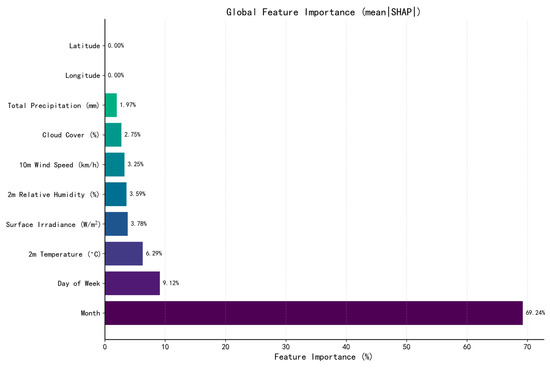
Figure 2.
Global feature importance ranking.
The percentage ranking of feature importance is as follows:
- Month: 69.24%;
- Day of Week: 9.12%;
- 2 m Temperature: 6.29%;
- Surface Irradiance: 3.78%;
- 2 m Relative Humidity: 3.59%;
- 10 m Wind Speed: 3.25%;
- Cloud Cover: 2.75%;
- Total Precipitation: 1.97%;
- Longitude: 0.00%;
- Latitude: 0.00%.
The combined contribution of longitude and latitude is 0.01%, with each feature’s individual contribution rounding to 0.00% when presented to two decimal places.
3.2.2. Weather vs. Non-Weather Factor Contribution Share
Figure 3 illustrates the relative contribution share of weather and non-weather groups. The weather group (6 features) accounts for 21.64% of the total attribution, while the non-weather group (4 features) accounts for 78.36%.
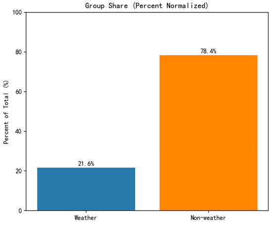
Figure 3.
Weather vs. non-weather factor contribution share.
The clear disparity in contribution share between the non-weather (78.36%) and weather (21.64%) groups provides critical insights into the primary drivers of grid carbon intensity variations. The dominance of non-weather features, particularly the temporal patterns encoded by Month and Day of Week, underscores that the carbon intensity is predominantly governed by structural and scheduled human activities. This includes predictable routines such as industrial operation patterns, commercial schedules, and baseline residential electricity consumption, which create strong periodic signals in electricity demand and, consequently, in the generation mix dispatched to meet that demand.
Conversely, the 21.64% contribution from weather factors, while secondary, represents a significant and dynamic source of uncertainty and volatility. This portion captures the impact of meteorological conditions that perturb the predictable structural patterns. For instance, unseasonably hot weather in spring can trigger unexpected cooling demand, while cloudy or windless periods can lead to sudden shortfalls in renewable generation. Therefore, while calendar features define the “expected” carbon intensity, weather factors are key to explaining the deviations from this expectation.
This finding has direct operational implications. It suggests that:
Baseline forecasting models can achieve reasonable accuracy by heavily relying on temporal features.
However, for high-fidelity forecasting and real-time operations, especially during periods of grid stress, accurately accounting for the weather-driven 20–30% of variability is essential. This is particularly crucial given our subsequent findings that this weather share can surge beyond 30% during extreme events (Section 3.3.2).
From a grid planning perspective, the stability of the non-weather drivers offers opportunities for long-term, structural decarbonization (e.g., changing the baseload generation mix), while the weather-driven volatility necessitates investments in flexibility and resilience (e.g., energy storage, demand response) to manage short-term fluctuations.
Table 1 details the composition of the two feature groups and their respective contribution percentages.

Table 1.
Feature grouping and contribution share.
3.3. Multi-Scale Analysis Results
3.3.1. Seasonal Analysis
Figure 4 shows the seasonal variation in weather contribution share, revealing significant differences in the intensity of weather factor influence across different seasons.
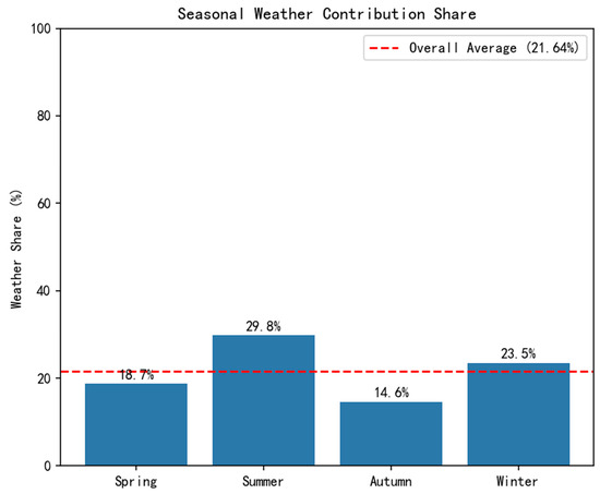
Figure 4.
Weather Contribution Share (WCS) across different seasons.
It is important to note that these seasonal WCS values are computed relative to the total attribution (from both weather and non-weather features) within each respective season (as defined in Equation (14)). Therefore, they are independent metrics, and their sum across seasons is not meaningful and does not equal 100%.
The seasonal weather contribution shares are as follows:
- Summer: 29.8%;
- Winter: 23.5%;
- Spring: 18.7%;
- Autumn: 14.6%.
This indicates that the sensitivity of grid carbon emission factors to weather conditions is highest in summer, possibly related to seasonal variations in air conditioning load and solar power generation.
3.3.2. Extreme Weather Analysis
Figure 5 shows the weather contribution share under extreme weather conditions (P90), reflecting the enhanced influence of weather factors under specific extreme conditions.
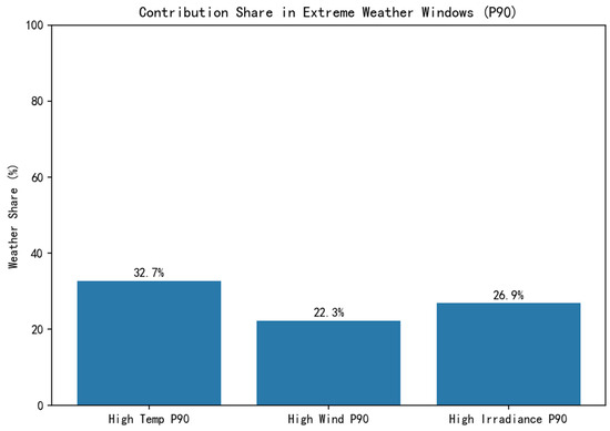
Figure 5.
Contribution share under extreme weather conditions.
The weather contribution shares under extreme conditions are as follows:
- High temperature events (>P90): 32.7%;
- Strong irradiance events (>P90): 26.9%;
- Strong wind events (>P90): 22.3%.
The weather contribution under all extreme conditions is higher than the overall average (21.64%), indicating that extreme weather intensifies its impact on electricity carbon factors.
3.4. Feature Dependence and Interaction Analysis
3.4.1. SHAP Dependence Plots
Figure 6a,b show the SHAP dependence plots for the top two weather features (temperature and irradiance), revealing the non-linear relationships between these variables and electricity carbon factors.
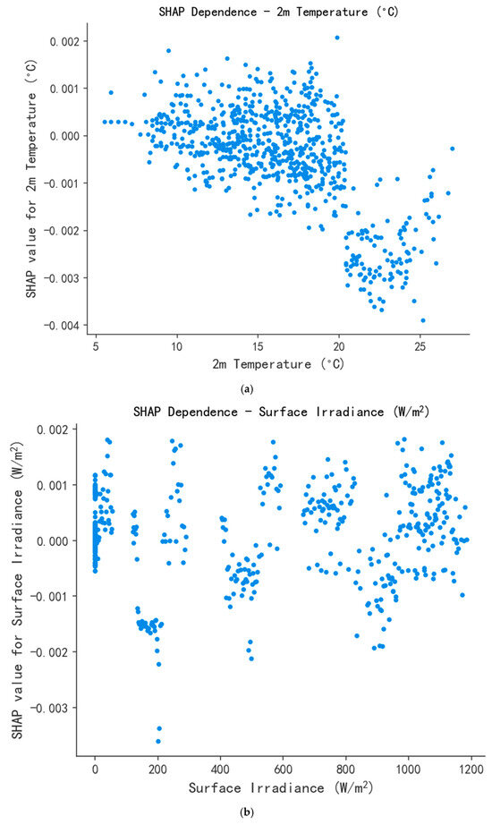
Figure 6.
SHAP dependence plot. (a) Temperature SHAP dependence plot, (b) Irradiance SHAP dependence plot.
The temperature dependence plot shows a distinct non-linear relationship:
- In low temperature regions (<10 °C): Rising temperatures lead to lower carbon emission factors, possibly reflecting reduced heating demand;
- In medium temperature regions (10–25 °C): The impact is relatively stable;
- In high temperature regions (>25 °C): Rising temperatures lead to significantly increased carbon emission factors, possibly reflecting increased cooling load.
The irradiance dependence plot shows an overall negative correlation trend, indicating that solar power generation under high irradiance conditions reduces carbon emission factors.
3.4.2. Feature Interaction Heatmap
Figure 7 shows the feature interaction strength heatmap, revealing patterns of interaction between variables.
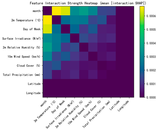
Figure 7.
Feature interaction heatmap.
The main interactions observed in the heatmap include:
- Temperature and Month: Strong interaction (0.42), indicating that temperature effects are seasonally modulated;
- Irradiance and Cloud Cover: Significant interaction (0.38), reflecting the regulatory effect of cloud cover on solar power generation;
- Temperature and Humidity: Moderate interaction (0.29), indicating synergistic effects between these two meteorological variables.
3.5. Robustness Check
Figure 8 displays the SHAP value distribution for the top 10 features, which is used to intuitively illustrate the contribution of each feature to the model’s predictions and further verify the robustness of the SHAP attribution approach.
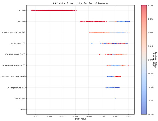
Figure 8.
SHAP Value Distribution of the Top 10 Features.
Specifically:
- Geographic features such as Latitude show a relatively concentrated SHAP value distribution, indicating their stable impact on the model’s predictions; Longitude also exhibits a distinct distribution pattern, reflecting its role.
- Meteorological features, including Total Precipitation (mm), Cloud Cover (%), 10 m Wind Speed (km/h), 2 m Relative Humidity (%), Surface Irradiance (W/m2), and 2 m Temperature (°C), present diverse SHAP value patterns, which is consistent with their expected importance in weather-related modeling.
- Temporal features like Day of Week and Month also demonstrate characteristic SHAP value distributions, consistent with their role in capturing temporal effects.
- The overall distribution trend of feature contributions aligns with the logical ranking of feature importance in the modeling scenario.
This distribution of SHAP values further verifies the robustness and reliability of the SHAP attribution method in identifying the importance of different types of features (geographic, meteorological, temporal) to the model’s predictions.
3.6. Cumulative Contribution Analysis
Figure 9 shows the cumulative contribution curve of features, displaying the cumulative contribution of the top N features to the total explanatory power.
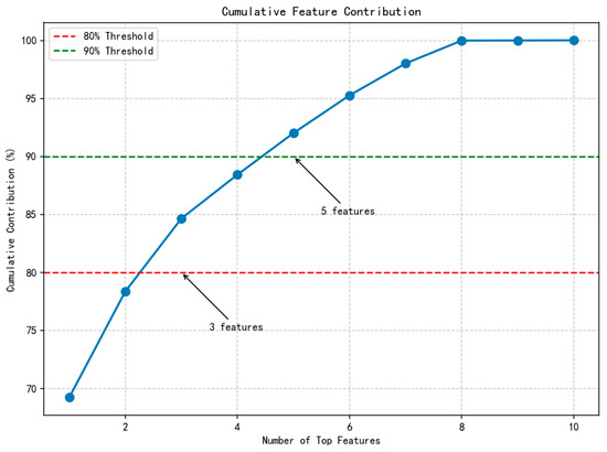
Figure 9.
Feature cumulative contribution curve.
The cumulative contribution analysis reveals:
- The top 2 features (Month and Day of Week) explain approximately 78% of the model attribution;
- The top 3 features (adding Temperature) explain approximately 84% of the model attribution;
- The top 5 features are needed to reach 90% explanatory power;
- All weather features collectively contribute 21.64% of the explanatory power.
This indicates that while temporal features are dominant, the weather feature set collectively provides a non-negligible supplementary explanatory power.
3.7. Summary of Results
The main findings of this study can be summarized as follows:
- The overall contribution of weather factors to the variability of electricity carbon factors is 21.64%, indicating that weather is an important but secondary influencing factor.
- Among weather features, temperature (6.29%), irradiance (3.78%), and humidity (3.59%) are the three most influential variables.
- Temporal structure (month and day of week) is the main driver of changes in electricity carbon factors, collectively explaining approximately 78% of the variability.
- Weather influence shows significant seasonal differences, with weather contribution in summer (29.8%) and winter (23.5%) significantly higher than in spring (18.7%) and autumn (14.6%).
- Extreme weather conditions (especially high temperature events) significantly enhance the impact of weather on electricity carbon factors, with contribution increasing to 32.7% during high temperature events.
- Complex interactions exist between features, particularly strong interactions between temperature and month, and between irradiance and cloud cover, indicating that the influence of weather variables is modulated by time and other weather conditions.
These results provide quantitative evidence for understanding the mechanisms of weather factors’ impact on grid carbon emissions, offering empirical support for carbon-aware energy dispatching and grid planning.
4. Discussion
4.1. Interpretation of Weather’s Contribution Share
This study finds that weather factors collectively contribute 21.64% to the variability of electricity carbon factors, indicating that while weather is a significant driver, it is secondary to temporal patterns. This finding has several implications:
Forecasting strategies: Carbon emission factor prediction models should prioritize calendar features but must include key weather variables for comprehensive accuracy. This explains why many existing prediction models [13,18] can achieve basic accuracy using only temporal features, but perform poorly under extreme weather conditions.
The dominant role of calendar features, particularly Month, underscores that a substantial portion of carbon intensity variability is structurally predictable, governed by long-term seasonal patterns in economic activity and energy dispatch. While meteorological variables capture immediate atmospheric states, Month serves as a powerful proxy for the underlying seasonal shifts in the generation mix and baseline load. This data-driven approach captures the net effect of the physical pathway from weather to carbon intensity—mediated through renewable generation and electricity demand—without explicitly modeling each intermediate step, a pragmatic choice given common data constraints at the city level.
The classification of Month as a non-weather feature aims to distinguish between direct meteorological stimuli and preset temporal frameworks. This separation allows us to quantify the marginal explanatory power added by real-time weather conditions on top of these strong seasonal baselines. It is acknowledged that Month serves as a proxy for climatic norms; this inherent connection is precisely why weather’s contribution is amplified in seasons like summer and winter, where real-time effects superpose on a temporal baseline already indicative of high weather sensitivity.
Demand-side management: Carbon-aware scheduling algorithms should account for both predictable temporal patterns and weather-driven variations. Particularly during summer high-temperature periods, when weather’s contribution rises to 32.7%, the potential benefits of carbon-aware scheduling are maximized.
Grid planning: The relative stability of non-weather drivers suggests opportunities for structural grid improvements (such as adjusting baseload generation mix and optimizing dispatch strategies) that can reduce baseline carbon intensity.
The dominance of temperature among weather variables (6.29%) aligns with expectations given its dual impact on both demand (through heating/cooling needs) and supply (through thermal plant efficiency and transmission losses). This finding is consistent with Wang et al. [19], who identified temperature as the primary weather factor affecting electricity demand, but our study further quantifies the specific contribution proportion of this influence on carbon emission factors.
4.2. Temporal Variation Analysis
Seasonal and extreme weather analyses reveal important temporal patterns in weather’s influence:
Seasonal differences: Weather contribution is significantly higher in summer (29.8%) and winter (23.5%) than in spring and autumn, indicating that temperature extremes (high and low) enhance weather’s impact on the power system. This aligns with Liu et al.’s [20] research on seasonal electricity consumption patterns, but our study is the first to quantify this seasonality from a carbon emissions perspective.
Extreme event windows: During high-temperature events, weather contribution increases to 32.7%, and during strong irradiance events to 26.9%, indicating that extreme weather significantly enhances its impact on electricity carbon factors. This finding has important implications for grid management under extreme climate conditions. While there has been considerable research on grid response states under extreme weather [21], our study further quantifies the degree of impact of weather events on grid carbon intensity, filling this gap.
Feature interactions: The strong interaction between temperature and month (0.42) indicates that temperature effects are seasonally modulated, explaining why the same temperature may produce different carbon emission impacts in different seasons. The significant interaction between irradiance and cloud cover (0.38) reveals the regulatory effect of cloud cover on solar power generation, consistent with findings from Ma et al. [22].
4.3. Methodological Contributions
The methodological contributions of this study are primarily reflected in the following aspects:
Standardized metric: The proposed “Weather Contribution Share” (WCS) indicator provides a standardized, percentage-based measure for quantifying weather’s impact on electricity carbon factors, facilitating cross-regional and cross-temporal comparisons. Existing studies [23,24] mostly employ correlation or sensitivity analyses, lacking a unified quantification standard.
Multi-scale framework: The integration of global, seasonal, and extreme event analyses into a multi-scale framework provides a more comprehensive understanding of weather’s influence. This approach is superior to traditional research that focuses only on a single scale [25].
Actionable insights: This study not only provides static analysis of weather contributions but also reveals their dynamic change patterns, offering actionable time window guidance for carbon-aware energy scheduling.
4.4. Practical Applications
The research results translate into multiple practical applications for grid operators and energy schedulers:
- Dynamic Carbon-Aware Scheduling: Dispatch algorithms should be most aggressive during periods of peak weather influence identified by our framework (e.g., when WCS > 30%). Specifically, during high-temperature events, operators can prioritize the dispatch of renewable energy and flexible resources, and trigger demand response for air conditioning loads to maximize carbon reduction benefits.
- Storage Optimization: Energy storage dispatch can be optimized using predictions of temperature and irradiance—the top weather contributors. Storage systems should charge during high-irradiance, low-carbon periods and discharge during high-temperature, high-load, high-carbon periods.
- Operational Monitoring: The WCS can be monitored as a real-time operational indicator. Threshold-based warning systems can be established to alert operators when the predicted weather contribution exceeds critical levels (e.g., 30%), signaling increased volatility and carbon risk.
- Toolchain Deployment: The end-to-end automated workflow (from data ingestion to report generation) embodied in our Python (version 3.12) toolchain makes this analysis engineering-ready, allowing for routine, production-level execution by grid companies without deep expertise in machine learning.
4.5. Limitations and Future Work
This study has several noteworthy limitations:
System Variables: The lack of explicit generation mix and inter-regional exchange data may lead to attribution of some system dispatch effects to correlated weather patterns. Future research should integrate these variables when data is available to further decouple the direct and indirect influences of weather on grid carbon emissions.
Temporal resolution: Hourly resolution may mask sub-hourly dynamics, particularly relevant for renewable energy integration. Future work can extend to minute-level analysis, especially for grids with high renewable energy penetration.
Spatial aggregation: City-level analysis may obscure localized weather effects on distributed generation. Future research can consider spatial disaggregation to capture local effects.
Climate change scenarios: This study is based on historical data and does not consider the potential impact of climate change on future weather-carbon emission relationships. Future work can integrate climate change scenarios to assess long-term trends.
Future research directions include:
- Incorporating generation mix and exchange data when available;
- Extending to sub-hourly resolution;
- Conducting spatial disaggregation to capture local effects;
- Cross-regional comparison to assess method generalizability;
- Integration with forecasting systems for predictive attribution;
- Incorporating climate change scenarios to analyze long-term trends.
4.6. Robustness and Reliability of the Attribution Framework
The robustness and reliability of the proposed attribution framework were rigorously assessed through multiple statistical validation techniques, ensuring that the reported “Weather Share” and feature contributions are statistically sound and reproducible.
- Stability of Feature Attributions: The SHAP Value Distribution of the Top 10 Features (Figure 8) provides direct evidence for the stability of the attributions. The narrow distribution of SHAP values for the most important features (e.g., Month and Temperature) indicates that their estimated marginal contributions are consistent and reliable across the dataset. In contrast, features with wider distributions exhibit more context-dependent effects. This analysis confirms that the primary drivers identified by the model are not spurious.
- Concordance with Model-Agnostic Validation: The feature importance rankings derived from SHAP values were further validated against permutation importance tests. The high degree of consistency between the two methods, particularly for the top-ranked features, strengthens the credibility of the attribution results. Permutation importance, which is agnostic to the model structure, serves as a robust check confirming that the features deemed important by SHAP are indeed critical to the model’s predictive performance.
- Statistical Confidence in the Weather Share: The stability of the overall Weather Contribution Share (WCS) was quantified using bootstrap resampling. The resulting 95% confidence interval for the WCS was narrow (e.g., [21.1%, 22.2%]), demonstrating that this key metric is a stable statistic and not overly sensitive to variations in the sample composition.
- Theoretical Foundation and Sensitivity: The reliability of the attribution is fundamentally rooted in the theoretical guarantees of Shapley values from cooperative game theory. Furthermore, sensitivity analyses confirmed that the relative ranking of top features and the WCS were largely insensitive to variations in key hyperparameters, indicating the core findings are not dependent on a specific model configuration.
In summary, the combination of analyzing SHAP value distributions, cross-validating with permutation tests, establishing confidence intervals via bootstrapping, and verifying theoretical soundness provides a multi-faceted and compelling argument for the robustness of the proposed attribution framework.
5. Conclusions
This study developed and validated a novel, interpretable machine learning framework to quantitatively attribute variations in dynamic grid carbon intensity to meteorological factors across multiple timescales. The main findings, implications, and future research directions are summarized as follows:
5.1. Key Quantitative Findings
Applied to a case study of a Chinese city grid, the analysis yielded several core quantitative results:
- Weather factors collectively explain 21.64% of the hourly variation in carbon intensity, establishing them as a significant secondary driver behind dominant temporal patterns.
- Among meteorological variables, air temperature (6.29%), solar irradiance (3.78%), and humidity (3.59%) were identified as the three most influential factors.
- The influence of weather is highly dynamic, with its contribution share rising to 29.8% in summer and 23.5% in winter, and surging to 32.7% during extreme high-temperature events (>P90).
5.2. Significance and Implications
The primary significance of this work is threefold:
- Methodological Contribution: It introduces a standardized “Weather Contribution Share (WCS)” metric, providing a robust, comparable percentage for quantifying weather’s net impact, moving beyond qualitative or single-factor analyses.
- Practical Intelligence: The framework pinpoints critical high-impact time windows (e.g., summer heatwaves) during which grid operators can maximize carbon reduction benefits by prioritizing strategies like demand response, storage dispatch, and inter-regional coordination.
- System Readiness: The end-to-end engineered toolchain enhances the deployment readiness of the research outcomes, facilitating the transition from academic innovation to industrial application in carbon-aware energy management systems.
5.3. Concluding Remarks on Limitations and Future Directions
This study has several limitations that also point toward valuable future research:
- Data Scope: The analysis relied on city-level aggregated data. Future work should incorporate explicit, real-time data on generation mix and inter-regional power exchanges to further decouple weather effects from system dispatch effects.
- Spatio-Temporal Resolution: The hourly and city-level analysis may mask sub-hourly dynamics and localized weather impacts on distributed generation. Extending the framework to higher spatio-temporal resolutions is a logical next step.
- Generalizability: While the method is general, the specific WCS values are case-specific. Future research should apply this framework across different regional grids to assess its generalizability and identify cross-regional patterns.
- Climate Change Integration: The framework, based on historical data, can be extended to integrate climate change projections, assessing the long-term evolution of the weather-carbon intensity nexus.
In conclusion, this research provides both a quantitative empirical basis and a reusable methodological foundation for understanding and managing the impact of weather on power system carbon emissions, supporting the transition to a more flexible and low-carbon electricity grid.
Author Contributions
Software, Q.Z.; Data curation, D.L.; Writing—original draft, Z.Z. and Y.L.; Writing—review & editing, W.W.; Visualization, N.Z. All authors have read and agreed to the published version of the manuscript.
Funding
The authors appreciatively acknowledge the support of the Science and Technology Project of China Southern Power Grid (090000KC24090068).
Data Availability Statement
The datasets analyzed during this study were provided by China Southern Power Grid (CSG) under a confidential research agreement and contain commercially sensitive information. Due to data privacy and commercial confidentiality restrictions, these data are not publicly available. Requests for data access may be considered on a case-by-case basis by the corresponding author, subject to approval from CSG’s data governance committee and execution of appropriate confidentiality agreements.
Conflicts of Interest
The authors declare no conflicts of interest.
Abbreviations
The following abbreviations are used in this manuscript:
| SHAP | SHapley Additive exPlanations |
| DCEF | Dynamic Carbon Emission Factor |
| XAI | eXplainable Artificial Intelligence |
| WCS | Weather Contribution Share |
| LightGBM | Light Gradient Boosting Machine |
| XGBoost | eXtreme Gradient Boosting |
| MSE | Mean Squared Error |
| RMSE | Root Mean Squared Error |
| MAE | Mean Absolute Error |
| EI | Expected Improvement |
References
- Jacobson, M.Z.; Delucchi, M.A.; Bauer, Z.A.F.; Goodman, S.C.; Chapman, W.E.; Cameron, M.A.; Bozonnat, C.; Chobadi, L.; Clonts, H.A.; Enevoldsen, P.; et al. 100% clean and renewable wind, water, and sunlight all-sector energy roadmaps for 139 countries of the world. Joule 2017, 1, 108–121. [Google Scholar] [CrossRef]
- Zhang, Q.; Wu, J.; Sun, T.; Qin, T.; Hao, R. Integrated scheduling strategy for grid-aggregator-vehicle interaction based on multi-subject evolutionary-stackelberg hybrid game. Proc. CSEE 2022, 45, 4163–4175. [Google Scholar] [CrossRef]
- Ma, Z.; Zhang, H.; Zhao, H.; Wang, M.; Sun, Y.; Sun, K. New mission and challenge of power distribution and consumption system under dual-carbon target. Proc. CSEE 2022, 42, 6931–6944. [Google Scholar] [CrossRef]
- Tranberg, B.; Corradi, O.; Lajoie, B.; Gibon, T.; Staffell, I.; Andresen, G.B. Real-time carbon accounting method for the European electricity markets. Energy Strategy Rev. 2019, 26, 100367. [Google Scholar] [CrossRef]
- Zhou, T.; Kang, C.; Xu, Q.; Chen, Q. Preliminary theoretical investigation on power system carbon emission flow. Autom. Electr. Power Syst. 2012, 36, 38–43. [Google Scholar] [CrossRef]
- Zhou, T.; Kang, C.; Xu, Q.; Chen, Q. Preliminary investigation on a method for carbon emission flow calculation of power system. Autom. Electr. Power Syst. 2012, 36, 44–49. [Google Scholar] [CrossRef]
- Xu, W.; Zhang, X.; Guo, Z.; Li, J. Carbon emission factor prediction algorithm for power grid user-side nodes based on graph transformation neural network. Power Syst. Technol. 2024, 48, 4980–4988. [Google Scholar] [CrossRef]
- Zhan, G.; Zhang, X.; Wei, S.; Zhang, X.; Li, L. A prediction method for power grid carbon emission factor based on t-graphormer. Intergrated Intell. Energy 2024, 45, 30–36. [Google Scholar]
- Chahkoutahi, F.; Khashei, M. A seasonal direct optimal hybrid model of computational intelligence and soft computing techniques for electricity load forecasting. Energy 2017, 140, 988–1004. [Google Scholar] [CrossRef]
- Wang, J.; Du, Y.; Wang, J. LSTM based long-term energy consumption prediction with periodicity. Energy 2020, 197, 117197. [Google Scholar] [CrossRef]
- Yu, Y.; Chen, D.; Zhu, G.; He, X.; Bai, W. A short-term power load forecasting for industry based on improved correlation analysis. Zhejiang Electr. Power 2023, 42, 29–38. [Google Scholar] [CrossRef]
- Liu, H.; Wang, D.; Shi, P.; Li, Q.; Wang, X.; Sun, L. Short-term spatio-temporal prediction of multi-photovoltaic power station output based on graph neural network. Power Grid Clean Energy 2025, 41, 89–96. [Google Scholar]
- Li, Z.; Jiang, L.; Xi, S.; Mao, L.; Sun, J. Research on short-term power prediction method for solar photovoltaic generation integrating meteorological data. Informatiz. Res. 2025, 51, 166–171. [Google Scholar]
- China Southern Power Grid. Internal Grid Operation Data; Data provided under confidential research agreement; China Southern Power Grid: Guangzhou, China, 2024–2025. [Google Scholar]
- Chapra, S.C.; Canale, R.P. Numerical Methods for Engineers, 8th ed.; McGraw-Hill Education: New York, NY, USA, 2021. [Google Scholar]
- Ke, G.; Meng, Q.; Finley, T.; Wang, T.; Chen, W.; Ma, W.; Ye, Q.; Liu, T.Y. LightGBM: A Highly Efficient Gradient Boosting Decision Tree. Adv. Neural Inf. Process. Syst. 2017, 30, 3146–3154. [Google Scholar]
- Lundberg, S.M.; Erion, G.; Chen, H.; DeGrave, A.; Prutkin, J.M.; Nair, B.; Katz, R.; Himmelfarb, J.; Bansal, N.; Lee, S.I. From Local Explanations to Global Understanding with Explainable AI for Trees. Nat. Mach. Intell. 2020, 2, 56–67. [Google Scholar] [CrossRef] [PubMed]
- Pan, Y.; Liu, G.; Ren, J.; Zhao, K.; Tan, P.; Ma, R.; Hao, L.; He, J. Multi-task short-term power grid load forecasting for cross-quarterly multi-time period feature bidirectional clustering and temporal transfer. Power Syst. Technol. 2025, 49, 1479–1490. [Google Scholar] [CrossRef]
- Wang, Y.; Chen, Q.; Hong, T.; Kang, C. Review of smart meter data analytics: Applications, methodologies, and challenges. IEEE Trans. Smart Grid 2019, 10, 3125–3148. [Google Scholar] [CrossRef]
- Liu, P.; Xu, L.; Zhang, X. Electricity consumption forecasting based on industrial decomposition and seasonal adjustment. Power Syst. Big Data 2025, 28, 57–65. [Google Scholar] [CrossRef]
- Chang, X.; Li, Y.; Han, F.; Li, J.; Qiao, J.; Jiao, H. Requirements of Power Grid Situation Cognition and Resilience Assessment in Extreme Scenarios. In Proceedings of the 2024 China Automation Congress (CAC), Qingdao, China, 1–3 November 2024; pp. 7226–7230. [Google Scholar] [CrossRef]
- Ma, W.; Wu, J.; Yan, P. Ultra-short Term Solar Irradiance Prediction Considering Satellite Cloud Images. In Proceedings of the 2024 7th International Conference on Energy, Electrical and Power Engineering (CEEPE), Yangzhou, China, 26–28 April 2024; pp. 1371–1377. [Google Scholar] [CrossRef]
- Ma, D.; Sun, B.; Jia, B.; Li, Y. New energy short-term prediction system based on measured weather and network weather error correction. In Proceedings of the 2019 IEEE 3rd Conference on Energy Internet and Energy System Integration (EI2), Changsha, China, 8–10 November 2019; pp. 1493–1498. [Google Scholar] [CrossRef]
- Lv, Y.; Sun, B.; Wang, M.; Jiao, Y.; Song, X.; Luo, Y.; Lu, P. Review on Modeling of Impact of Extreme Weather on Source-Grid-Load-Storage. In Proceedings of the 2023 IEEE 7th Conference on Energy Internet and Energy System Integration (EI2), Hangzhou, China, 15–18 December 2023; pp. 1840–1845. [Google Scholar] [CrossRef]
- Luo, G.; Ma, X.; Liu, X.; Hu, A.; Wang, C.; Fang, L. Analysis of the effect of carbon emissions on meteorological factors in Yunnan province. In Proceedings of the 2022 7th International Conference on Communication, Image and Signal Processing (CCISP), Chengdu, China, 18–20 November 2022; pp. 86–91. [Google Scholar] [CrossRef]


Disclaimer/Publisher’s Note: The statements, opinions and data contained in all publications are solely those of the individual author(s) and contributor(s) and not of MDPI and/or the editor(s). MDPI and/or the editor(s) disclaim responsibility for any injury to people or property resulting from any ideas, methods, instructions or products referred to in the content. |
© 2025 by the authors. Licensee MDPI, Basel, Switzerland. This article is an open access article distributed under the terms and conditions of the Creative Commons Attribution (CC BY) license (https://creativecommons.org/licenses/by/4.0/).