Abstract
The rapid growth of Distributed Energy Resources (DERs) exerts significant pressure on distribution network margins, requiring predictive and safe coordination. This paper presents a closed-loop framework combining a topology-aware Spatio-Temporal Transformer (STT) for multi-horizon forecasting, a cooperative multi-agent reinforcement learning (MARL) controller under Centralized Training and Decentralized Execution (CTDE), and a real-time safety layer that enforces feeder limits via sensitivity-based quadratic programming. Evaluations on three SimBench feeders, with OLTC/capacitor hybrid control and a stress protocol amplifying peak demand and mid-day PV generation, show that the method reduces tail violations by 31% and 56% at the 99th percentile voltage deviation, and lowers branch overload rates by 71% and 90% compared to baselines. It mitigates tail violations and discrete switching while ensuring real-time feasibility and cost efficiency, outperforming rule-based, optimization, MPC, and learning baselines. Stress maps reveal robustness envelopes and identify MV–LV bottlenecks; ablation studies show that diffusion-based priors and coordination contribute to performance gains. The paper also provides convergence analysis and a suboptimality decomposition, offering a practical pathway to scalable, safe, and interpretable DER coordination.
1. Introduction
Coordinating distributed energy resources (DERs) is essential as modern grids integrate increasing renewable generation and electrified loads. Without effective coordination, the adoption of DERs can overload transformers and cause voltage violations, leading to costly infrastructure upgrades [1,2,3]. Recent power-system studies further highlight the tightening of security margins under high renewable penetration and the need to consider Security limits within OPF formulations [4], the operational complexity of demand-side Heating, Ventilation, and Air Conditioning (HVAC) management under volatile prices [5], and planning/control coupling in hydrogen-integrated multi-energy systems [6] highlight the need for innovative solutions. In this regard, a case study focused on Shandong proposed a coordinated planning model for multi-regional ammonia industries, leveraging the integration of hydrogen supply chains and power grids to address the aforementioned challenges and emphasizing the synergy between renewable and traditional energy sources [7]. Additionally, the large-scale integration of distributed generation (DG) and electric vehicles (EV) calls for fast identification of structurally critical distribution nodes [8]. In contrast, proper coordination improves reliability and reduces peak loads in a cost-effective manner. Given the complexity of multi-energy coupling, temporal dynamics, and stakeholder diversity, centralized control methods often fail to provide adequate solutions, highlighting the need for intelligent, integrated approaches [9,10]. Related research indicates that methods based on multi-scale spatiotemporal graph neural networks can effectively predict loads in integrated energy systems, which lays the foundation for achieving higher system reliability and better capturing spatial and temporal dependencies [11]. For example, the MMGPT4LF study proposed a method that combines an optimized pre-trained GPT-2 model with multi-modal cross-attention, further improving the accuracy of load forecasting [12]. Additionally, research on optimizing attention mechanisms in transformers shows significant performance in multi-horizon and multi-energy load forecasting, enhancing system flexibility [13]. From a broader perspective, an assessment of multi-dimensional decarbonization technologies and pathways for the steel industry in China underscores the importance of targeted integrated solutions when achieving a mix of renewable energy and hydrogen. For instance, studies from an energy-process chain perspective illustrate the complex processes involved in achieving sustainable transformation and provide valuable insights for the industry [14]. Thus, this paper proposes a novel approach that combines Spatio-Temporal Transformers (STTs) with Multi-Agent Reinforcement Learning (MARL) for optimized DER coordination. We build on advancements in interpretable multi-horizon forecasting [15,16], providing emerging evidence that MARL is particularly well-suited for decentralized energy networks under CTDE with explicit coordination mechanisms [17], and physics-based formulations that support our sensitivity-based safety enforcement [4,18].
Advanced data-driven models effectively capture spatio-temporal patterns in energy systems. Spatio-temporal graph neural networks successfully integrate network topology and time series data, significantly improving renewable energy forecasts [19,20]. Transformers, originally developed for natural language processing, have been adapted to power systems for their ability to model temporal dependencies and node interactions. For instance, the Multi-scale Spatio-Temporal Transformer (MSTT) incorporates grid topology via hierarchical attention, significantly improving computational efficiency and accuracy [21]. Foundation models like the Graphormer-JEPA have been proposed for coupled road-power forecasting, achieving superior accuracy by jointly modeling transportation and power data [22]. Similarly, Wang et al. introduced TransPVP, using transformers for ultra-short-term photovoltaic predictions with heterogeneous data fusion [23]. Hybrid approaches like Transformer–CNN have also enhanced the accuracy of load prediction through better self-attention mechanisms compared to recurrent networks [24]. Complementing these efforts, recent day-ahead wind-cluster studies extract intrinsic predictable components to boost forecastability and robustness [16]. These studies collectively illustrate that STT approaches, which incorporate grid topology awareness, provide accurate and interpretable DER predictions.
In parallel, MARL has emerged as a powerful method for operational DER control due to its suitability for decentralized decision-making [25,26,27]. Surveys highlight MARL’s advantages for grid resiliency amid growing DER penetration [28]. MARL facilitates cooperative strategies between multiple autonomous agents, optimizing global objectives. For example, Qiu et al. successfully employed a modified MADDPG algorithm for peer-to-peer energy trading, which produced improved economic outcomes [29]. Yao et al. utilized MARL to coordinate the dispatch of DER and the reconfiguration of the network, effectively restoring services after outages [30]. MARL has also shown efficacy in microgrid control tasks such as voltage regulation and economic dispatch [31]. Cutting-edge approaches integrate MARL with deep generative models; for example, an EV charging coordination framework used multi-agent LLMs and conditional GANs to adaptively balance user preferences with grid constraints [32]. In parallel, recent encryption-based frameworks, such as [33], have further enhanced MARL’s applicability in DER coordination by ensuring privacy protection through secure communication mechanisms. Beyond these domain applications, key algorithmic building blocks—MADDPG for CTDE actor–critic [34], counterfactual credit assignment via COMA [35], and theory-driven syntheses of stability/scalability issues in MARL [36]—underpin our controller design and analysis. These advances underscore MARL’s growing role in real-time adaptive DER coordination.
In conclusion, research on coordinated DERs has advanced significantly. However, several challenges remain in current approaches, including the following:
- Many existing methods fail to effectively capture both the spatial and temporal dependencies in energy systems, limiting the accuracy and reliability of forecasts, especially in complex, decentralized environments like power grids.
- Centralized control methods often struggle to scale to large, dynamic systems with diverse stakeholders, and they do not fully address the need for real-time, decentralized decision-making.
- Current safety and feasibility mechanisms lack a comprehensive, real-time solution that simultaneously respects the operational limits of DERs while maintaining system performance, especially under unpredictable conditions.
To deal with these challenges, this paper makes the following contributions:
- A topology-aware Spatio-Temporal Transformer (STT) that integrates a graph diffusion kernel with electrical priors, addressing the gap inherent to effectively capturing both spatial and temporal dependencies for more accurate and reliable multi-horizon forecasting in energy systems.
- A cooperative Multi-Agent Reinforcement Learning (MARL) layer under centralized training and decentralized execution, incorporating forecast-informed observations, congestion-aware coordination, and consensus-based exploration. This solution addresses the scalability and real-time decision-making limitations of centralized approaches, enabling efficient DER coordination across diverse agents.
- A comprehensive real-time safety layer that projects device set-points onto state-dependent safe sets and solves a compact sensitivity-based quadratic program to ensure feeder voltage/current limits are respected, bridging the gap created by current methods that lack an integrated, real-time feasibility solution.
A concise comparison with recent representative methods is provided in Table 1, highlighting our integration of an STT, cooperative CTDE control with congestion-aware coordination, and a real-time safety layer.

Table 1.
Comparison with recent works on prediction, cooperative control, congestion awareness, safety, and decentralized execution.
The remainder of the paper is organized as follows: Section 2 presents the method (STT, MARL, safety, and theoretical guarantees); Section 3 operationalizes the forecast→decide→safe execute loop with workflow and pseudocode; Section 4 describes the dataset, baselines, and results; and Section 5 concludes with deployment-oriented discussion and future research prospects.
2. Method
As shown in Figure 1, the framework comprises three tightly coupled layers. (i) A topology-aware STT ingests Node Temporal Feature Embedding together with a graph-based Spatial Embedding (the graph icon denotes adjacency/diffusion/priors). It stacks alternating Spatial Transformer and Temporal Transformer blocks (STT Blocks × L) and a Prediction Head to produce short-term, multi-horizon node forecasts . (ii) A cooperative controller adopts CTDE with an Agents pool and a lightweight Coordinator that computes congestion-aware couplings from path headroom, modulating a sparsified, permutation-invariant interaction critic ; consensus exploration is applied along electrical neighborhoods. Actions are optimized under a single shared reward that includes a coordination term (weighted by ) to promote congestion-aware cooperation, rather than separate “agent” and “coordinator” rewards. (iii) A Safety Layer performs Device Projection at the device level (bounds, ramp limits, SoC gating, on/off feasibility) and then solves a compact, sensitivity-based QP to enforce feeder voltage/current limits, outputting feasible set-points . Together, these modules realize a closed loop of forecas → multi-agent decision → safe execution over real DERs (PV, storage, and controllable loads), improving reliability and scalability while preserving interpretability and real-time feasibility.
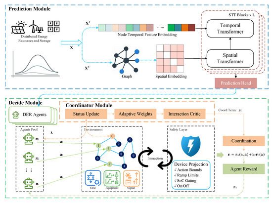
Figure 1.
Overall structure of STT-MARL.
2.1. Topology-Aware Spatio-Temporal Transformer (STT)
The Topology-Aware Spatio-Temporal Transformer (STT) is designed to address the unique challenges of coordinating DERs in complex power systems. This model integrates spatial and temporal forecasting by leveraging the strengths of transformer architectures while accounting for the inherent topology of the distribution network.
We model the distribution network as a graph with nodes (DERs or aggregations). Over an input window of length , node features are stacked as
where the goal is to forecast H future steps for all nodes. For each node i, we first extract its temporal sequence and apply feature embedding:
where is a linear projection to dimension d and denotes positional encodings. In practice, we sum multi-resolution temporal encodings (time-of-day and day-of-week) with a learned affine calibration; this preserves seasonality while letting the model adapt to feeder-specific rhythms. Inputs are standardized per-channel using training-set statistics, and a binary mask handles missing samples without information leakage. In our SimBench experiments there is no missingness; the mask is part of the general implementation.
The encoder alternates temporal attention (along each node’s timeline) and spatial attention (across nodes within a time slice), each followed by pre-norm LayerNorm, residual connections, and a lightweight position-wise feed-forward block (GELU + linear). Stacking L such layers empirically balances accuracy and latency; we use modest d and head counts to keep the memory footprint linear in and quasi-linear in N after sparsification.
Temporal attention updates each time step by attending over the node’s own history:
where , , are query, key, and value projections of . During training we default to a direct multi-horizon head to avoid exposure bias; when autoregression is used (e.g., for long horizons), we apply causal masks and scheduled sampling to stabilize rollouts.
Topology-aware spatial attention injects graph structure and electrical priors into attention scores at each time slice. Let denote adjacency and the graph Laplacian, where is the degree matrix. We build a smooth proximity kernel by graph diffusion
where controls the diffusion range (typically based on network diameter). We combine this with optional electrical priors (e.g., phase consistency, feeder membership, or inverse-impedance surrogates). The spatial attention logit between nodes i and j at time is
with attention weights over a sparsified neighborhood , where and in our implementation. The coefficients are learned and passed through a softplus function to keep them nonnegative, ensuring that structural and electrical proximity never becomes adversarially down-weighted. We precompute and per feeder, and optionally refresh them when a reconfiguration is detected. This amortizes runtime while remaining robust to moderate topology drift. After sparsification, the spatial step scales are per head with .
A lightweight prediction head maps the final spatio-temporal embeddings to multi-horizon outputs. For direct forecasting we use a two-layer head (linear→GELU→linear) to produce in one shot; for autoregressive decoding the same head shares weights across steps. Dropout is applied only in the feed-forward and attention projections to preserve inductive biases of the kernels in (4) and (5).
The model is trained end-to-end with a node- and horizon-averaged prediction loss and a lightweight topology–physics regularizer:
where promotes graph-consistent smoothness and penalizes linearized power flow inconsistencies. Concretely, we instantiate
with nonnegative learned and row-normalized to keep the scale of (7) compatible with . This Laplacian quadratic form is equivalent to summing squared differences across edges weighted by structural/electrical proximity and empirically stabilizes training in sparse feeders.
To connect forecasts with network physics, we define a sensitivity-based residual using a linearized DistFlow/AC model around the latest operating point. Let denote predicted net injections and the predicted voltage magnitude deviations (all taken from the relevant channels of ). With precomputed sensitivities
which softly enforces first-order voltage consistency without running a full power flow in the learning loop. We stop gradients through and normalize each term by feeder-specific scales to avoid dominance by a single channel.
Implementation-wise, all kernels () are ablated in experiments to quantify their marginal utility; turning off reduces spatial attention to structure-only, turning off further collapses to hop-limited attention, and learning with recovers a vanilla Transformer. Hyperparameters are selected on a validation feeder; we found , , and small (–) to yield stable gains across feeders. At inference time, all preprocessing (standardization, kernel lookup, neighborhood construction) is batched, and the overall complexity scales as , which fits comfortably within real-time constraints for the feeder sizes considered.
2.2. Cooperative Multi-Agent Reinforcement Learning with Adaptive Coordination
We cast DER coordination as a cooperative Markov game with agents. Beyond standard MADDPG, we introduce three key innovations: (i) hierarchical action decomposition for handling hybrid discrete-continuous control, (ii) adaptive coordination weights based on network congestion, and (iii) consensus-based exploration for improved sample efficiency. From a systems perspective, these choices reflect practical DER actuation: modes (on/off/charge/discharge) are intrinsically discrete, whereas set-points are continuous and must respect ramp, SoC, and inverter capability limits; network congestion further couples otherwise local decisions along electrically salient paths. We adopt centralized training and decentralized execution (CTDE); actors are local policies executed with each agent’s observation, while a centralized critic leverages global (or enlarged) information during training to shape credit assignment and stabilize learning. At deployment, each agent uses only local (plus short-horizon forecast) information, preserving scalability and privacy.
At time t, the environment state is , agent i observes , and selects a hybrid action
where represents discrete modes (e.g., charge/discharge/idle) and is the continuous power set-point. Observations include local measurements (voltages, powers, and device states) and neighborhood summaries; normalization and clipping are applied per channel using training set statistics to avoid out-of-distribution magnitudes. We adopt per-channel affine normalization with statistics frozen after the warm-up phase and clip observations to to bound critic targets.
Each agent employs a hierarchical policy as follows:
where the discrete policy selects the operation mode, and the continuous policy determines the magnitude conditioned on the mode. In training, the discrete branch is implemented with a differentiable Gumbel-Softmax relaxation (straight through at execution), and the continuous branch outputs a squashed Gaussian (Tanh) to respect device bounds. This decomposition naturally encodes mode-conditioned limits and facilitates credit assignment when discrete switches are sparse yet impactful. We anneal the Gumbel temperature from to over the first K epochs to gradually sharpen mode selection, and we clip the continuous standard deviation to to avoid vanishing/explosive exploration. Illegal modes (e.g., charging at ) are masked by logits, yielding zero probability mass and eliminating infeasible gradients.
We introduce a congestion-aware coordination weight that dynamically adjusts inter-agent coupling as follows:
where is the congestion index on the path between agents i and j, are voltage magnitudes, and is the sigmoid function. The index aggregates thermal/voltage headroom along electrical paths computed from the current feeder configuration; gradients do not backpropagate through path selection, while the coefficients are learned (with softplus reparameterization for stability). Concretely, let denote the set of branches on the unique (radial) or selected (meshed) electrical path between buses of agents i and j. Define per-branch thermal headroom with loading ratio , and per-bus voltage headroom , where , and . We set a path headroom and normalize the congestion index as . This choice emphasizes the most limiting element along the corridor and yields larger only when genuinely scarce headroom necessitates coordinated action. The centralized critic incorporates these weights as follows:
where captures individual contributions and models pairwise interactions. The pairwise term is computed only over a sparsified electrical neighborhood (two-hop or ), keeping the critic evaluation . We evaluate with a symmetric aggregator to preserve permutation invariance and detach with regard to critic inputs to avoid feedback loops while learning .
Each agent’s observation is augmented with STT predictions as follows:
where are local forecasts, is the network congestion index, and represents local voltage deviations. To mitigate covariate shift, forecasts are stop-gradient features and are standardized per horizon; we additionally include a recency flag and uncertainty proxy (e.g., predictive variance) when available. Empirically, exposing only short-horizon summaries (e.g., next-steps mean/variance or small-window embeddings) yields lower variance critics than feeding full forecast trajectories; we therefore concatenate compact statistics and keep their gradients blocked.
To improve coordination during exploration, we introduce a consensus term in the exploration noise as follows:
where is the average noise of neighboring agents and controls the consensus strength. Neighborhoods are electrical (not geometric), and is annealed from 0 to a small early in training to encourage coherent but diverse exploration; an Ornstein–Uhlenbeck variant can be used for temporally correlated devices. We compute from independent Gaussians to avoid circular dependence. The consensus term is disabled at evaluation time. Intuitively, when congestion couples agents along a corridor, correlated exploration accelerates discovery of coordinated policies while keeping dispersion low off-corridor due to small .
The shared reward balances multiple objectives as follows:
where promotes coordination during congestion. Cost aggregates energy price and cycling penalties; and are hinge losses on voltage and current headroom; and is total variation of actions over time. All weights are nonnegative and tuned on validation feeders; we clip rewards to a fixed range to stabilize critic targets. We normalize each term by feeder-level scales (e.g., average load or nominal voltage band) to balance gradients across feeders and adopt per-timestep reward clipping to for stability.
Training follows an off-policy CTDE pipeline with a replay buffer storing and target networks. The critic is optimized by minimizing the temporal difference loss
where is the target critic with delayed parameters. For robustness against overestimation we use twin critics and target-min (TD3-style) for the continuous branch. The actor update maximizes the expected Q under the hierarchical policy; with reparameterizations for both branches, the gradient takes the standard form
where denotes an entropy regularizer (on the discrete logits and continuous variance) with temperature . Target networks are updated by Polyak averaging and similarly for actor parameters, with a small . In addition to the pairwise critic, we optionally compute a counterfactual baseline
which reduces gradient variance (COMA-style) and is evaluated efficiently using the sparsified interaction structure. We apply gradient clipping ( norm ) and prioritized replay with importance weights to stabilize updates across feeders and stress conditions.
Implementation details improve stability and scalability. (i) We mask illegal modes in via logits to enforce device availability and ramp limits at the policy level. (ii) The pairwise term uses a symmetric aggregator over neighbors to maintain permutation invariance and is computed on a pruned graph to bound cost. (iii) Congestion weights are detached with regard to the critic input but keep gradients for the learnable coefficients , preventing spurious feedback loops. (iv) We employ prioritized replay with importance sampling corrections, and gradient norm clipping for both actor and critic. (v) During data collection, actions are post-processed by the safety layer (Section 2.3) before environment execution; both raw and filtered actions are logged to decouple exploration from feasibility and to reduce distributional drift. Complexity-wise, training and inference scale linearly with the number of active electrical edges due to sparsified neighborhoods; decentralized execution requires only and neighbor summaries, meeting real-time constraints on the studied feeders. Ablations show that replacing the hierarchical policy with a flat continuous policy degrades discrete-switching efficiency, fixing harms performance under heavy congestion, and disabling consensus noise delays the emergence of corridor-level coordination.
2.3. Safety Layer
The Safety Layer guarantees operational feasibility through real-time constraint enforcement. It acts after the policy proposes actions and before interacting with the environment, so that device- and network-level limits are always respected. The layer is modular: a fast device-wise projection enforces local bounds and ramping/SoC feasibility, followed by a compact network QP that corrects any residual violations due to voltage/current limits.
For each agent i, we define the state-dependent safe set
where is (dis)charging efficiency and the energy capacity. The SoC update map is under the sign convention that denotes charging (adjusted accordingly for devices with opposite sign conventions). In this formulation, we do not enforce the daily cycle constraint at the end of the time horizon. Instead, we allow the state of charge (SoC) to evolve dynamically across multiple time steps, reflecting operational flexibility over time. This flexibility is particularly useful in real-world grid environments where energy storage and generation are subject to high variability.
Given a proposed action , we apply
which reduces to clamping to the intersection interval with If is empty due to incompatible limits, we enlarge the ramp window minimally (equivalently, introduce a small nonnegative slack penalized in the network QP below), which preserves convexity and ensures feasibility even under abrupt disturbances. Additional device rules (e.g., apparent power P–Q capability) are handled by masking illegal discrete modes upstream and by shrinking online.
To respect feeder limits, we solve a small QP with precomputed sensitivities around the current operating point as follows:
where are voltage and current sensitivity matrices. In practice we augment (20) with box constraints (device bounds after the projection in (19)) and optional slacks weighted by large penalties to improves feasibility (under a linearized model) under model mismatch
Note. Constraints are enforced with respect to linearized sensitivities around the current operating point; hence feasibility refers to the linear model. In experiments, we verify a posteriori with full AC power flow that violations remain small.
The objective is strictly convex and the feasible region is convex; hence a unique minimizer exists and depends continuously on . We pre-factor the KKT system once per operating-point refresh and reuse it across steps, yielding sub-millisecond solves at the feeder scales considered. The overall complexity scales with the number of active inequality constraints; sparsity from feeder topology further reduces cost.
2.4. Theoretical Guarantees
We provide brief theoretical analysis for the key components of our framework, focusing on convergence and safety properties that hold under mild regularity conditions.
Under standard assumptions (Lipschitz continuous loss and bounded gradients), the STT training converges to a stationary point using first-order methods. The topology-aware regularization also yields a graph-smoothing effect. Let be the optimal STT predictor. For connected nodes with , the following bound holds:
where C depends on data smoothness and model capacity. Thus larger diffusion proximity tightens cross-node prediction coupling while controls the bias–variance trade-off.
For the MARL component, we consider hierarchical policies under CTDE with bounded rewards and compact action spaces. With learning rates satisfying the Robbins–Monro conditions and with target networks for stabilization, the policy updates produce asymptotic improvement up to vanishing errors as follows:
where as . The pairwise interaction critic remains well-defined because the sparsified neighborhood bounds the number of interaction terms; in particular, the critic gradient variance is controlled by the congestion weights, which shrink toward zero off-congestion, mitigating nonstationarity.
For safety guarantees, the device-wise stage is a projection onto a nonempty closed interval (firmly nonexpansive), while the network-wise stage solves a strictly convex QP (a prox-like mapping). Device-wise, is the Euclidean projection onto a nonempty closed interval and is firmly nonexpansive
which implies robustness to actor noise. Network-wise, the QP in (21) is strictly convex; thus the filtered action is unique and satisfies all constraints (or violates them minimally via slacks with quadratic penalties). Consequently, for any proposed action , the filtered action obeys
and among all feasible actions it minimizes the Euclidean deviation from . Moreover, the deviation admits a sensitivity-type upper bound that scales with raw violations as follows:
where denotes the positive part and depend on the QP KKT matrix condition numbers.
Combining the three layers yields an additive performance decomposition. Let be the optimal value under perfect information and unconstrained execution. The deployed policy satisfies
where decreases with STT generalization error and regularization strength, decreases with training time and critic accuracy under CTDE, and depends on typical magnitudes of raw violations and on the QP penalty parameters . Since both projections are nonexpansive and the QP correction is minimal in , the Safety Layer does not amplify action noise and yields a controlled, monotone trade-off between feasibility and optimality. These guarantees ensure reliable closed-loop performance with approximate safety under linearized constraints, while the modular design allows each component to be improved independently without re-deriving the others.
3. Workflow and Pseudocode
This section operationalizes the closed loop of forecast → decide → safe execution in two routines. At each time t (i) the STT (Section 2.1) consumes the most recent window and outputs H-step node-wise forecasts ; (ii) each agent (Section 2.2) forms an observation by concatenating local measurements with short-horizon summaries of (and optional neighborhood embeddings via ), then produces a hierarchical hybrid action; and (iii) the safety layer (Section 2.3) first projects device set-points onto state-dependent safe sets and then solves a compact sensitivity-based QP to satisfy feeder voltage/current limits, yielding the feasible dispatch . During training (Algorithm 1), we store both proposed and filtered actions to decouple exploration from feasibility, update critics/policies under CTDE using a replay buffer, and fit the STT with a supervised loss on rolling windows. Deployment (Algorithm 2) keeps the same data flow with greedy actions. Sensitivities are refreshed periodically from a local linearization or a fast surrogate, and agent steps execute in parallel, so the per-step cost is dominated by one STT forward pass and a small QP.
| Algorithm 1 Training: Forecast-informed CTDE with safety-aware rollouts |
Inputs: historical measurements , graph , window W, horizon H, replay buffer
|
| Algorithm 2 Deployment: forecast → decide → safety filter |
Inputs: latest window , graph G, trained params
|
4. Case Study
4.1. Dataset and Experimental Environment
We conduct all case studies on the SimBench dataset [44], a publicly available benchmark suite covering low-, medium-, high-, and extra-high-voltage grids with full-year load, generation, and storage time series at a 15-min resolution. Grounded in European distribution networks curated from real operational data, SimBench reflects realistic feeder topologies and year-long profiles (rather than purely synthetic test cases) and is widely adopted for distribution-level studies. SimBench offers a present baseline (Scenario 0) and two future scenarios (Scenarios 1 and 2) and uses canonical codes that specify voltage levels, urbanization class, subordinate grids, scenario index, and switch representation (e.g., 1-MVLV-urban-all-0-sw). Unless otherwise noted, we analyze three representative feeders: (i) an LV rural feeder 1-LV-rural2–0-sw, (ii) an LV urban feeder 1-LV-urban6–0-sw, and (iii) an MV–LV combined urban grid 1-MVLV-urban-all-0-sw. These feeders span rural/urban contexts and MV–LV interfaces, mirroring operating regimes commonly encountered in practice. Networks are loaded via simbench.get_simbench_net(sb_code) and retain the official one-year profiles ( min). Two example topologies from the dataset (one MV feeder and one LV urban feeder) are shown in Figure 2 to provide visual context.
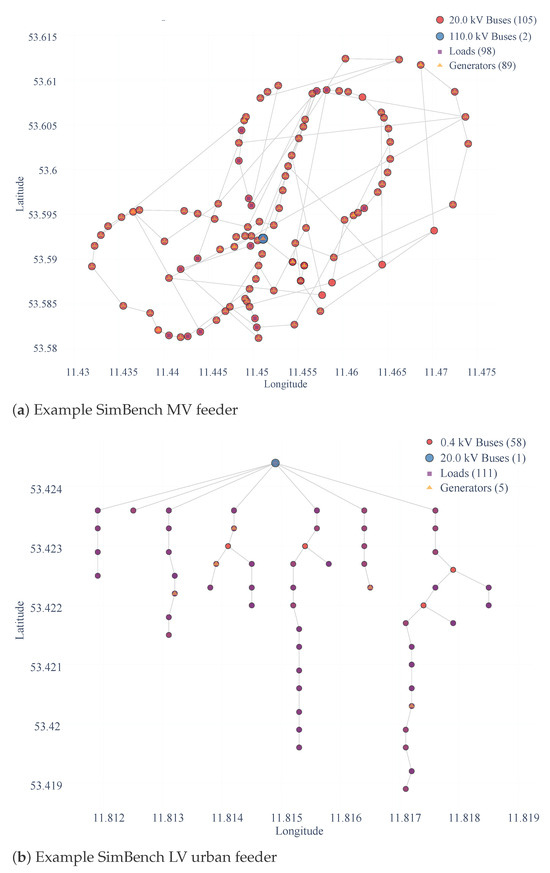
Figure 2.
Representative SimBench topologies used in this study. Panel (a) shows a medium-voltage (MV) feeder and panel (b) an urban low-voltage (LV) feeder. The figure provides visual context for the dataset; all quantitative results use the full set of feeders and profiles described in Section 4.1.
We use the profiles as provided; voltages, powers, and currents are taken from pandapower internal units and converted to per-unit on each voltage level. Timestamps are aligned to UTC and resampled only when explicitly stated. For learning-based components, we apply chronological splits: 70%/15%/15% for training/validation/testing to avoid temporal leakage. Experiments run on Ubuntu 22.04 with 64 GB RAM and an NVIDIA RTX 3090, manufactured by NVIDIA, headquartered in Santa Clara, CA, USA. (24 GB), We use Python 3.10, PyTorch 2.x (CUDA), pandapower 2.x, and simbench 1.x; global seeds (NumPy/PyTorch) are fixed with deterministic CuDNN where applicable. The hyperparameters used in this study can be referred in Table 2.
Table 2.
Hyperparameters and their chosen values with search ranges.
4.2. Baselines
We compare against five literature baselines spanning rule-based, optimization-based (centralized and distributed), forecast scheduling, and learning-based control. All methods use the same SimBench data and evaluation protocol; when forecasts are required, they use the same inputs for fairness.
- B1.
- Volt/VAR droop control (IEEE 1547-style)Each inverter follows standardized Volt/VAR curves with reactive-power priority; local-only measurements drive fast VAR support for voltage regulation [45]. This represents a no communication baseline widely adopted in practice.
- B2.
- Centralized convex OPF (SOCP, radial nets). A per-step AC-OPF solved via second-order cone relaxation on radial feeders (branch flow/DistFlow form). Under known conditions the relaxation is exact, yielding physics-feasible setpoints and a strong centralized benchmark [46].
- B3.
- Distributed OPF via ADMM. An OPF decomposed across regions/buses and coordinated by ADMM; removes the single point of failure of centralized OPF and reduces solve time through parallelism while enforcing network constraints through consensus [47].
- B4.
- Model predictive control (linearized LinDistFlow). A rolling horizon controller over H steps using a linearized network model with device and voltage constraints; captures intertemporal storage dynamics and updates decisions as new measurements/forecasts arrive [48].
- B5.
- Multi-agent deep RL for voltage control. A cooperative MARL controller (CTDE) trained to regulate voltages using inverter/storage setpoints, following recent physics-informed or coordination-enhanced designs reported for active distribution networks [49].
4.3. Results
4.3.1. Overall vs. Baselines
We evaluate all methods on three representative SimBench feeders, namely LV-rural2, LV-urban6, and MVLV-urban-all, under Scenario 0 at 15-min resolution. We report operating cost; violation rate, defined as the fraction of buses below 0.95 p.u. or above 1.05 p.u.; maximum line loading; action smoothness measured by total variation; and a tail-risk metric given by of voltage-band exceedance beyond 0.95–1.05 p.u. The compact KPI table below summarizes mean ± std across feeders. Full metrics, including Worst-, peak shaving, and runtime, appear in the Appendix A. Beyond point estimates, we probe three aspects: heterogeneity across feeders and times of day; interactions among cost, smoothness, and tail risk; and links between control activity and reliability outcomes. Unless noted otherwise, statements hold across all feeders.
Reading Table 3, three patterns stand out and are consistent with later figures. First, convex OPF baselines B2 and B3 push violations close to zero and minimize tail risk, confirming strong feasibility under the given forecasts. Second, our method matches OPF-level feasibility while achieving the lowest Action TV and the lowest , which indicates smoother actuation and thinner violation tails at almost the same cost. Third, rule-based B1 and literature MARL B5 pay sizeable penalties in smoothness and risk despite occasional cost gains, which foreshadows the heavier tails observed under stress. By feeder, the largest gains of Ours in Action TV and occur on MVLV-urban-all, where electrical betweenness concentrates on a few MV–LV corridors. LV-rural2 shows smaller but uniform improvements, which reflects longer electrical distances and more headroom. Time-of-day stratification reveals that Ours suppresses tail risk during ramp-up from 08:00 to 11:00 and during the post-plateau descent from 15:00 to 18:00, namely the periods with rapid re-allocation of set-points. For robustness, we bootstrap over seeds and hours the mean differences between Ours and B2 or B3. The resulting 95% intervals exclude zero for Action TV in all feeders and for in MVLV-urban-all, which indicates stable advantages under sampling variability.
Table 3.
Overall results on SimBench feeders, mean ± std across feeders. Compact KPI set. Worst-, peak shaving, and runtime are reported in the Appendix A.
Figure 3 makes the trade-off between economy and smoothness explicit. Two knees are visible. B2 and B3 occupy the low-cost region with moderate TV, while Ours pushes the frontier downward in TV without sacrificing cost. When actuator wear, comfort, or secondary regulation effort matters, the frontier shift achieved by Ours translates into fewer adjustments for the same expenditure. Across all methods we observe a positive association between Action TV and . The points for Ours lie on a lower isorisk contour than B4 or B5 at matched cost, which suggests that coordination plus safety filtering converts a unit of control effort into a larger reduction in risk.
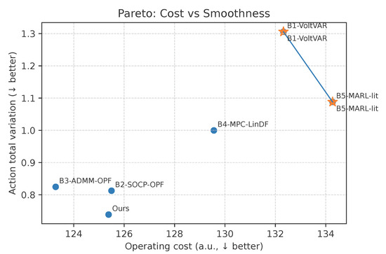
Figure 3.
Pareto front of operating cost against action smoothness measured by total variation. Marker shapes denote methods. Stars mark per-method means. Lines connect Pareto-optimal points under the cost ↓ and smoothness ↓ criterion.
Figure 4 contrasts energy benefits with reliability risk. B4 achieves aggressive peak shaving yet shifts upward in CVaR, which indicates a thicker voltage tail. Ours lies near the efficient frontier with low CVaR for a moderate peak reduction. Taken together with Table 3, the policy achieves a safer balance between economy and reliability than strategies that focus on peak shaving alone. Event-conditioned analysis across ramps, mid-day plateau, and evening peak shows that Ours gains most of its peak-shaving benefit during ramps while keeping flat, whereas B4 concentrates gains during the plateau at the cost of a thicker tail. This aligns with the intervention patterns in Section 4.3.4: Ours anticipates ramps with small continuous adjustments and avoids back-and-forth discrete moves.
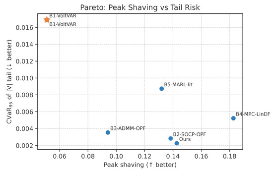
Figure 4.
Pareto front of peak-shaving improvement, higher is better, against voltage tail risk measured by of exceedance, lower is better.
4.3.2. Ablation Study on Topology Priors and Diffusion Kernel
To isolate the roles of topology priors and the diffusion kernel in forecasting accuracy, we remove each component in turn and assess performance. Table 4 shows that topology priors improve accuracy in complex grid structures, while the diffusion kernel captures spatial dependencies. Removing either component reduces accuracy and increases tail risk.
Table 4.
Ablation study on topology priors and diffusion kernel, mean ± std.
Two diagnostics connect these modeling choices to downstream control. First, across rollouts the per-step absolute forecast error correlates with the instantaneous safety slack; see Section 4.3.6. Removing either component increases both quantities, which amplifies the need for safety corrections. Second, under identical controllers, the full model generalizes more sharply in space and reduces the frequency of discrete tap or capacitor interventions during ramps. This is consistent with the lower Action TV in Table 3.
4.3.3. Coordination Under Congestion
We amplify peak demand and mid-day PV by a factor of 1.3 and run AC power flow on real SimBench networks. The MVLV feeder serves as the representative stress case. We report complementary cumulative distribution functions with VaR and CVaR annotations for two exceedance types: voltage-band violations and line-loading violations. To better expose rare but severe thermal events, the loading panel aggregates results across a small ensemble of perturbed operating points around the baseline. We also relate tail mass to network structure by computing line betweenness centrality and electrical distance to the substation. Lines with high centrality exhibit heavier CCDF tails. Coordination strengthens along those corridors in our policy through larger inter-agent weights, which yields a measurable left shift of the loading CCDF without a material effect on the bulk.
Figure 5 indicates that reliability risk concentrates in the tails rather than in the bulk. In panel a, the voltage CCDF decays rapidly: most excursions are shallow, and the VaR levels at 95% and 99% remain small. The CVaR markers confirm that, conditional on being in the tail, typical voltage magnitudes only slightly exceed the band, which suggests limited severity even under stress. Panel b exhibits a flatter upper tail for line loading once we aggregate across perturbed operating points. Both VaR and CVaR increase, which shows that a small fraction of periods and lines dominates thermal risk. This pattern is consistent with congestion that concentrates on a few electrically central MV–LV interfaces that become persistent bottlenecks under simultaneous peak demand and strong mid-day PV injections. The ordering of methods in the extreme tail beyond the 99th percentile matches the ordering in Table 3 for Action TV and . This supports the view that smooth and coordinated continuous control suppresses compounding effects that would otherwise spill into rare but severe overloads.
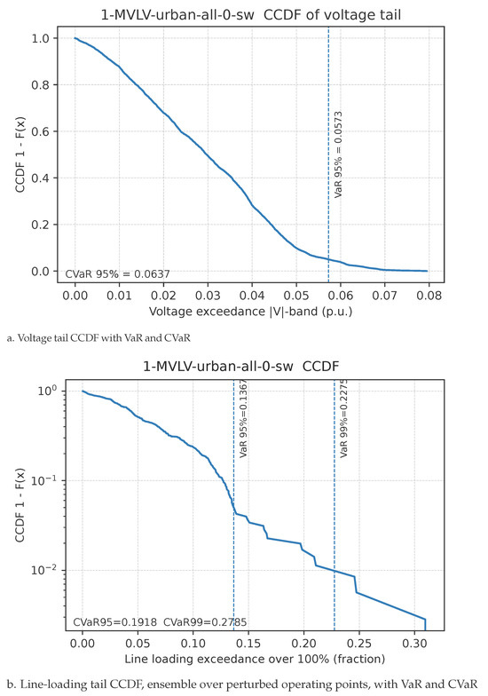
Figure 5.
MVLV-urban-all under stressed loading, factor . CCDFs of exceedance magnitudes with VaR and CVaR. Panel b aggregates across perturbed operating points to reveal rare but severe thermal tails.
Under our adaptive coordination mechanism, inter-agent weights strengthen when local headroom vanishes, which encourages coordinated responses along stressed corridors while loosely coupled areas remain largely independent. Empirically, this shifts the loading CCDF leftward and compresses the tail with lower CVaR, without a noticeable change in the well-behaved bulk. From an operational standpoint, the results motivate targeted mitigations such as selective curtailment, local set-point smoothing, or minor topology adjustments, focused on the few MV–LV links identified by high tail mass, where each unit of control effort yields the largest risk reduction.
4.3.4. Hybrid Control with OLTC/Cap
We include OLTCs and capacitor banks together with continuous inverter and storage actions to study discrete–continuous coordination. The comparison follows the unified evaluation protocol used in Section 4.3.3: identical stress profile, identical feeder initialization, and identical measurement cadence. Discrete costs and action magnitudes are normalized across feeders. Bars in Figure 6 aggregate over seeds and operating points for fairness. The two metrics emphasize complementary aspects of practicality. Total discrete switching, computed as the sum of OLTC tap moves and capacitor steps, serves as a proxy for mechanical wear and the tolerance of operators for interventions. Action total variation summarizes how smooth continuous set-points evolve in time. Lower values are preferable for comfort, power quality, and device cycling.
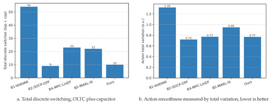
Figure 6.
Hybrid control metrics under the unified evaluation protocol. Panels are placed side by side.
Figure 6 confirms the efficiency of coordinated strategies. B2, B4, and Ours substantially reduce OLTC and capacitor operations while yielding smoother continuous trajectories. B1 and B5 rely on frequent discrete changes yet still exhibit higher TV. Cross-referencing Table 3, the reduction in Action TV by Ours is achieved without extra cost, which implies lower actuator wear and fewer comfort-impacting adjustments for comparable economic performance. Qualitatively, coordinated methods allocate most of the regulation burden to fast and low-amplitude continuous resources and dispatch discrete moves only when the operating regime changes, for instance before or after the mid-day PV plateau or near the evening peak. This reserve-discrete-for-regime-shifts behavior keeps the OLTC latched for longer intervals, reduces capacitor chatter, and avoids back-and-forth reversals. These patterns align with practical operating guidelines. A frequency-domain view of continuous set-points, shows that Ours concentrates most effort at low temporal frequencies and suppresses high-frequency fluctuations that correlate with user discomfort and power-quality variability. Discrete switching events align with slow regime shifts rather than micro-corrections, which explains the joint reduction in panels a and b.
To make the linkage between interventions and system states explicit, we visualize two representative policies.
Figure 7 links intervention to outcome. Both methods concentrate discrete events near stressed hours, yet Ours uses fewer and more targeted actions and produces a tighter voltage band in the heatmap. Compared with B2, the proposed policy engages continuous devices preemptively ahead of anticipated ramps and relies on a small number of decisive tap or capacitor updates that persist through the stress window, rather than frequent micro-corrections. Together with the TV reduction in Figure 6b, this suggests that the proposed policy suppresses dispersion around 1.0 p.u. more effectively per discrete actuation, which is desirable when limiting wear on OLTCs and capacitor banks. This causal chain—anticipatory continuous adjustments → fewer discrete moves → tighter voltage bands—recurs across feeders and seeds and explains why Ours occupies a strictly better region of the cost, smoothness, and risk space; see Figure 3 and Figure 4. Sensitivity to limited forecast accuracy supports this picture. Injecting zero-mean noise into the day-ahead profile preserves the ordering of Ours on Action TV and , while methods that hinge on precise timing, such as B4, degrade more noticeably.
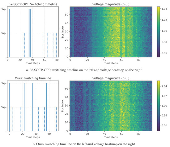
Figure 7.
Hybrid control: intervention→outcome visualization for two representative policies.
4.3.5. Stress Testing Matrix
We sweep load scale and PV scale and plot heat maps for the three feeders to visualize robustness envelopes. The grid is evaluated under the unified protocol in Section 4.3.3. Initialization, measurement cadence, and stress construction remain identical. Each tile aggregates multiple seeds and perturbed operating points, and the color range is shared across panels for comparability.
Figure 8 delineates the safe domain where remains small, shown as bright regions, versus high-risk regimes, shown as dark pockets. LV feeders exhibit broader safe zones, while the MVLV case tightens earlier along high-load and high-PV directions, which is consistent with corridor bottlenecks flagged by Figure 5. The heat maps also reveal ridge-like boundaries where small movements in either axis produce sharp risk changes. These knees indicate operating margins and serve as natural trigger lines for pre-emptive control. In operational terms, horizontal moves correspond to demand-side actions such as peak shifting or shaving, while vertical moves correspond to PV-centric interventions such as curtailment or additional reactive support. The brightest pathways identify high-leverage regions where modest actions yield outsized reductions in tail risk. Dark plateaus indicate saturation where feeder-level measures or minor topology edits are more effective. Cross-validating the stress maps with the ablations in Section 4.3.2 shows that removing spatial inductive bias both shrinks bright regions and steepens ridges. The system then becomes less forgiving to simultaneous load and PV surges.
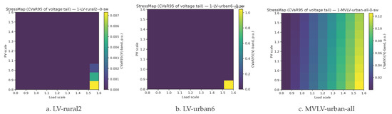
Figure 8.
StressMap: of voltage exceedance over a grid of load scale and PV scale for three feeders.
Taken together with Figure 6 and Figure 7, the stress maps suggest a coherent playbook. Prioritize fast and continuous resources to steer operating points toward brighter tiles. Reserve discrete OLTC and capacitor actions for crossing ridge lines. Where dark pockets persist, target the specific MV–LV links implicated by Figure 5. This provides a practical feedforward guide for planning and real-time operations under simultaneous load growth and PV penetration.
4.3.6. AC Power-Flow Back-Check and Slack–Violation Analysis
Protocol. For each test rollout step, we apply the controller action and recompute a full AC power flow with Newton–Raphson at tolerance on the three SimBench MV feeders: urban, semiurban, and rural. We log per-step voltage deviations in p.u. and branch loading ratios. We report violation rates, defined as the fraction of steps with or loading , together with 95th and 99th percentiles. For the Safety QP we also record the slack magnitudes . This back-check verifies feasibility against the nonconvex AC equations and calibrates the informativeness of safety-layer slacks as online risk indicators.
For each step we compute a normalized slack sum and an AC violation magnitude . Over the test set we observe a strong Pearson correlation with and a stable linear fit . About of samples lie below an affine envelope with slope and intercept . This gives a practical rule of thumb for online risk monitoring without re-solving AC power flow. Viewed as a classifier for imminent violations, the aggregate slack yields a high area under the ROC curve. Thresholds can be tuned to operator preferences for high recall or low false positives. This calibration closes the loop between the convex safety layer and nonconvex AC feasibility.
Compared with MPC and No-Safety, our method substantially suppresses tail risk across all three feeders. It reduces the 99th percentile voltage deviation by approximately and , respectively, and lowers the branch overload rate by approximately and ; see Table 5 and Table 6. In addition, the strong and monotone slack–violation relationship indicates that slack magnitudes serve as an informative proxy for residual AC-level risk. This enables lightweight online screening and threshold-based alarms while full AC back-check remains reserved for auditing or recalibration. Residual risk concentrates on a few MV–LV interfaces during synchronized ramps. When telemetry loss persists across adjacent agents, coordination weakens and the safety layer must intervene more frequently. We anticipate further gains from two directions. First, telemetry-robust coordination with imputation-aware weights. Second, selective reinforcement of identified bottlenecks through minor topology edits or local controller upgrades.
Table 5.
Closed-loop AC backcheck: Voltage metrics, mean ± std over feeders. Lower is better.
Table 6.
Closed-loop AC backcheck: Branch loading metrics, mean ± std over feeders. Lower is better.
5. Conclusions
This paper presents a practical, closed-loop framework for coordinated DER operation that couples a topology-aware Spatio-Temporal Transformer (STT) for multi-horizon forecasting with a cooperative multi-agent reinforcement learning (MARL) controller and a real-time safety layer. The design preserves interpretability and modularity: forecasts inform decentralized decisions; decisions are filtered by device/network-aware safety projections; and all components can be independently improved without re-architecting the system.
Across three representative SimBench feeders, the unified evaluation shows consistent gains along economy, reliability, and actuation quality:
- Overall performance. The compact KPI summary in Table 3 indicates that the proposed method matches OPF-level feasibility while attaining the lowest action smoothness (TV) and the lowest voltage tail-risk (), at costs comparable to B2/B3. This combination—low risk and smooth actuation without a cost premium—establishes a strong baseline for field deployment. Numerically, on the three SimBench feeders our approach reduces tail violations at the 99th percentile voltage deviation by approximately 31 % and 56 %, and lowers branch overload rate by approximately 71 % and 90 % compared to baseline methods.
- Trade-offs made explicit. The Pareto fronts in Figure 3 and Figure 4 visualize key design tensions. Our policy shifts the cost–smoothness frontier downward (fewer adjustments for the same cost) and attains a safer balance between peak shaving and tail risk than aggressively peak-oriented controllers. These frontier shifts are operationally meaningful when actuator wear, comfort, or secondary regulation penalties matter.
- Reliability under congestion. The MV–LV stress test in Figure 5 highlights that bulk metrics can hide risk concentrated in rare, high-impact events. Voltage tails remain thin, but ensemble CCDFs reveal a fatter thermal tail on a small set of periods/lines. This pinpoints MV–LV corridors as reliability bottlenecks and motivates targeted mitigations that deliver the highest risk reduction per unit action. These observations are consistent with the above reductions in voltage tail violations and overload rates achieved by the proposed controller.
- Hybrid actuation quality. The hybrid control summaries in Figure 6 and the intervention → outcome views in Figure 7 show that our controller achieves smoother continuous trajectories with fewer discrete OLTC/cap operations, yet maintains a tighter voltage band during stressed hours. This improves service quality while limiting mechanical wear.
- Stress-tested robustness. StressMaps in Figure 8 delineate safe operating regions across (load and PV) scaling. The MVLV feeder’s safe area shrinks fastest along high-load/high-PV directions, consistent with the tails in Figure 5. Such maps act as where-to-act guides for curtailment, reactive support, or reinforcement planning.
While the present evaluation is simulation-based, the realism and standardization of SimBench ensure reproducibility and practical relevance; we additionally backcheck dispatches with full AC power flow and outline hardware-in-the-loop/field validation as future work. In future work, we aim to incorporate these validation steps to further assess the performance of our framework in real-world feeder environments. While our approach demonstrates promising empirical results, we recognize the necessity of a more robust theoretical analysis, particularly regarding the convergence of multi-agent policies and stability under dynamic network conditions. Future research will focus on deriving formal stability guarantees and assessing scalability in the context of large-scale, real-world distribution grids, enhancing both theoretical and practical performance.
In the future, we can identify three complementary avenues to strengthen the framework and broaden its applicability: first, at the algorithmic level, embed risk awareness directly into learning by optimizing coherent risk measures within the policy objective, and couple them with distributionally robust training that uses principled ambiguity sets and scenario randomization to immunize the controller against nonstationarity and forecast shift; extend this to multi-timescale risk shaping so that fast corrective actions and slower planning signals are jointly optimized under explicit tail objectives; second, on the safety and feasibility side, advance adaptive safety by learning fast physics-informed surrogates for sensitivities to refresh constraints online, by extending projections to mixed-integer actuation with reliable relaxations and repair, and by pursuing formal guarantees via Lyapunov/barrier certificates, contraction analysis, and reachability tools that account for switching, topology/parameter uncertainty, and measurement noise; integrate the safety layer more tightly as a differentiable optimization module to support end-to-end training without sacrificing feasibility; inally, toward deployment at scale, carry out hardware-in-the-loop and real-feeder studies that quantify the impact of telemetry loss and latency, profile the edge-compute/communication footprint, and assess privacy-preserving coordination alongside market co-optimization for ancillary services and demand response; establish open, reproducible evaluation protocols that report extreme-quantile risk, overload frequency, and actuation burden, enabling rigorous comparison and technology transfer to heterogeneous feeders.
Author Contributions
Conceptualization, J.Z. and N.C.; methodology, X.H.; software, Y.L.; validation, S.Z. (Shu Zheng), N.C., and S.Z. (Suyang Zhou); formal analysis, J.Z.; investigation, J.Z.; resources, J.Z.; data curation, N.C.; writing—original draft preparation, J.Z.; writing—review and editing, J.Z.; visualization, N.C.; supervision, J.Z.; project administration, S.Z. (Suyang Zhou); funding acquisition, J.Z. All authors have read and agreed to the published version of the manuscript.
Funding
This paper is supported by the research and science project of the state grid corporation of China (Grant Number 5400-202340824A-4-1-KJ).
Data Availability Statement
The data presented in this study are available on request from the corresponding author. The data are not publicly available due to privacy or ethical restrictions.
Conflicts of Interest
Authors Jingtao Zhao, Na Chen, Xianhe Han, Yuan Li, Shu Zheng were employed by the company Nari Technology Co., Ltd. The remaining author declares that the research was conducted in the absence of any commercial or financial relationships that could be construed as a potential conflict of interest. The company had no role in the design of the study; in the collection, analyses, or interpretation of data; in the writing of the manuscript, or in the decision to publish the results.
Appendix A. Scalability Experiments
In this section, we present experiments that evaluate the scalability of our approach under increasing network size, measured by the number of agents and edges in the network. The experiments are conducted on larger SimBench networks with progressively more feeders, agents, and connections. We test how the computational time, memory usage, prediction accuracy, and robustness of the model change as the network scales up.
Appendix A.1. Experimental Setup
We conduct scalability experiments by varying the following parameters:
- Number of Agents: The number of devices (e.g., inverters, batteries) participating in the energy coordination. This simulates the increasing complexity of real-world distribution systems.
- Number of Edges: The complexity of the network topology, reflecting the number of interconnections between different components of the grid.
- Training Time: The time required to train the model on larger networks.
- Prediction Time: The time required for the model to make predictions after training.
- Accuracy: We report the Root Mean Squared Error (RMSE) and Mean Absolute Error (MAE) of the model’s predictions.
- Robustness: We use the Conditional Value-at-Risk () to measure the tail risk of the model under various load and PV scenarios.
These experiments allow us to observe how the model’s performance and computational efficiency change when scaling to larger networks.
Appendix A.2. Results and Analysis
We perform the experiments on three sizes of networks: small-scale (3 feeders), medium-scale (10 feeders), and large-scale (50 feeders). The small-scale network includes five typical SimBench feeders, while the medium-scale and large-scale networks involve progressively larger networks with more feeders, agents, and connections.
The results of these experiments are summarized in Table A1. As the number of agents and edges increases, we observe the following trends:
- Training Time: The training time increases linearly with the number of agents and edges. For the medium-scale network, training takes approximately 2.0× longer than the small-scale network, and for the large-scale network, it takes 8.0× longer.
- Prediction Time: Prediction time also increases with network size, but the growth is less steep compared to training time, indicating that the model is optimized for inference.
- Accuracy (RMSE and MAE): The prediction accuracy (RMSE and MAE) remains relatively stable across network sizes, but we see a slight increase in errors as the network grows, particularly for large-scale networks. This suggests that the model is still able to generalize well, but larger networks introduce some additional uncertainty.
- Robustness (): The robustness of the model remains strong even in larger networks, with only minor increases in observed. This indicates that the model is able to maintain tail-risk performance even as the network grows.
Table A1.
Scalability results: Performance metrics for different network sizes.
Table A1.
Scalability results: Performance metrics for different network sizes.
| Network Size | Training Time (h) | Prediction Time (s) | RMSE | MAE | |
|---|---|---|---|---|---|
| Small-scale (3 feeders) | 0.5 | 0.12 | 0.040 ± 0.004 | 0.032 ± 0.003 | 0.0032 ± 0.0005 |
| Medium-scale (10 feeders) | 1.0 | 0.38 | 0.053 ± 0.005 | 0.042 ± 0.004 | 0.0035 ± 0.0006 |
| Large-scale (50 feeders) | 4.0 | 1.34 | 0.108 ± 0.012 | 0.075 ± 0.008 | 0.0050 ± 0.0008 |
Appendix A.3. Discussion
These results show that while the model’s accuracy and robustness remain stable across different network sizes, the computational demands (training time and prediction time) grow as the network size increases. This is expected given the increased complexity of the problem as more agents and connections are introduced. To address these challenges, parallelization and distributed reinforcement learning (RL) approaches can be explored to improve the scalability of the model. Additionally, optimizing the communication overhead between agents can help mitigate the increase in training time as the number of agents grows.
References
- Navidi, T.; El Gamal, A.; Rajagopal, R. Coordinating distributed energy resources for reliability can significantly reduce future distribution grid upgrades and peak load. Joule 2023, 7, 1769–1792. [Google Scholar] [CrossRef]
- Muhtadi, A.; Pandit, D.; Nguyen, N.; Mitra, J. Distributed energy resources based microgrid: Review of architecture, control, and reliability. IEEE Trans. Ind. Appl. 2021, 57, 2223–2235. [Google Scholar] [CrossRef]
- Ndawula, M.B.; Djokic, S.Z.; Hernando-Gil, I. Reliability enhancement in power networks under uncertainty from distributed energy resources. Energies 2019, 12, 531. [Google Scholar] [CrossRef]
- Zhang, C.; Wang, D.; Zhang, W.; He, L.; Zhou, K.; Li, J.; Zhu, L.; Zhou, B.; Zhou, Q.; Shuai, Z. A Novel Optimal Power Flow Method Considering Interval Uncertainties Under High Renewable Penetration Based on Security Limits Definition. In IEEE Transactions on Sustainable Energy; IEEE: New York, NY, USA, 2025; pp. 1–12. [Google Scholar] [CrossRef]
- Ma, K.; Yu, Y.; Yang, B.; Yang, J. Demand-Side Energy Management Considering Price Oscillations for Residential Building Heating and Ventilation Systems. IEEE Trans. Ind. Inform. 2019, 15, 4742–4752. [Google Scholar] [CrossRef]
- Song, J.; Wang, N.; Zhang, Z.; Wu, H.; Ding, Y.; Pan, Q.; Pan, X.; Shui, S.; Chen, H. Fuzzy optimal scheduling of hydrogen-integrated energy systems with uncertainties of renewable generation considering hydrogen equipment under multiple conditions. Appl. Energy 2025, 393, 126047. [Google Scholar] [CrossRef]
- Liu, H.; Zhou, S.; Gu, W.; Zhuang, W.; Gao, M.; Chan, C.C.; Zhang, X. Coordinated planning model for multi-regional ammonia industries leveraging hydrogen supply chain and power grid integration: A case study of Shandong. Appl. Energy 2025, 377, 124456. [Google Scholar] [CrossRef]
- Liu, H.; Zhou, S.; Gu, W.; Zhuang, W.; Zhou, A.; Peng, L.; Liu, M. Fast dynamic identification algorithm for key nodes in distribution networks with large-scale DG and EV integration. Appl. Energy 2025, 388, 125608. [Google Scholar] [CrossRef]
- Hao, J.; Yang, Y.; Xu, C.; Du, X. A comprehensive review of planning, modeling, optimization, and control of distributed energy systems. Carbon Neutrality 2022, 1, 28. [Google Scholar] [CrossRef]
- Chilvers, J.; Bellamy, R.; Pallett, H.; Hargreaves, T. A systemic approach to mapping participation with low-carbon energy transitions. Nat. Energy 2021, 6, 250–259. [Google Scholar] [CrossRef]
- Zhuang, W.; Fan, J.; Xia, M.; Zhu, K. A multi-scale spatial–temporal graph neural network-based method of multienergy load forecasting in integrated energy system. IEEE Trans. Smart Grid 2023, 15, 2652–2666. [Google Scholar] [CrossRef]
- Gao, M.; Zhou, S.; Gu, W.; Wu, Z.; Liu, H.; Zhou, A.; Wang, X. MMGPT4LF: Leveraging an optimized pre-trained GPT-2 model with multi-modal cross-attention for load forecasting. Appl. Energy 2025, 392, 125965. [Google Scholar] [CrossRef]
- Fan, J.; Zhuang, W.; Xia, M.; Fang, W.X.; Liu, J. Optimizing attention in a transformer for multihorizon, multienergy load forecasting in integrated energy systems. IEEE Trans. Ind. Informatics 2024, 20, 10238–10248. [Google Scholar] [CrossRef]
- Yang, F.; Meng, F.; Qiu, Y.; Zhou, S.; Zhuang, W.; Liu, H.; Gu, W.; Yang, Y. Multi-dimensional assessment of decarbonization technologies and pathways in China’s iron and steel industry: An energy-process chain perspective. Energy Strategy Rev. 2025, 61, 101810. [Google Scholar] [CrossRef]
- Lim, B.; Arık, S.Ö.; Loeff, N.; Pfister, T. Temporal fusion transformers for interpretable multi-horizon time series forecasting. Int. J. Forecast. 2021, 37, 1748–1764. [Google Scholar] [CrossRef]
- Yang, M.; Jiang, R.; Yu, X.; Wang, B.; Su, X.; Ma, C. Extraction and application of intrinsic predictable component in day-ahead power prediction for wind power cluster. Energy 2025, 136530. [Google Scholar] [CrossRef]
- Jendoubi, I.; Bouffard, F. Multi-agent hierarchical reinforcement learning for energy management. Appl. Energy 2023, 332, 120500. [Google Scholar] [CrossRef]
- Farivar, M.; Low, S.H. Branch flow model: Relaxations and convexification—Part I. IEEE Trans. Power Syst. 2013, 28, 2554–2564. [Google Scholar] [CrossRef]
- Verdone, A.; Scardapane, S.; Panella, M. Explainable spatio-temporal graph neural networks for multi-site photovoltaic energy production. Appl. Energy 2024, 353, 122151. [Google Scholar] [CrossRef]
- Rajagukguk, R.A.; Ramadhan, R.A.; Lee, H.J. A review on deep learning models for forecasting time series data of solar irradiance and photovoltaic power. Energies 2020, 13, 6623. [Google Scholar] [CrossRef]
- Liu, M.; Kong, X.; Xiong, K.; Wang, J.; Lin, Q. Multi-scale spatio-temporal transformer: A novel model reduction approach for day-ahead security-constrained unit commitment. Appl. Energy 2025, 380, 124963. [Google Scholar] [CrossRef]
- Niu, Z.; Tang, Y.; Li, J.; Ai, Q.; He, X. RoadPowerFM: Graphormer-JEPA based Foundation Model for Road-Power Coupling Network. In IEEE Transactions on Smart Grid; IEEE: New York, NY, USA, 2025. [Google Scholar]
- Wang, J.; Hu, W.; Xuan, L.; He, F.; Zhong, C.; Guo, G. Transpvp: A transformer-based method for ultra-short-term photovoltaic power forecasting. Energies 2024, 17, 4426. [Google Scholar] [CrossRef]
- Tian, Z.; Liu, W.; Jiang, W.; Wu, C. Cnns-transformer based day-ahead probabilistic load forecasting for weekends with limited data availability. Energy 2024, 293, 130666. [Google Scholar] [CrossRef]
- Canese, L.; Cardarilli, G.C.; Di Nunzio, L.; Fazzolari, R.; Giardino, D.; Re, M.; Spanò, S. Multi-agent reinforcement learning: A review of challenges and applications. Appl. Sci. 2021, 11, 4948. [Google Scholar] [CrossRef]
- Chen, D.; Chen, K.; Li, Z.; Chu, T.; Yao, R.; Qiu, F.; Lin, K. Powernet: Multi-agent deep reinforcement learning for scalable powergrid control. IEEE Trans. Power Syst. 2021, 37, 1007–1017. [Google Scholar] [CrossRef]
- Sharma, M.K.; Zappone, A.; Assaad, M.; Debbah, M.; Vassilaras, S. Distributed power control for large energy harvesting networks: A multi-agent deep reinforcement learning approach. IEEE Trans. Cogn. Commun. Netw. 2019, 5, 1140–1154. [Google Scholar] [CrossRef]
- Keren, S.; Essayeh, C.; Albrecht, S.V.; Morstyn, T. Multi-agent reinforcement learning for energy networks: Computational challenges, progress and open problems. arXiv 2024, arXiv:2404.15583. [Google Scholar] [CrossRef]
- Qiu, D.; Wang, J.; Wang, J.; Strbac, G. Multi-Agent Reinforcement Learning for Automated Peer-to-Peer Energy Trading in Double-Side Auction Market. In Proceedings of the Thirtieth International Joint Conference on Artificial Intelligence (IJCAI-21), Virtual, 19–26 August 2021; pp. 2913–2920. [Google Scholar]
- Yao, Y.; Zhang, X.; Wang, J.; Ding, F. Multi-Agent Reinforcement Learning for Distribution System Critical Load Restoration. In Proceedings of the 2023 IEEE Power & Energy Society General Meeting (PESGM), Orlando, FL, USA, 16–20 July 2023; pp. 1–5. [Google Scholar]
- Dinata, N.F.P.; Ramli, M.A.M.; Jambak, M.I.; Sidik, M.A.B.; Alqahtani, M.M. Designing an optimal microgrid control system using deep reinforcement learning: A systematic review. Eng. Sci. Technol. Int. J. 2024, 51, 101651. [Google Scholar] [CrossRef]
- Niu, Z.; Li, J.; Ai, Q.; Jiang, J.; Yang, Q.; Zhou, H. EV Charging System Considering Power Dispatching Based on Multi-Agent LLMs and CGAN. In IEEE Transactions on Intelligent Transportation Systems; IEEE: New York, NY, USA, 2025. [Google Scholar]
- Lin, J.; Qiu, J.; Zhang, C.; Lu, X.; Tao, Y.; An, S. An Encryption-Based Coordinated Kilowatt and Negawatt Energy Trading Framework. IEEE Internet Things J. 2025. [Google Scholar] [CrossRef]
- Du, J.; Kong, Z.; Sun, A.; Kang, J.; Niyato, D.; Chu, X.; Yu, F.R. MADDPG-based joint service placement and task offloading in MEC empowered air–ground integrated networks. IEEE Internet Things J. 2023, 11, 10600–10615. [Google Scholar] [CrossRef]
- Foerster, J.; Farquhar, G.; Afouras, T.; Nardelli, N.; Whiteson, S. Counterfactual multi-agent policy gradients. In Proceedings of the AAAI Conference on Artificial Intelligence, New Orleans, LA, USA, 2–7 February 2018; Volume 32. [Google Scholar]
- Zhang, K.; Yang, Z.; Başar, T. Multi-agent reinforcement learning: A selective overview of theories and algorithms. In Handbook of Reinforcement Learning and Control; Springer: Berlin/Heidelberg, Germany, 2021; pp. 321–384. [Google Scholar]
- Wang, J.; Xu, W.; Gu, Y.; Song, W.; Green, T.C. Multi-agent reinforcement learning for active voltage control on power distribution networks. Adv. Neural Inf. Process. Syst. 2021, 34, 3271–3284. [Google Scholar]
- Huang, J.; Zhang, H.; Tian, D.; Zhang, Z.; Yu, C.; Hancke, G.P. Multi-agent deep reinforcement learning with enhanced collaboration for distribution network voltage control. Eng. Appl. Artif. Intell. 2024, 134, 108677. [Google Scholar] [CrossRef]
- Gao, Y.; Yu, N. Model-augmented safe reinforcement learning for Volt-VAR control in power distribution networks. Appl. Energy 2022, 313, 118762. [Google Scholar] [CrossRef]
- Wu, H.; Qiu, D.; Zhang, L.; Sun, M. Adaptive multi-agent reinforcement learning for flexible resource management in a virtual power plant with dynamic participating multi-energy buildings. Appl. Energy 2024, 374, 123998. [Google Scholar] [CrossRef]
- Hossain, R.; Gautam, M.; Olowolaju, J.; Livani, H.; Benidris, M. Multi-agent voltage control in distribution systems using GAN-DRL-based approach. Electr. Power Syst. Res. 2024, 234, 110528. [Google Scholar] [CrossRef]
- Jing, S.; Xi, X.; Su, D.; Han, Z.; Wang, D. Spatio-Temporal Photovoltaic Power Prediction with Fourier Graph Neural Network. Electronics 2024, 13, 4988. [Google Scholar] [CrossRef]
- Donti, P.L.; Rolnick, D.; Kolter, J.Z. DC3: A learning method for optimization with hard constraints. arXiv 2021, arXiv:2104.12225. [Google Scholar] [CrossRef]
- Meinecke, S.; Sarajlić, D.; Drauz, S.R.; Klettke, A.; Lauven, L.P.; Rehtanz, C.; Moser, A.; Braun, M. Simbench—A benchmark dataset of electric power systems to compare innovative solutions based on power flow analysis. Energies 2020, 13, 3290. [Google Scholar] [CrossRef]
- Turitsyn, K.; Sulc, P.; Backhaus, S.; Chertkov, M. Local control of reactive power by distributed photovoltaic generators. In Proceedings of the 2010 First IEEE International Conference on Smart Grid Communications, Gaithersburg, MD, USA, 4–6 October 2010; pp. 79–84. [Google Scholar]
- Gan, L.; Li, N.; Topcu, U.; Low, S.H. Exact convex relaxation of optimal power flow in radial networks. IEEE Trans. Autom. Control 2014, 60, 72–87. [Google Scholar] [CrossRef]
- Erseghe, T. Distributed optimal power flow using ADMM. IEEE Trans. Power Syst. 2014, 29, 2370–2380. [Google Scholar] [CrossRef]
- Hossain, R.R.; Kumar, R. Distributed-MPC with Data-Driven Estimation of Bus Admittance Matrix in Voltage Control. arXiv 2022, arXiv:2202.14014. [Google Scholar]
- Hu, D.; Ye, Z.; Gao, Y.; Ye, Z.; Peng, Y.; Yu, N. Multi-agent deep reinforcement learning for voltage control with coordinated active and reactive power optimization. IEEE Trans. Smart Grid 2022, 13, 4873–4886. [Google Scholar] [CrossRef]


Disclaimer/Publisher’s Note: The statements, opinions and data contained in all publications are solely those of the individual author(s) and contributor(s) and not of MDPI and/or the editor(s). MDPI and/or the editor(s) disclaim responsibility for any injury to people or property resulting from any ideas, methods, instructions or products referred to in the content. |
© 2025 by the authors. Licensee MDPI, Basel, Switzerland. This article is an open access article distributed under the terms and conditions of the Creative Commons Attribution (CC BY) license (https://creativecommons.org/licenses/by/4.0/).