Abstract
In high-voltage direct-current (HVDC) transmission and large-scale power-system operation, DC-bias effects can drive current-transformer (CT) cores into premature saturation, distorting the secondary current and seriously jeopardizing the reliability of protective relaying and metering. To address the limited fitting capability and robustness of conventional compensation approaches in the presence of nonlinear distortion, this paper proposes a convolutional neural network (CNN)-based inversion method for CT saturation current. First, a simulation model is built on the PSCAD/EMTDC platform to generate a dataset of saturated, distorted currents covering DC components from −50 A to +50 A. Then, a CNN with a three-layer one-dimensional convolutional architecture is designed; leveraging local convolutions and parameter sharing, it extracts features from current sequences and reconstructs the true primary current. Simulation results show that the proposed method accurately recovers the primary-current waveform under mild-to-severe saturation, with errors within 2%, and exhibits strong adaptability and robustness with respect to both the polarity and magnitude of the DC component. These findings verify the effectiveness of CNNs for CT-saturation compensation.
1. Introduction
In modern power systems, current transformers (CTs) serve as critical devices for measurement and protection, and they are widely applied in transmission, distribution, and generation stages [1]. Their accuracy directly affects the secure and reliable operation of protective relaying, metering, and control systems. However, in high-voltage direct current (HVDC) transmission and long-distance AC transmission, factors such as monopolar ground-return operation, geomagnetically induced currents (GICs), and non-uniform grounding resistances inevitably introduce DC components into the AC network [2,3]. These components cause DC bias in CT cores, driving them into premature saturation and leading to waveform distortion, ratio errors, and phase deviations, which in turn seriously compromise metering accuracy and protection reliability [4,5].
To mitigate CT distortion under DC bias, a variety of methods have been proposed. Physics-based approaches grounded in ferromagnetic modeling [6,7] can reproduce saturation characteristics but require precise parameter identification and involve heavy computational complexity. Signal-processing methods such as least-squares fitting and harmonic-based analysis [8,9,10] are computationally efficient, yet their accuracy deteriorates significantly under severe saturation or nonstationary conditions. Hardware-based solutions, for example, magnetic-field sensors in the CT air gap [11] or self-powered constant-voltage compensation circuits [12], provide stable performance but demand structural modifications, increased cost, and complex calibration, which restrict their large-scale application. Data-driven approaches, such as artificial neural networks [13] and radial basis function models optimized with the SAGA algorithm [14], exhibit strong potential in handling nonlinear distortions and noisy conditions, but their performance remains heavily dependent on the diversity of training data. Existing datasets are often narrow in coverage, failing to capture the full spectrum from mild to deep saturation, and the weak interpretability of such models further limits their engineering acceptance. Overall, while each method has made valuable contributions, none has yet achieved the required balance of high accuracy, robustness, scalability, and interpretability.
To overcome these limitations, this study proposes a convolutional neural network (CNN)-based inversion method for CT saturation current under DC bias. A dataset covering diverse saturation levels is first constructed using the PSCAD/EMTDC simulation platform to ensure comprehensive representation of practical operating conditions. Based on this dataset, a one-dimensional CNN architecture is designed to retain complete temporal resolution and to extract subtle nonlinear distortion features, leveraging local convolution and parameter sharing to achieve accurate reconstruction of the primary current. Simulation results demonstrate that the proposed method maintains stable compensation performance under different DC-bias magnitudes and noise conditions, delivering significantly higher accuracy compared with traditional physics-based, signal-processing, and shallow-learning approaches. Furthermore, the method exhibits superior robustness and generalization ability, providing a promising technical pathway for reliable CT compensation under DC bias and offering both theoretical significance and engineering value for metering and protection in HVDC and large-scale AC power systems.
2. DC-Bias Mechanism Analysis
2.1. DC-Bias Equivalent Analysis
The circulation path of DC-bias current in an AC system is shown in Figure 1. The neutral points of transformers T1 and T2 are connected to the system ground through grounding resistances R1 and R2, respectively, forming a closed loop. When a DC current Idc is injected into the system, a steady DC conduction path is established along the windings and the grounding network [15].
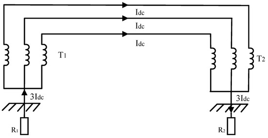
Figure 1.
Circulation Path of DC-Bias Current.
The single-phase equivalent circuit of the CT is driven by an AC source udc together with a superimposed DC current source Idc, acting on the CT winding and the load impedance Z. The single-phase equivalent circuit is shown in Figure 2. In this model, the CT winding is represented by an inductive element; the DC component establishes a constant flux in the core, so that the AC magnetization operates with a DC magnetization offset [16]. When the magnitude of the DC component becomes large, the core enters saturation prematurely, which significantly reduces the equivalent inductance. Consequently, the transfer relationship between the secondary voltage and current is altered, resulting in distortion of the output signal.
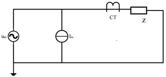
Figure 2.
Single-Phase Equivalent Circuit of the CT.
2.2. Equivalent Model of the CT
The CT equivalent circuit is shown in Figure 3. In the circuit, i1 is the primary-side input current, representing the system primary current; Z1 is the primary-winding impedance—comprising winding resistance and leakage reactance—and reflects primary-side power losses and magnetic-field distribution. The secondary-side output current is i2; Zs denotes the secondary-winding leakage impedance, and ZL is the secondary load impedance. Together they form the secondary loop impedance, which governs the transfer and transformation of the secondary current. The core is represented by the equivalent impedance Ze, which captures the magnetization characteristics of the core—the key component that couple energy and signals between the primary and secondary sides. The magnetizing current ie arises from core hysteresis, eddy currents, and the magnetization requirement, and it affects current-transformation accuracy. The induced electromotive force e in the core serves as the critical link of electromagnetic induction between the primary and secondary, driving the secondary current and maintaining electromagnetic balance [17].
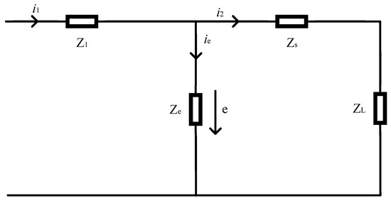
Figure 3.
Equivalent Circuit Diagram of the CT.
2.3. Mechanism of DC-Bias Effects on CT
As shown in Figure 4, when the primary current contains a DC component, the core-flux waveform is offset under superposed AC–DC excitation. In the absence of DC, curve (a) is symmetric about zero. With DC, curve (b) is shifted by the superimposed DC flux, driving the half cycle aligned with the DC polarity toward the saturation knee and reducing its headroom, while the opposite half cycle experiences a corresponding relief. This asymmetry is reflected in the magnetizing current: as in curve (c), a DC component appears together with half-wave distortion and sharp peaks. Fundamentally, DC bias induces a flux-walk phenomenon; as the cumulative flux approaches the saturation limit, the core enters unilateral saturation, causing a rapid increase and severe distortion of the magnetizing current. The ensuing clipping and deformation of the secondary current inflate ratio and phase errors and introduce substantial harmonic content—particularly even-order components arising from half-wave asymmetry—thereby compromising CT metering accuracy and the reliability of protection schemes.
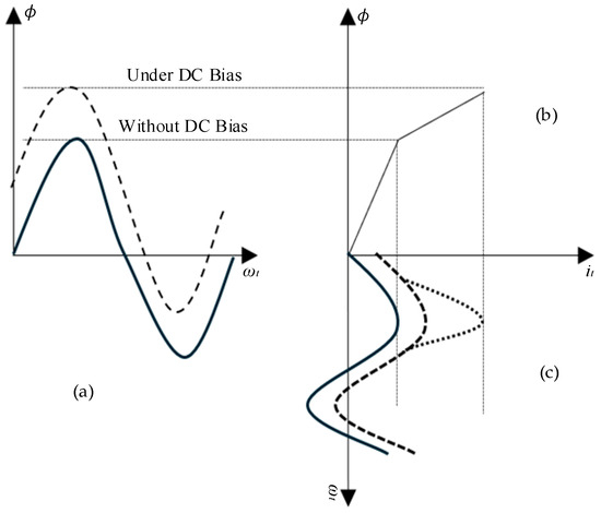
Figure 4.
Schematic of the DC-Bias Mechanism.
3. CT Saturation Detection
The Fourier Transform (FT) is a fundamental tool in signal processing. Its central premise is that any periodic or aperiodic signal can be represented as a superposition of sine and cosine functions. The FT not only reveals a signal’s frequency composition but also provides amplitude and phase information, thereby furnishing the basis for frequency-domain analysis.
For a continuous-time signal x(t), the FT is defined as
where X(f) denotes the complex-valued frequency-domain representation, |X(f)| characterizes the spectral amplitude at each frequency, and ∠X(f) encodes the phase. The inverse Fourier transform reconstructs the time-domain signal:
For a discretely sampled signal x[n], the discrete Fourier transform (DFT) is defined as follows:
while the DFT characterizes the frequency content of discrete signals exactly, its direct computation has a complexity of O(N2). To alleviate the heavy computational load and low efficiency, the fast Fourier transform (FFT) exploits symmetry and periodicity to recursively decompose an N-point DFT into smaller sub-DFTs, thereby reducing the complexity to O(Nlog2N) and significantly accelerating frequency-domain analysis.
The hallmark of CT saturation is distortion of the secondary current waveform arising from asymmetric core saturation, yielding a mixed signal composed of the sinusoidal fundamental together with odd- and even-order harmonics. The key advantage of the FFT is that it converts time-domain waveform distortion into quantitative frequency-domain features—harmonic amplitudes and phases—thereby enabling a mapping from harmonic content to saturation severity. Figure 5 presents the harmonic spectra under different magnitudes of the DC component. As shown, although the fundamental peak fluctuates, it remains the dominant component, indicating that the fundamental still governs the CT secondary current even when saturation occurs. As the DC component increases, the magnitudes of the non-fundamental harmonics rise and certain harmonic peaks become more pronounced. This is because stronger DC bias more readily drives the CT into saturation; the core’s nonlinear magnetization produces additional harmonics. The deeper the saturation, the more severe the harmonic distortion, with richer harmonic content and larger harmonic amplitudes.
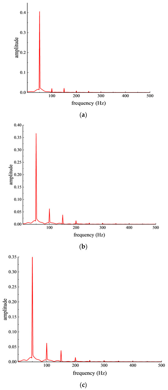
Figure 5.
Amplitude–Frequency Spectra of the Secondary Current under Different DC-Component Magnitudes. (a) Amplitude–Frequency Plot of the Secondary Current at 2 A. (b) Amplitude–Frequency Plot of the Secondary Current at 25 A. (c) Amplitude–Frequency Plot of the Secondary Current at 40 A.
4. CNN-Based Saturation-Current Inversion Method
4.1. Network Architecture and Dataset Construction
A convolutional neural network (CNN) is a deep learning architecture inspired by the structure of the biological visual cortex. Its core advantage lies in using local convolutions and parameter sharing to efficiently extract local features from time-series data while reducing the number of trainable parameters. For the CT saturation-current inversion task in this study, a one-dimensional (1D) CNN is implemented using the MATLAB Deep Learning Toolbox. The core architecture comprises a sequence input layer, 1D convolutional layers, activation layers, a fully connected layer, and a regression output layer [18].
The sequence input layer serves as the model’s input interface and must match the dimensional characteristics of the CT current signal. The 1D convolutional block employs three 1D convolutional layers for feature extraction. All kernels have size 5 × 1, and the padding mode is set to “same” to avoid losing edge information. The numbers of filters are 64, 128, and 256 for the three layers, enabling a progression from low-level local features to higher-level distortion features. The layer wise operation follows the standard formulation, expressed as follows:
where the kernel length is K = 5; wl(k) denotes the weight of the l-th layer’s convolutional kernel; and xl−1(i−k) denotes the (i−k)-th sample of the input current sequence.
In the proposed network architecture, each one-dimensional convolutional layer is immediately followed by a ReLU (Rectified Linear Unit) activation function, expressed as y = max (0, x). This nonlinear transformation plays a central role in enhancing the network’s ability to capture the complex distortion patterns of CT signals under DC-bias conditions. By suppressing negative values while retaining positive responses, ReLU increases the sparsity of feature representations, allowing the network to focus more effectively on salient waveform characteristics. At the same time, it mitigates the vanishing-gradient problem that often hampers the training of deep networks, ensuring stable gradient propagation across layers and accelerating convergence.
Unlike conventional convolutional neural networks, this architecture deliberately omits pooling layers. Although pooling is widely adopted in image and speech recognition tasks to reduce dimensionality and improve translation invariance, it inevitably discards fine-grained temporal details. In the context of primary-current reconstruction, where each sampling point may contain critical information about saturation-induced distortions, such loss of detail would significantly undermine performance. To preserve the complete temporal resolution, the features extracted from the three successive 1D convolutional layers are fed directly into a fully connected layer, which performs a linear projection to a vector whose length matches the number of input time steps. This design enforces a strict one-to-one correspondence between the input and output sequences.
Finally, a regression head produces the reconstructed primary-current waveform by mapping the projected feature vector back to the time domain. In this way, the model implements an end-to-end inversion process, transforming distorted secondary-current measurements into accurate primary-current estimates. This architecture not only provides strong nonlinear modeling and feature extraction capabilities but also retains critical temporal information, thereby laying a solid methodological foundation for high-precision current estimation. For transparency and reproducibility, the principal hyperparameters of the CNN—such as the number of convolutional layers, kernel size, filter counts, learning rate, and training epochs—are summarized in Table 1. These values were selected to balance accuracy and efficiency: three convolutional layers provide sufficient depth without excessive complexity; a kernel size of 5 preserves fine temporal details while capturing distortion patterns; the progressive filter numbers (64/128/256) enhance feature extraction across levels; 200 training epochs ensure convergence; and a learning rate of 0.0005 yields stable yet effective optimization.

Table 1.
CNN Model Hyperparameters.
To ensure clarity and reproducibility, the dataset used in this study is defined as follows. Each sample consists of a pair (x, y), where x denotes the secondary current sequence measured under a specific DC-bias condition and y represents the corresponding rated primary current. The secondary current is converteds to the primary side using the CT transformation ratio, ensuring that both input and output share the same physical unit (amperes). A controllable DC source is connected to the transformer neutral to inject a DC component into the CT primary, with the bias magnitude ranging from −50 A to +50 A, thereby covering typical operating conditions in high-voltage substations. To guarantee sample continuity and resolution, the DC step size is set to 0.2 A, yielding a total of 501 distinct operating points. For each operating point, current sequences are generated on the PSCAD/EMTDC platform using the Jiles–Atherton core model, which captures nonlinear magnetization, remanence, and eddy-current effects, and both steady-state and transient segments are included. In this way, the dataset comprehensively represents light to severe saturation states and provides consistent, physically meaningful supervisory signals for CNN training.
Furthermore, the CT core is modeled in PSCAD/EMTDC using the Jiles–Atherton hysteresis model, which provides a realistic representation of nonlinear magnetization, remanence, and eddy-current effects. The simulation is executed with a sampling frequency of 8 kHz and a total time span of 0.5 s per case, ensuring that both transient and steady-state characteristics are captured. To further improve the robustness of the dataset, Gaussian white noise with varying signal-to-noise ratios (SNRs) is superimposed onto the secondary current, enabling the trained model to generalize under practical measurement conditions where sensor noise and electromagnetic interference are inevitable. After dataset generation, the samples are randomly divided into training and validation sets with a ratio of 8:2, ensuring sufficient data for model learning while preserving an independent subset for unbiased performance evaluation. This strategy not only spans the full DC-bias range but also incorporates diverse noise levels, thereby strengthening the network’s ability to handle real-world CT distortion scenarios.
To quantify the CNN’s inversion error for CT saturation current, the following formulas are adopted [19]:
where I1 denotes the RMS value of the theoretical current, and I0 denotes the RMS value of the compensated current.
4.2. Model Interpretability Analysis
To further interpret the learned representations, the frequency responses and dominant sensitive frequencies of the first convolutional layer were analyzed.
As shown in Figure 6, most filters exhibit strong responses in the low-frequency region (normalized frequency below 0.2), corresponding to the DC component and even-order harmonics induced by core saturation. A smaller number of filters respond to higher frequencies, reflecting sensitivity to waveform clipping and recovery edges.
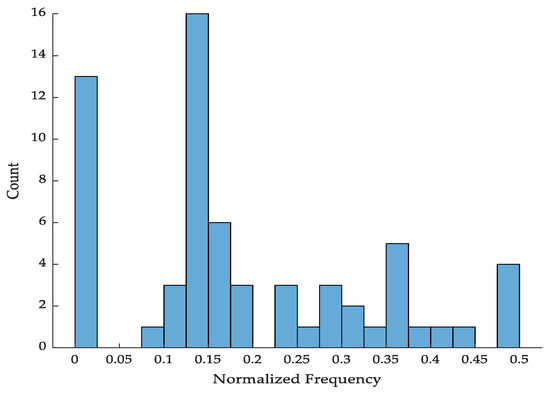
Figure 6.
Distribution of Main Sensitive Frequencies of conv1 Filters.
The histogram of main sensitive frequencies (Figure 7) further confirms that the CNN primarily captures low-frequency bias and nonlinear harmonic features, consistent with the physical mechanism of DC-biased CT saturation.
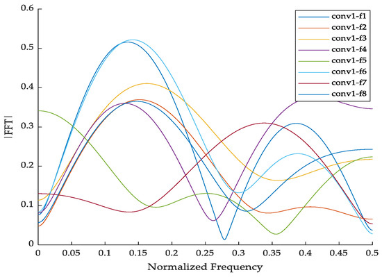
Figure 7.
Amplitude–Frequency Responses of conv1 Filters.
These results demonstrate that the proposed CNN not only achieves accurate numerical inversion but also learns features that align with the underlying electromagnetic phenomena.
5. Simulation Validation
5.1. Establishment of the Simulation Model
To faithfully reproduce the saturation characteristics of a CT under DC bias, a simulation model was implemented in PSCAD/EMTDC, which provides microsecond-level dynamic-response capability. The model schematic is shown in Figure 8. DC bias is emulated by connecting a DC source to the transformer neutral. The CT is represented using PSCAD’s built-in Jiles–Atherton (J–A) hysteresis model. The sampling frequency is 8 kHz and the total simulation time is 0.5 s. The J–A model parameters are listed in Table 2.
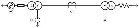
Figure 8.
PSCAD/EMTDC simulation model for CT saturation.
Table 2.
Jiles–Atherton model parameters for CT simulation.
5.2. Simulation Results
The data generated by the simulation model were used as inputs to the CNN, and the resulting compensated (reconstructed primary-current) waveform is shown in Figure 9, illustrated for a DC component of 35.4 A.
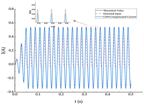
Figure 9.
Comparison of true, distorted, and CNN-reconstructed current (DC = 35.4 A).
In the figure, the black solid line denotes the true primary-current waveform—the ideal signal a CT should reproduce—and serves as the target for CNN inversion. The red dashed line denotes the CT secondary current under DC bias/saturation, showing pronounced distortion over the initial portion of the waveform. The blue solid line denotes the CNN-reconstructed current, which is nearly coincident with the black curve; deviations in the steady-state segment are negligible. This demonstrates that the CNN successfully recovers the original characteristics of the distorted waveform.
To substantiate the CNN’s compensation performance for CT saturation current, ten representative DC-bias operating cases were selected from the simulation dataset for targeted validation. The error was computed according to (5), and the detailed results are reported in Table 3.
Table 3.
CNN validation results under representative DC-bias conditions.
Table 3 shows that the error in all operating cases is below 2%, indicating that the CNN maintains strong compensation performance across different DC-component levels. Rather than varying monotonically with the bias magnitude, the error reflects the inherently nonlinear effect of DC bias on CT core saturation, where the magnetization curve undergoes stage-wise transitions instead of linear compression as the bias increases, making the severity of saturation not strictly proportional to the bias amplitude. As a result, the inversion error exhibits a stable yet non-monotonic profile, while the CNN, by reconstructing the primary current from the overall distorted waveform rather than relying solely on the DC component magnitude, achieves consistently high accuracy even under extreme conditions, with only slight increases that remain within acceptable limits.
5.3. Dataset Partitioning and Cross-Validation
To avoid overfitting and to evaluate the robustness of the proposed model, the dataset was randomly divided into training and validation sets with a ratio of 8:2, ensuring that sufficient data were available for model learning while preserving an independent subset for unbiased performance evaluation. Furthermore, a 5-fold cross-validation scheme was conducted to comprehensively examine the model’s stability. Specifically, the dataset was partitioned into five mutually exclusive subsets, with each subset used once as the test set and the remaining four as the training set. This process was repeated five times so that every sample was included in the testing stage. For each fold, RMSE and MAE were computed, and their mean and standard deviation were reported as overall performance indicators. As shown in Figure 10, the errors exhibit small variations across different folds, with RMSE = 0.0016 ± 0.0006 and MAE = 0.0014 ± 0.0005, demonstrating the strong generalization ability and robustness of the proposed method.
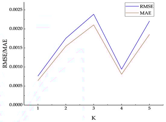
Figure 10.
RMSE and MAE results under 5-fold cross-validation.
5.4. Influence of Noise
In practical applications, current signals are unavoidably contaminated by noise; hence, assessing the model’s robustness across different signal-to-noise ratio (SNR) conditions is essential. In this study, we superimposed zero-mean Gaussian white noise with controlled variance onto the distorted input current and evaluated performance at each SNR using RMSE and the coefficient of determination (R2). As shown in Figure 11 and Figure 12, RMSE decreases markedly while R2 rises monotonically as SNR increases. When SNR is below 20 dB, both metrics show modest fluctuations that remain within acceptable bounds; once SNR reaches 30 dB and above, the curves stabilize—RMSE stays low and R2 approaches a plateau—indicating reliable reconstruction of the primary current. Relative to the noiseless baseline, the model maintains acceptable accuracy even under low-SNR conditions, demonstrating intrinsic robustness to measurement noise.
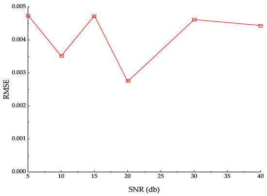
Figure 11.
Effect of Different SNRs on RMSE.
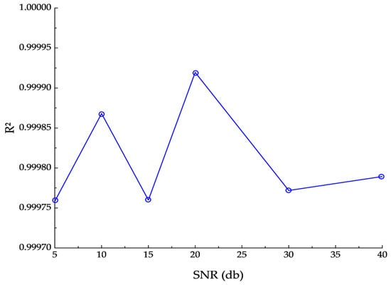
Figure 12.
Effect of Different SNRs on R2.
Overall, the CNN model can achieve near-ideal reconstruction performance when the SNR is relatively high. Although the errors increase under stronger noise, the variations remain within an acceptable range. This suggests that the proposed approach has strong practical potential, ensuring reliable estimation results even when measurement signals are contaminated by unavoidable noise.
5.5. Comparative Analysis with Other Methods
To further evaluate the performance of the proposed CNN-based inversion method, its results were compared with those obtained from two other commonly used approaches: gated recurrent unit (GRU) networks and radial basis function (RBF) neural networks. The comparison was conducted in terms of RMSE and MAE, and the results are summarized in Table 4.
Table 4.
Performance comparison of CNN, GRU, and RBF methods in terms of RMSE and MAE.
As shown in Table 4, the CNN, CNN–GRU, and attention-based models all achieve sub-milli per-level inversion errors, demonstrating strong capability in reconstructing the primary current under DC-bias conditions. The baseline CNN attains an RMSE of 0.00087 and an MAE of 0.00077, while the hybrid CNN–GRU model achieves slightly lower values of 0.00076 and 0.00071, respectively. The attention-based model also performs competitively, with an RMSE of 0.00094 and an MAE of 0.00089. These results indicate that incorporating temporal-dependency modeling or attention weighting provides marginal accuracy improvements under certain noise conditions, but the overall gains are limited, whereas the computational cost increases substantially.
The RBF network achieves an RMSE of 0.00116 and an MAE of 0.00083, yielding results that are close to those of the CNN despite its simpler structure. This can be attributed to the RBF’s inherent ability for local nonlinear fitting and the relatively smooth statistical characteristics of CT current waveforms under controlled DC-bias excitation. In such low-dimensional mapping scenarios, the RBF can approximate the input–output relationship effectively. However, as saturation deepens or noise levels increase, the RBF model exhibits a more pronounced decline in generalization and stability compared with the CNN.
Overall, the comparative results verify the rationality of the proposed CNN design. The CNN provides an optimal balance among accuracy, robustness, and computational efficiency, outperforming both traditional shallow-learning methods and more complex hybrid architectures. While CNN–GRU and attention-based variants show potential for incremental improvements, the baseline CNN remains the most practical and efficient choice for real-time CT saturation-compensation applications due to its lightweight structure and consistent performance across diverse operating conditions.
6. Conclusions
This study explored the influence of DC bias on current transformers (CTs) and proposed a CNN-based inversion method to accurately reconstruct primary current. Through theoretical analysis, simulation validation, and extended experiments, several key findings have been obtained.
- (1)
- DC bias shifts the flux trajectory, leading to unilateral core saturation. This results in waveform distortion, magnitude offsets, and increased harmonic content, which compromise the accuracy of metering and the reliability of protective relaying.
- (2)
- By leveraging FFT feature extraction and CNN learning, the proposed method successfully reconstructs distorted signals with high accuracy. Simulation results confirm that errors remain within engineering tolerances under different DC-bias magnitudes.
- (3)
- The model maintains stable performance under different signal-to-noise ratios. Even in low-SNR conditions, RMSE and MAE remain within acceptable limits, showing the method’s strong resistance to measurement noise.
- (4)
- Compared with GRU, RBF, CNN–GRU, and attention-based models, the proposed CNN achieves the best trade-off between accuracy and efficiency. Although hybrid variants offer slight improvements, their higher complexity limits practical benefits. The results confirm the CNN’s strong capability to capture nonlinear distortions under DC-bias conditions.
It should be acknowledged that the present study is based on PSCAD/EMTDC simulations, which ensured a wide coverage of operating conditions and noise scenarios. Nevertheless, validation with real CT measurements has not yet been carried out. Moreover, the current robustness evaluation only considers Gaussian noise. In practical power systems, current signals are often affected by harmonic distortion, flicker, and transient disturbances induced by HVDC operation. Future work will therefore extend this research to hardware experiments and incorporate these realistic disturbance types, providing further evidence of the method’s practical applicability, generalization capability, and robustness.
Author Contributions
Conceptualization: Z.R., K.Y., G.C., Y.Y., Y.C. and L.Z.; Software: Z.R., K.Y., G.C., Y.Y., Y.C. and L.Z.; Writing—original draft preparation: Z.R., K.Y., G.C., Y.Y., Y.C. and L.Z. All authors have read and agreed to the published version of the manuscript.
Funding
This research received no external funding.
Data Availability Statement
The original contributions presented in this study are included in the article. Further inquiries can be directed to the corresponding author.
Conflicts of Interest
Authors Zhanyi Ren, Kanyuan Yu, Yunxiao Yang were employed by the Yangjiang Nuclear Power Co., Ltd. Author Guangbo Chen was employed by the C-EPRI Electric Power Engineering Co., Ltd. The remaining authors declare that the research was conducted in the absence of any commercial or financial relationships that could be construed as a potential conflict of interest.
References
- Huang, Z.; Lin, X.; Ma, X.; Wu, Q.; Wei, F. Reconstruction Method of Saturation Current of Current Transformer in Relay Protection Application Related to Wind Power. Trans. China Electrotech. Soc. 2022, 37, 4823–4834. [Google Scholar] [CrossRef]
- Lin, L. Research on issues related to DC bias. Electr. Eng. Technol. 2021, 129–130, 144. [Google Scholar] [CrossRef]
- Alderete, L.; Tavares, M.C.; Magrin, F. Hardware implementation and real time performance evaluation of current transformer saturation detection and compensation algorithms. Electr. Power Syst. Res. 2021, 196, 107288. [Google Scholar] [CrossRef]
- Huang, T.; Li, Z.; Huang, Q.; Xu, M.; Liu, W. Error calculation method and characteristic analysis of low-voltage metering current transformers under DC bias. Power Syst. Technol. 2025, 49, 373–380. [Google Scholar] [CrossRef]
- Yan, Q.; Li, S.; Ye, Y.; Xiong, R.; Zhao, W. Analysis of measurement characteristics of current transformers under DC bias. Electr. Meas. Instrum. 2021, 58, 144–148. [Google Scholar] [CrossRef]
- Li, J.; Huang, J.; Zhang, Y.; Lin, X.; Zheng, Q. DC compensation method for suppressing current-transformer saturation caused by DC bias. Sci. Technol. Eng. 2021, 21, 3618–3625. [Google Scholar]
- Guo, Z.; Chen, F.; Wu, W.; Liu, J.; Ma, X. Design of a magnetic-balance current transformer based on dynamic reactive compensation. Trans. China Electrotech. Soc. 2022, 37, 217–224. [Google Scholar] [CrossRef]
- Christian, L.; Sergio, T.; Michele, Z. A Simple Method for Compensating Harmonic Distortion in Current Transformers: Experimental Validation. Sensors 2021, 21, 2907. [Google Scholar] [CrossRef] [PubMed]
- Hu, H.; Cui, C.; Yuan, P.; Duan, Y.; Zhang, X. Current-transformer saturation detection and distorted-current compensation. J. Northwest Univ. (Nat. Sci. Ed.) 2022, 52, 52–59. [Google Scholar] [CrossRef]
- Hu, C.; Zhang, Z.; Chen, G.; Li, M.; Yang, A.; Li, D. Online compensation technology for metering current transformers under DC bias. Instrum. Tech. Sens. 2021, 2021, 40–44. [Google Scholar]
- Zhang, Z.; Chen, B.; Wu, Y.; Liu, Z.; Tian, C.; Chen, Y. DC-immunity characteristics of magneto-valve current transformers. Electr. Power Autom. Equip. 2022, 42, 129–135. [Google Scholar] [CrossRef]
- Guo, J.; Yuan, J.; Xie, J.; Lu, S.; Sun, M.; Su, D.; Pan, G.; Jin, L. Constant-voltage parallel current compensation method based on self-powered electromagnetic induction. Sci. Technol. Eng. 2021, 21, 6718–6724. [Google Scholar] [CrossRef]
- Mwongela, E.M.; Koo, C.C. ANN Based Model for Current Transformers’ Saturation Error Compensation in Medium Voltage Switchgears. J. Electr. Eng. Technol. 2022, 17, 2171–2179. [Google Scholar] [CrossRef]
- Wang, B.; Ying, S.; Xiao, Y.; Hu, S.; Fan, X.; Pan, S.; Wang, B. Distorted-current inversion for CTs under DC bias based on RFC–SAGA–RBF. South. Power Syst. Technol. 2024, 18, 51–61. [Google Scholar] [CrossRef]
- Ni, Y.; Yu, K.; Zeng, X.; Len, Y.; Peng, P.; Zhou, W.; Xie, Y. Correlation analysis of transformer DC-bias current caused by metro stray currents. J. Electr. Power Sci. Technol. 2021, 36, 136–143. [Google Scholar] [CrossRef]
- Wu, Y.; Tian, C.; Wu, F.; Chen, Y.; Chen, B. Magneto-valve electromagnetic current transformer. High Volt. Technol. 2020, 46, 3154–3163. [Google Scholar] [CrossRef]
- Lu, S.; Yang, S.; Cai, J.; Zhou, G.; Xu, M. Mechanism of DC-bias effects on current transformers. Electr. Meas. Instrum. 2014, 51, 6–11. [Google Scholar] [CrossRef]
- Yao, C.; Yang, P.; Liu, Z. Load-forecasting method based on a CNN–GRU hybrid neural network. Power Syst. Technol. 2020, 44, 3416–3424. [Google Scholar] [CrossRef]
- Zhang, W.; Xu, L.; Chen, X.; Guo, P.; Li, H.; Zhu, C. Study on error-measurement methods for transformer bushing current transformers. Transforme 2020, 57, 7–11+37. [Google Scholar] [CrossRef]
Disclaimer/Publisher’s Note: The statements, opinions and data contained in all publications are solely those of the individual author(s) and contributor(s) and not of MDPI and/or the editor(s). MDPI and/or the editor(s) disclaim responsibility for any injury to people or property resulting from any ideas, methods, instructions or products referred to in the content. |
© 2025 by the authors. Licensee MDPI, Basel, Switzerland. This article is an open access article distributed under the terms and conditions of the Creative Commons Attribution (CC BY) license (https://creativecommons.org/licenses/by/4.0/).