Spatiotemporal Modeling of Dissolved Oxygen in a Semi-Enclosed Water Body with a LSTM-GRU Hybrid Approach

Abstract

The dynamic evolution of dissolved oxygen (DO) concentration is critical for aquatic ecosystem stability and biodiversity, serving as an important water quality indicator. Predicting DO distribution is challenging due to complex hydrodynamic conditions and environmental disturbances. While traditional experimental methods provide accurate short-term data, they are limited in spatial coverage, costly, and lack real-time predictive capabilities. Computational fluid dynamics (CFD) simulations, though beneficial for mechanism modeling, suffer from high computational costs and reduced accuracy in long-term, nonlinear predictions. This study addresses these limitations by developing an LSTM-GRU Hybrid Model for predicting DO concentration in Shenzhen Bay. Combining Long Short-Term Memory (LSTM) and Gated Recurrent Units (GRU), the model enhances time-memory capabilities and parameter efficiency. Results show that the LSTM-GRU Hybrid Model outperforms single neural networks with a correlation coefficient close to 0.99 and RMSE below 0.04 gO₂/m³. This study not only introduces a novel methodology for modeling dissolved oxygen in Shenzhen Bay, but also contributes to advancing predictive capabilities in earth systems environment and offers methodological insights applicable to similar semi-enclosed marine environments.

1. Introduction

As global water environmental pollution intensifies, water quality monitoring and prediction have become key research areas in environmental science and urban management [1]. This study focuses on the efficient simulation and prediction of the spatial and temporal distribution of dissolved oxygen (DO) concentration, a key indicator in typical urban water bodies such as bays. In semi-enclosed water bodies, DO concentration is influenced by a variety of interacting factors, including tidal exchange, freshwater runoff, water temperature, salinity stratification, and anthropogenic impacts such as domestic sewage discharge, nutrient (nitrogen and phosphorus) loading, and chemical oxygen demand (COD) emissions. These combined natural and human-induced effects result in strong spatiotemporal nonlinearity in DO variation, making accurate prediction particularly challenging [2]. Traditional water quality monitoring mainly relies on field sampling and laboratory analysis. Although the data are reliable, this method is time-consuming, costly, and not suitable for large-scale, high-precision monitoring. To address this issue, computational fluid dynamics (CFD) methods have been introduced to predict DO distribution and provide a detailed description of physical processes. However, CFD methods depend heavily on boundary conditions and initial parameters, are inefficient in high-resolution long-term simulations, and are difficult to meet the practical needs for rapid prediction and response.

In recent years, artificial intelligence technology has rapidly developed, and machine learning, an algorithmic framework capable of automatically learning patterns from data and making predictions, has been widely applied in environmental science, weather forecasting, hydrological simulation, and other fields [3,4,5]. Among these, deep learning, an important branch of machine learning, has demonstrated outstanding performance in time-series prediction and spatiotemporal feature extraction tasks due to its multi-layer neural network structure and powerful feature extraction capabilities. Deep learning offers a potential technological pathway for the efficient simulation of water quality parameters and is expected to break through the bottleneck of traditional methods in terms of efficiency and accuracy, enabling efficient simulation and prediction of DO concentration distribution [6].

Traditional experimental methods have accumulated significant achievements in DO concentration detection. D’Autilia et al. [7] captured short-term oscillation patterns of DO using local maximum time distance analysis. Dubuc et al. [8] and Hishe et al. [9], respectively, used multi-parameter probes to measure dissolved oxygen concentrations in urbanized wetlands and rivers. Beadle [10] improved the Winkler method to estimate oxygen content in polluted waters effectively. Wilkin et al. [11] compared colorimetric, electrode, and modified Winkler titration methods and confirmed the latter’s high-precision advantage under strict data requirements. In addition, Wittkampf et al. [12] developed silicon thin-film sensors, Li et al. [13] introduced luminescent oxygen quenching sensors, and Hydes et al. [14] utilized Optode sensors, all of which demonstrated good stability and linear response characteristics. These methods are accurate and have a solid theoretical foundation; however, they rely on point measurements, making it difficult to comprehensively reflect the spatiotemporal distribution characteristics of complex water bodies. Moreover, high-precision instruments are complex to operate and costly.

Numerical simulation methods expand the spatiotemporal dimension of DO dynamics by coupling environmental factors with physical equations. Abbaspour et al. [15] simulated watershed hydrology and material transport using the SWAT program. Almeida et al. [16] conducted a 19-year long-term water quality simulation of a shallow eutrophic lagoon using the SWAT and CE-QUAL-W2 models. Hull et al. [17] and Antonopoulos et al. [18] used continuous models and one-dimensional layered models to analyze the effects of variables such as water temperature and radiation on DO. Fang et al. [19] used the minlake96 model, and Stefan et al. [20] used vertical transport equations to quantify the correlation between climate and water quality. Carlsson et al. [21] and Chapelle et al. [22] used ecological models to reveal seasonal variations in oxygen concentration and nitrogen–oxygen flux mechanisms. Mandal et al. [23] and Park et al. [24] modeled the diurnal effects of wind speed, light, and aquatic plants using differential equations and the MACRIV model. Hoque et al. [25] proposed the COPSTZ model, focusing on the impact of reduced dissolved oxygen on plankton. In addition, Curbani et al. [26] used CFD to evaluate the dissolved oxygen balance and control processes in the Vitória Island estuarine system in Brazil, and Piehl et al. [27] employed the MOM-ERGOM model to investigate the spatiotemporal variations in seasonal hypoxia and assess oxygen indicators in the western Baltic Sea. Numerical simulation can characterize multi-factor coupling mechanisms, but they depend on precise parameterization and high computational resources and have limited ability to express complex nonlinear relationships.

Machine learning methods break through the limitations of traditional physical frameworks through data-driven modeling. Kisi et al. [28] showed that Bayesian model averaging (BMA) outperforms traditional statistical models in DO prediction. Ahmed [29] and Zare Abyaneh [30] verified the strong fitting ability of ANN for biochemical indicators. Ramaraj and Sivakumar [31] compared the performance of ANFIS, LSTM, and NAR neural networks in water quality prediction. Elkiran et al. [32] and Ay et al. [33] confirmed the robustness of the ANFIS and RBNN models in multi-step predictions, while Faruk [34] improved time-series prediction accuracy using an ARIMA-neural network hybrid framework. However, existing research mainly focuses on single models, with certain limitations in capturing the spatiotemporal dynamics of DO under tidal influences.

Based on the above analysis, this paper proposes a hybrid deep learning model combining Long Short-Term Memory (LSTM) networks and Gated Recurrent Units (GRU) for predicting the spatiotemporal distribution of DO concentration in Shenzhen Bay. Compared with single models used in existing studies, the LSTM-GRU Hybrid Model demonstrates distinct advantages both theoretically and practically. From a theoretical perspective, the model leverages the strengths of LSTM in modeling long-term dependencies in time series and the computational efficiency of GRU, thereby overcoming the traditional trade-off between prediction accuracy and computational cost. From a practical perspective, comparative experiments with LSTM, Multilayer Perceptron (MLP), K-Nearest Neighbors (KNN), and Recurrent Neural Network (RNN) models confirm its applicability under complex hydrological conditions, offering a feasible solution to meet the dual requirements of real-time performance and accuracy in water quality prediction for bay areas. This study not only deepens the understanding of deep learning mechanisms in predicting complex water bodies but also provides an efficient, intelligent, data-driven predictive tool for coastal ecological environment management.

This study uses Shenzhen Bay as a typical research area. As an important nearshore area of the Pearl River Estuary, Shenzhen Bay is influenced by urban development, pollution pressure, and marine ecological changes. Its water quality directly affects the health of the ecosystem and regional sustainable development. Additionally, the bay’s strong tidal dynamics and frequent human interference present complex hydrodynamic structures, making it a typical and challenging testing ground for deep learning algorithms. This study not only provides a technical solution for ecological early warning in coastal areas but also helps validate the ability of deep learning models to handle complex environmental system data, contributing to the theoretical refinement and methodological innovation of deep learning in environmental science.

2. Methodology

2.1. Overall Research Approach

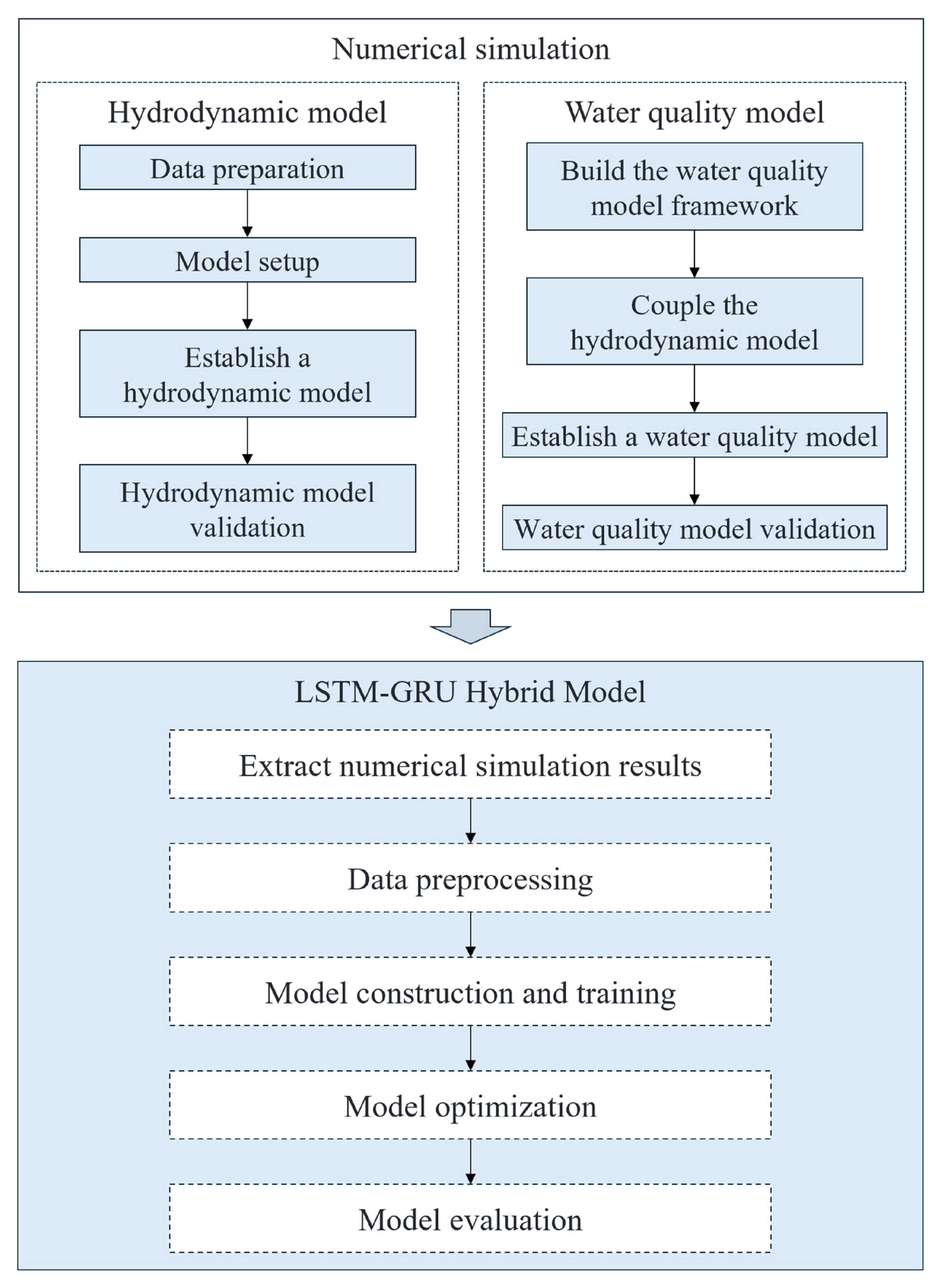
This study constructs an LSTM-GRU Hybrid Model to predict the spatiotemporal distribution of DO concentration in Shenzhen Bay. The overall research framework is shown in Figure 1. Firstly, based on the actual conditions of the study area, data preparation is conducted, including the collection of necessary hydrodynamic data. The model setup is performed by selecting appropriate physical parameters, and a hydrodynamic model is established based on Delft3D FM (Deltares, Delft, The Netherlands). The model is then validated to ensure the accuracy and reliability of the hydrodynamic simulation results. Building upon the existing hydrodynamic model, a water quality model framework is further developed, with dissolved oxygen as the primary water quality factor for simulation, followed by model validation. Based on the numerical simulation results from the hydrodynamic and water quality models, the LSTM-GRU Hybrid Model is constructed. The dissolved oxygen concentration data from four key boundary points in the research area over the past six days are used as input (the statistical characteristics of the input and target variables are shown in

Table 1. Statistics of Input Variables and Target Variable.

Statistical Measure	Boundary Point 1 (g O2/m3)	Boundary Point 2 (g O2/m3)	Boundary Point 3 (g O2/m3)	Boundary Point 4 (g O2/m3)	Target Variable (g O2/m3)
Mean	6.65	6.64	6.63	6.58	6.70
Maximum	7.11	7.09	7.30	7.60	7.72
Minimum	5.86	5.85	5.84	5.78	4.92
Standard Deviation	0.29	0.28	0.27	0.28	0.49

). A total of 793,520 data samples are employed to train the machine learning model, which is randomly split by time index into training, validation, and test sets at a ratio of 6:2:2. The model is then applied to predict the spatial distribution of DO concentration across the entire study area. Through model optimization, including adjusting hyperparameters, the final model’s performance is evaluated to ensure that the constructed model has good prediction accuracy and stability.

2.2. Study Area and Data Sources

2.2.1. Study Area

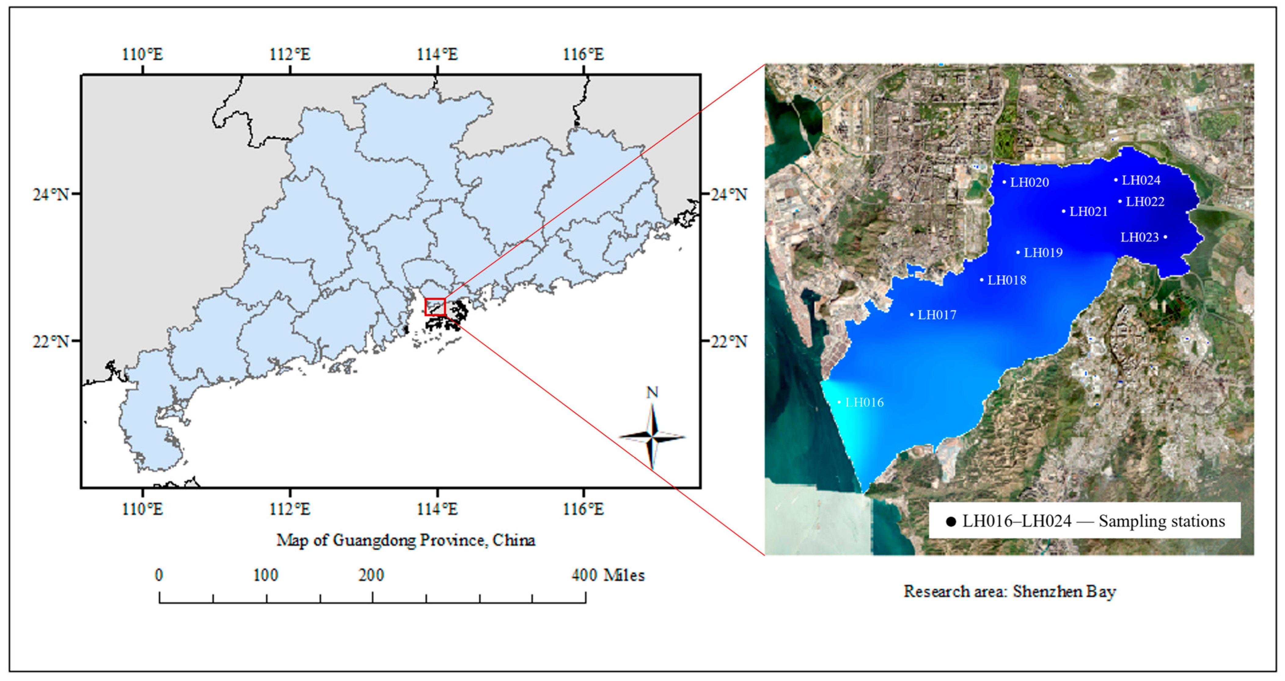
Shenzhen Bay is located in the southern part of Guangdong Province, China, situated between the city of Shenzhen and the Hong Kong Special Administrative Region. It is a typical semi-enclosed water body and is part of the Pearl River Estuary water system. As shown in Figure 2, Shenzhen Bay stretches east to west with a narrow north–south width. It is influenced by the runoff from the Pearl River Estuary, tidal dynamics, land-based runoff inputs, and monsoon climate. The hydrodynamic conditions of Shenzhen Bay are complex, with relatively limited water exchange capacity, making the water quality environment sensitive to changes. In recent years, with the acceleration of urbanization in the region, the population density around Shenzhen Bay has increased, and industrial activities have become more frequent. This has led to an increase in land-based pollutant inputs, resulting in noticeable changes in the spatiotemporal distribution of dissolved oxygen concentration. The water quality situation urgently requires monitoring and improvement. Shenzhen Bay not only has important ecological functions but also serves as a key area for socio-economic activities between Guangdong and Hong Kong. Therefore, in-depth research on the variation patterns of dissolved oxygen concentration in Shenzhen Bay is crucial for improving the management of the bay’s water environment and safeguarding the health of its ecosystem.

2.2.2. Data Sources

The meteorological data and water quality data used in this study were obtained from monitoring stations from October 2021 to June 2022. The daily temperature data and daily relative humidity data were sourced from the Shenzhen Meteorological Bureau’s automatic station monitoring system, while the daily wind speed and direction data, daily cloud cover data, and daily average atmospheric pressure data were provided by the Hong Kong Observatory. Solar radiation data were collected from the Hong Kong Kong-King’s Bay Meteorological Station. Water quality monitoring data were obtained from the Shenzhen Coastal Waters Special Monitoring Table, with monthly monitoring data from nine water quality monitoring points (LH016 to LH024) between October 2021 and June 2022. The locations of these monitoring points are shown in Figure 2. The underwater topography data were sourced from previous studies [35]. The five main river mouths selected for this study are Shenzhen River, Dasha River, Fengtang River, Houhai River, and Xiaosha River. River flow was based on multi-year average runoff data; for rivers without multi-year average runoff data, runoff was estimated based on river width, as shown in

Table 2. Basic Information of River Mouths Discharging into the Sea.

River Name	Average Flow (m3·s−1)	Mouth Width (m)	Longitude	Latitude
Shenzhen River	9.91	200	114.035	22.5065
Fengtang River	1.78	36	114.014	22.5292
Dasha River	2.88	80	113.951	22.5222
Xiaosha River	0.58	11.8	113.989	22.5257
Houhai River	1.17	23.62	113.939	22.4892

.

2.3. Physical Representation

The governing equations of the Delft3D hydrodynamic and water quality models in the vertical sigma coordinate system and horizontal curvilinear coordinate system are as follows:

(1)

Continuity equation

$${\displaystyle \frac{\partial \zeta }{\partial t}}+{\displaystyle \frac{1}{\sqrt{G_{\xi \xi }}\sqrt{G_{\eta \eta }}}}{\displaystyle \frac{\partial ((d+\zeta )u\sqrt{G_{\eta \eta }})}{\partial \xi }}+{\displaystyle \frac{1}{\sqrt{G_{\xi \xi }}\sqrt{G_{\eta \eta }}}}{\displaystyle \frac{\partial ((d+\zeta )v\sqrt{G_{\xi \xi }})}{\partial \eta }}=(d+\zeta )Q$$

(1)

In the equation, u and v represent the flow velocities in the ξ and η directions, respectively (unit: m·s⁻¹); Q denotes the flow rate change per unit area due to drainage or precipitation (unit: m·s⁻¹); d is the depth below the reference surface (unit: m), ζ represents the free surface elevation above the reference plane (unit: m), and d + ζ is the total water depth (unit: m); t denotes time (unit: s).

(2)

Momentum equation

The momentum equation in the ξ direction is:

$$\begin{array}{l}{\displaystyle \frac{\partial u}{\partial t}}+{\displaystyle \frac{u}{\sqrt{G_{\xi \xi }}}}{\displaystyle \frac{\partial u}{\partial \xi }}+{\displaystyle \frac{v}{\sqrt{G_{\eta \eta }}}}{\displaystyle \frac{\partial u}{\partial \eta }}+{\displaystyle \frac{\omega }{d+\zeta }}{\displaystyle \frac{\partial u}{\partial \sigma }}-{\displaystyle \frac{v^2}{\sqrt{G_{\xi \xi }}\sqrt{G_{\eta \eta }}}}{\displaystyle \frac{\partial \sqrt{G_{\eta \eta }}}{\partial \xi }}+{\displaystyle \frac{uv}{\sqrt{G_{\xi \xi }}\sqrt{G_{\eta \eta }}}}{\displaystyle \frac{\partial \sqrt{G_{\xi \xi }}}{\partial \eta }}\\ -fv=-{\displaystyle \frac{1}{{\rho }_0\sqrt{G_{\xi \xi }}}}{P}_{\xi }+F_{\xi }+{\displaystyle \frac{1}{{(d+\zeta )}^2}}{\displaystyle \frac{\partial }{\partial \sigma }}({\upsilon }_v{\displaystyle \frac{\partial u}{\partial \sigma }})+M_{\xi }\end{array}$$

(2)

The momentum equation in the η direction is:

$$\begin{array}{l}{\displaystyle \frac{\partial v}{\partial t}}+{\displaystyle \frac{u}{\sqrt{G_{\xi \xi }}}}{\displaystyle \frac{\partial v}{\partial \xi }}+{\displaystyle \frac{v}{\sqrt{G_{\eta \eta }}}}{\displaystyle \frac{\partial v}{\partial \eta }}+{\displaystyle \frac{\omega }{d+\zeta }}{\displaystyle \frac{\partial v}{\partial \sigma }}-{\displaystyle \frac{u^2}{\sqrt{G_{\xi \xi }}\sqrt{G_{\eta \eta }}}}{\displaystyle \frac{\partial \sqrt{G_{\xi \xi }}}{\partial \eta }}+{\displaystyle \frac{uv}{\sqrt{G_{\xi \xi }}\sqrt{G_{\eta \eta }}}}{\displaystyle \frac{\partial \sqrt{G_{\eta \eta }}}{\partial \xi }}\\ -fu=-{\displaystyle \frac{1}{{\rho }_0\sqrt{G_{\eta \eta }}}}{P}_{\eta }+F_{\eta }+{\displaystyle \frac{1}{{(d+\zeta )}^2}}{\displaystyle \frac{\partial }{\partial \sigma }}({\upsilon }_v{\displaystyle \frac{\partial v}{\partial \sigma }})+M_{\eta }\end{array}$$

(3)

In the equation, w represents the flow velocity in the vertical direction (unit: m·s⁻¹); σ is the proportional vertical coordinate; ρ₀ is the density of water (unit: kg·m⁻³); P_ξ and P_η represent the hydrostatic pressure gradients in the ξ and η directions, respectively (unit: kg·m⁻²·s⁻²)); F_ξ and F_η represent the effects of horizontal Reynolds stresses causing imbalance in the ξ and η directions, respectively (unit: m·s⁻²); M_ξ and M_η represent the effects of external factors on momentum in the ξ and η directions, respectively (unit: m·s⁻²); ${\upsilon }_v$ is the vertical eddy viscosity coefficient (unit: m·s⁻²).

(3)

Convection-diffusion-reaction equation

$${\displaystyle \frac{\mathit{\partial }C}{\partial t}}+v_x{\displaystyle \frac{\partial C}{\partial x}}-D_x{\displaystyle \frac{{\partial }^{2}C}{\partial x^2}}+v_y{\displaystyle \frac{\partial C}{\partial y}}-D_y{\displaystyle \frac{{\partial }^{2}C}{\partial y^2}}+v_z{\displaystyle \frac{\partial C}{\partial z}}-D_z{\displaystyle \frac{{\partial }^{2}C}{\partial z^2}}=S+f_R(C,t)$$

(4)

In the equation, C is the concentration (unit: gO₂·m⁻³), D_x, D_y, and D_z are the diffusion coefficients in the x, y, and z directions, respectively (unit: m²·s⁻¹); S is the source (unit: gO₂·m⁻³·s⁻¹), and f_R is the reaction term (unit: gO₂·m⁻³·s⁻¹).

2.4. Numerical Experiments

This study uses a structured grid with an average grid size of approximately 150 m. After orthogonality testing, the cosine values of the node angles are all less than 0.02, meeting the model’s accuracy requirements. The vertical dimension uses a sigma coordinate system divided into 10 layers, and the time step is set to 30 s to balance model stability and computational efficiency. The temperature-salinity module selects the Composite model, which comprehensively considers the horizontal temperature distribution, vertical water-atmosphere interface transfer, and solar radiation absorption rate. The initial conditions are set as a cold start, with a water level of 0 m, salinity of 31 ppt, and temperature of 27 °C. The model boundaries include the entrance of Shenzhen Bay and five main river mouths. The boundary water level at the bay entrance is derived from tidal harmonic analysis based on historical data, while salinity and water temperature are taken from the data of the nearshore monitoring point LH016. For the river mouth boundary conditions, the flow is calculated based on the runoff data (see Table 1), and water quality data are organized based on river water quality evaluation data. Regarding model parameters, the horizontal eddy viscosity and diffusion coefficient are both 1 m²·s⁻¹, and the vertical eddy viscosity and diffusion coefficient are both 5 × 10⁻⁵ m²·s⁻¹. 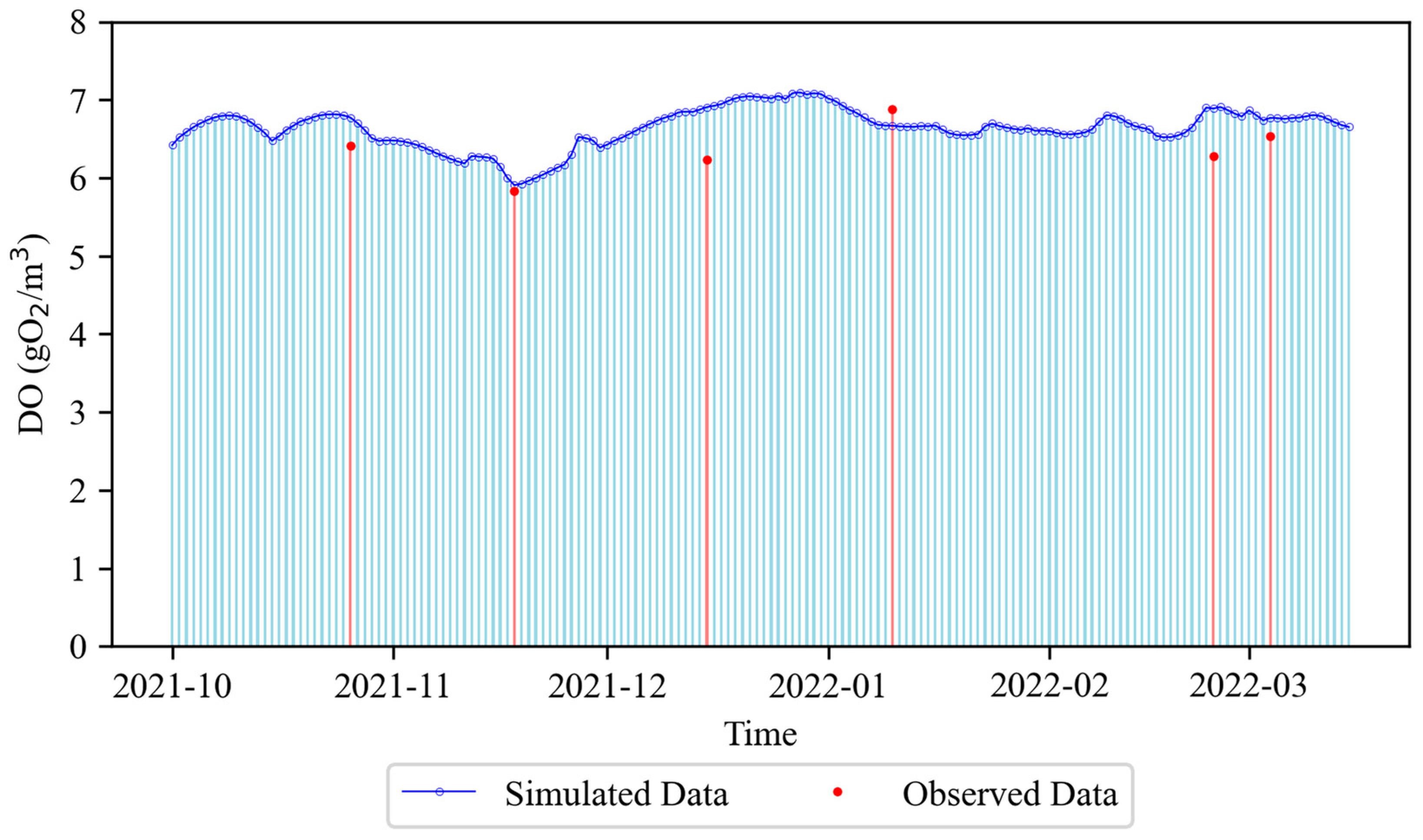The gravitational acceleration is set to 9.81 m·s⁻², and the water density is 1000 kg·m⁻³. The water transparency is represented by a Secchi depth of 2 m, and the meteorological conditions are based on daily meteorological data from October 2021 to June 2022. The water quality model selects dissolved oxygen as the simulated substance, coupled with hydrodynamic simulation results. The initial conditions are obtained through spatial interpolation of the monitoring data from LH016 to LH024, and the dissolved oxygen boundary conditions at the bay entrance and river mouths are set according to water quality observation data.

2.5. LSTM-GRU Hybrid Model

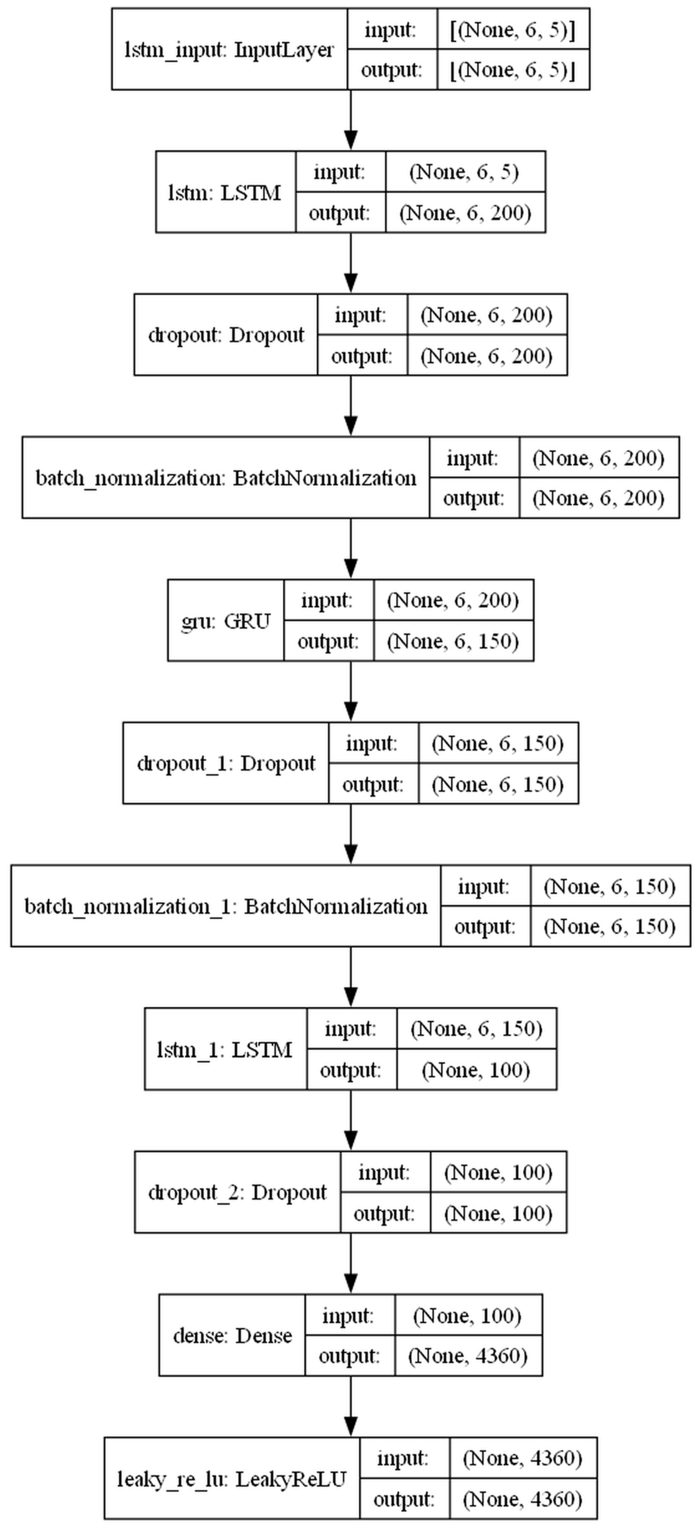
This study develops the LSTM-GRU Hybrid Model to predict the distribution of dissolved oxygen concentration in the Shenzhen Bay area. The LSTM-GRU Hybrid Model combines the advantages of LSTM networks and GRU networks to enhance the spatiotemporal sequence modeling capability and prediction accuracy. The model architecture is shown in Figure 3, and the hyperparameter settings are provided in

Table 3. Hyperparameter settings of the LSTM-GRU Hybrid Model.

Hyperparameter	Settings
N_timesteps	6
LSTM layer neuron count	200, 100
GRU layer neuron count	150
Dropout	0.5
Activation function	tanh + LeakyReLU(0.05)
Optimizer	RMSprop
Learning rate	0.001
Epochs	800

Note: The hardware environment for the computations in this study is: 13th Gen Intel(R) Core(TM) i5-13400F 2.50 GHz, 16 GB RAM, and a 64-bit operating system.

. The model architecture achieves temporal feature extraction through a three-layer cascading structure of LSTM(200)-GRU(150)-LSTM(100). The first layer, LSTM, utilizes 200 neurons and retains the full time-step output to capture long-term dependencies. As the core feature extraction layer, the 200 neurons provide sufficient parameter capacity, preventing underfitting caused by an insufficient number of units and ensuring the capture of subtle temporal variations. The intermediate GRU layer with 150 units preserves the computational efficiency of GRU while forming a parameter-decreasing structure with the preceding LSTM, thereby reducing feature redundancy. The final layer, LSTM, compresses the time dimension with 100 neurons and outputs the final time-step features. Serving as the feature integration layer, it fuses and refines the features extracted from the previous two layers, with 100 neurons enabling a focus on the most critical temporal representations. To prevent overfitting, a Dropout (0.5) and Batch Normalization layer are inserted after each recurrent network layer, enhancing the model’s generalization through random neuron deactivation and feature distribution standardization. The training process uses the RMSprop optimizer combined with an Early Stopping strategy, dynamically optimizing the mean squared error loss within 800 epochs. This model efficiently models complex time series patterns by leveraging the advantages of hybrid networks, regularization constraints, and adaptive training mechanisms.

2.6. Reference Methods

To ensure the fairness of the ablation experiments, all deep learning baseline models were trained with consistent hyperparameter settings: the LeakyReLU activation function was adopted, mean squared error (MSE) was used as the loss function, the Adam optimizer was employed for parameter updates, the maximum number of training epochs was set to 800, and model performance was monitored on the validation set to prevent overfitting. The only differences among the models lie in their network architectures, which are described in detail below.

2.6.1. LSTM Model

This paper uses the standard Long Short-Term Memory (LSTM) model as a reference algorithm to predict the distribution of dissolved oxygen concentrations in the Shenzhen Bay area. The network architecture adopts a two-layer LSTM stacked structure. The first layer of LSTM is configured with 200 neurons and a tanh activation function, retaining the time-step sequence output to facilitate inter-layer information transfer, followed by a Dropout regularization technique to prevent overfitting. The second layer of LSTM is reduced to 150 neurons, outputting the feature vector of the final time step, achieving feature space compression through a decrease in the number of neurons at each layer. The output layer uses a Dense fully connected layer to match the dimensions of the target variable.

2.6.2. MLP Model

The Multi-Layer Perceptron (MLP) model is a typical feedforward neural network composed of multiple layers of neurons, and is a commonly used deep learning model. In this study, the MLP model is introduced as a reference algorithm. The network architecture adopts a two-layer fully connected structure, with the first layer configured with 200 neurons and using the ReLU activation function to achieve nonlinear high-order feature mapping. The second layer reduces the number of neurons to 150, progressively compressing the feature dimensions. Dropout regularization with an 80% high dropout rate is applied after each layer to force neurons to learn independently and suppress overfitting risks. The output layer consists of a Dense fully connected layer matching the target variable dimensions.

2.6.3. KNN Model

K-Nearest Neighbors (KNN) regression is an instance-based learning method that predicts outcomes by calculating the distance between the input sample and the samples in the training set, selecting the nearest neighbors, and then averaging their output results. In this study, the KNN regression model makes predictions based on local similarity in the feature space. Given a test sample, the model searches for the 5 samples in the training set that are closest in Euclidean distance, and uses the arithmetic mean of the target values of these neighbors as the predicted output. The input feature dimensions are consistent with the standardized training set, and the implicit time series are flattened into static feature vectors from the original sequential structure. The model is initialized using KNeighborsRegressor(n_neighbors = 5), which defaults to using Euclidean distance to construct the feature space similarity measure. During training, the standardized training data is fitted to the KNN regression model, and during prediction, the dissolved oxygen concentration field is generated based on the local linear assumption.

2.6.4. RNN Model

The Recurrent Neural Network (RNN) model can handle the temporal dependencies in sequential data through the hidden state propagation mechanism. In this study, the RNN model consists of two layers of SimpleRNN units. The first layer contains 200 neurons, using tanh as the activation function to preserve the full temporal sequence features, followed by a Dropout layer to prevent overfitting. The second layer of the SimpleRNN unit contains 150 neurons, outputting the final timestep features, followed by a Dropout layer. The output layer is a fully connected structure, with the number of nodes matching the target output dimension.

2.7. Performance Metrices

To evaluate the performance of the predictive models, five commonly used statistical indicators were applied, including the coefficient of determination (R²), mean absolute error (MAE), root mean square error (RMSE), standard deviation (SD), and bias (Bias). Their calculation formulas are as follows:

$${\mathrm{R}}^2=1-{\displaystyle \frac{{\displaystyle {\sum }_{i=1}^n}{(y_i-{\widehat{y}}_i)}^2}{{\displaystyle {\sum }_{i=1}^n}{(y_i-\overline{y})}^2}}$$

(5)

$$\mathrm{M}\mathrm{A}\mathrm{E}={\displaystyle \frac{1}{n}}{\displaystyle \sum _{i=1}^n\left|y_i-{\widehat{y}}_i\right|}$$

(6)

$$\mathrm{R}\mathrm{M}\mathrm{S}\mathrm{E}=\sqrt{{\displaystyle \frac{1}{n}}{\displaystyle \sum _{i=1}^n{(y_i-{\widehat{y}}_i)}^2}}$$

(7)

$$\mathrm{S}\mathrm{D}=\sqrt{{\displaystyle \frac{1}{n}}{{\displaystyle \sum _{i=1}^n\left[\left(y_i-{\widehat{y}}_i\right)-\overline{\left(y-\widehat{y}\right)}\right]}}^2}$$

(8)

$$\mathrm{B}\mathrm{i}\mathrm{a}\mathrm{s}={\displaystyle \frac{1}{n}}{\displaystyle \sum _{i=1}^n({\widehat{y}}_i-y_i)}$$

(9)

where $y_i$, ${\widehat{y}}_i$, and $\overline{y}$ denote the observed, predicted, and mean observed values, respectively, and n is the number of samples.

3. Results

3.1. Numerical Results

In this study, tidal harmonic analysis was employed to estimate the water level at the bay mouth, and the multi-year average runoff was used to approximate river inflow. These treatments can capture the fundamental hydrodynamic characteristics of the region over longer time scales, but they are indeed limited in fully resolving daily or even hourly variations during 2021–2022. In addition, the temporal variation in dissolved oxygen concentrations at the boundaries is subject to uncertainties due to monitoring frequency and spatial representativeness. To minimize these uncertainties, a systematic comparative analysis of the simulation results was conducted through numerical model validation, thereby reducing the overall impact of uncertainties on simulation accuracy.

To validate the accuracy of the numerical model, a comparison was made between the observed DO concentrations at the representative monitoring point LH017 in the central area of the study region and the model simulation results, as shown in Figure 4. Overall, the simulation data and observed data exhibit a consistent trend, effectively reflecting the seasonal fluctuations in DO concentrations, with a slight decrease in autumn and winter, followed by a gradual recovery in spring. At multiple sampling points, the simulated values are close to the observed values, indicating the model’s good local fitting ability. Further calculations show that the model’s root mean square error (RMSE) is 0.422 gO₂/m³, the mean absolute error (MAE) is 0.363 gO₂/m³, and the mean absolute percentage error (MAPE) is 5.72%. These results suggest that the constructed water quality model has high accuracy and reliability, making it effective for simulating and predicting water quality changes in the study area, and providing important support for subsequent training of deep learning models.

Figure 5 shows the spatiotemporal distribution of DO concentration in the study area from 1 to 20 November 2021. Overall, the DO concentration in the entire study area mainly remains between 5.0 and 7.0 gO₂/m³, indicating a relatively high level and suggesting good oxygen conditions in the water during this period. Between 1 and 12 November, the DO concentration was higher at the bay mouth, while the inner bay and estuary areas had relatively lower DO concentrations. The DO concentration decreased from the bay mouth to the inner bay and estuary in the direction of tidal flow, indicating that the exchange with the offshore water had a certain positive effect on improving the water quality at the bay mouth. As time progressed, the DO concentration in the bay mouth area showed a decreasing trend, while the DO concentration in the inner bay and estuary gradually increased, resulting in an improvement in the water quality within the bay. The simulation results effectively reveal the evolution of DO concentration at different spatial locations and time points, further validating the reliability of the numerical model. These results can serve as ground truth for training deep learning models.

3.2. Performance of the LSTM-GRU Hybrid Model

To verify the performance of the LSTM-GRU Hybrid Model constructed in this study for predicting the DO concentration field in Shenzhen Bay, a specific moment was randomly selected from the training set, validation set, and test set. The predicted results were compared with the ground truth, as shown in Figure 6, Figure 7 and Figure 8. From the figure, it can be seen that the spatial distribution trends of the model’s predictions are highly consistent with the ground truth across different datasets. The overall concentration gradient changes and the spatial locations of high and low concentration areas are well reproduced. In both the training and validation sets, the model achieves accurate fitting of the gradient distribution from low to high concentrations, successfully capturing the decreasing pattern of DO concentration from the bay mouth to the inner bay, with minimal numerical differences. During the testing phase, where DO concentration exhibits obvious spatial variation, the model still accurately captures the global concentration gradient, reflecting the real concentration distribution. Overall, the proposed LSTM-GRU hybrid model demonstrates good generalization ability and can successfully decouple the spatiotemporal heterogeneity patterns of the DO concentration field in Shenzhen Bay.

Sixteen random points were selected within the study area to create contour plots comparing the LSTM-GRU Hybrid Model with Ground Truth, as shown in Figure 9. The point cluster densely distributed near the diagonal line further demonstrates that the LSTM-GRU Hybrid Model can accurately capture the gradient change pattern of the DO concentration field. The prediction error distribution for different concentration intervals is uniform, with no systematic overestimation or underestimation. It is noteworthy that the model maintains stable prediction performance at different spatial locations, with the RMSE fluctuating around 0.02 gO₂/m³ and R² deviation < 0.08. This further verifies the stability and reliability of the LSTM-GRU Hybrid Model across different times and spatial locations. It can effectively capture the nonlinear variation characteristics of DO concentration and has strong generalization ability in modeling the spatial heterogeneity and dynamic evolution patterns of the DO concentration field under the complex hydrodynamic conditions in Shenzhen Bay.

3.3. Performance of the Reference Methods

Figure 10 shows the residual scatter plots of the reference algorithms on different datasets. From the figure, it can be observed that the KNN model has a higher concentration of residuals, with residuals mainly distributed within the ±0.2 gO₂/m³ range on the training, validation, and test sets. The MAE values are relatively low, but there is a prediction shift in the low dissolved oxygen concentration region (DO < 6 gO₂/m³) due to sparse samples, indicating that it has a certain advantage in fitting local samples. The LSTM model is relatively stable, with the MAE for all datasets consistently maintained within the 0.08–0.09 range, and the residuals are evenly distributed across the full concentration range, without any systematic bias. The RNN model’s prediction accuracy is slightly lower than that of the LSTM model, showing a trend of over-prediction in the low dissolved oxygen concentration range. In contrast, the MLP model performs poorly, with its MAE significantly higher than that of other models. It shows a systematic underestimation in the DO > 6.5 gO₂/m³ region and exhibits residual skew in all datasets, suggesting that its time-series modeling ability and generalization performance are somewhat lacking. Overall, the LSTM model performs best in temporal feature learning and error control, followed by KNN and RNN, while the MLP model has relatively low applicability in this study.

4. Discussion

This study proposes for the construction of an LSTM-GRU Hybrid Model to predict the distribution of DO concentration in semi-enclosed water body. The model fully integrates the advantages of LSTM in modeling long-term temporal dependencies and the superior computational efficiency and convergence speed of the GRU structure. It not only captures long-term dependencies in time series data but also effectively handles noise and nonlinear features in the data, significantly improving the prediction accuracy and stability. This allows for efficient and accurate prediction of DO concentration distribution in the study area. The model not only improves the spatial and temporal resolution of simulations but also provides new ideas and methods for modeling dynamic water quality changes in complex coastal environments.

Compared to traditional experimental measurements and CFD numerical simulations, machine learning methods offer significant advantages in this study. Traditional in situ monitoring relies on discrete point sampling, which is limited by the density of device deployment and measurement frequency, making it difficult to achieve high-frequency observation over large-scale spatial regions and long time periods. CFD methods can simulate hydrodynamic-ecological coupling processes, but their computational efficiency is constrained by grid resolution, parameterization schemes, and boundary condition uncertainties. In complex water bodies like Shenzhen Bay, which are affected by multiple factors such as tides, runoff, and pollution discharge, CFD simulations can take hours to complete. In contrast, the LSTM-GRU Hybrid Model, through a data-driven approach, learns the spatiotemporal correlations in the data, enabling the analysis of nonlinear interactions without explicitly constructing physical equations. This reduces the prediction time to seconds while maintaining prediction accuracy, improving computational efficiency by one order of magnitude and demonstrating its strong potential to replace and supplement traditional methods.

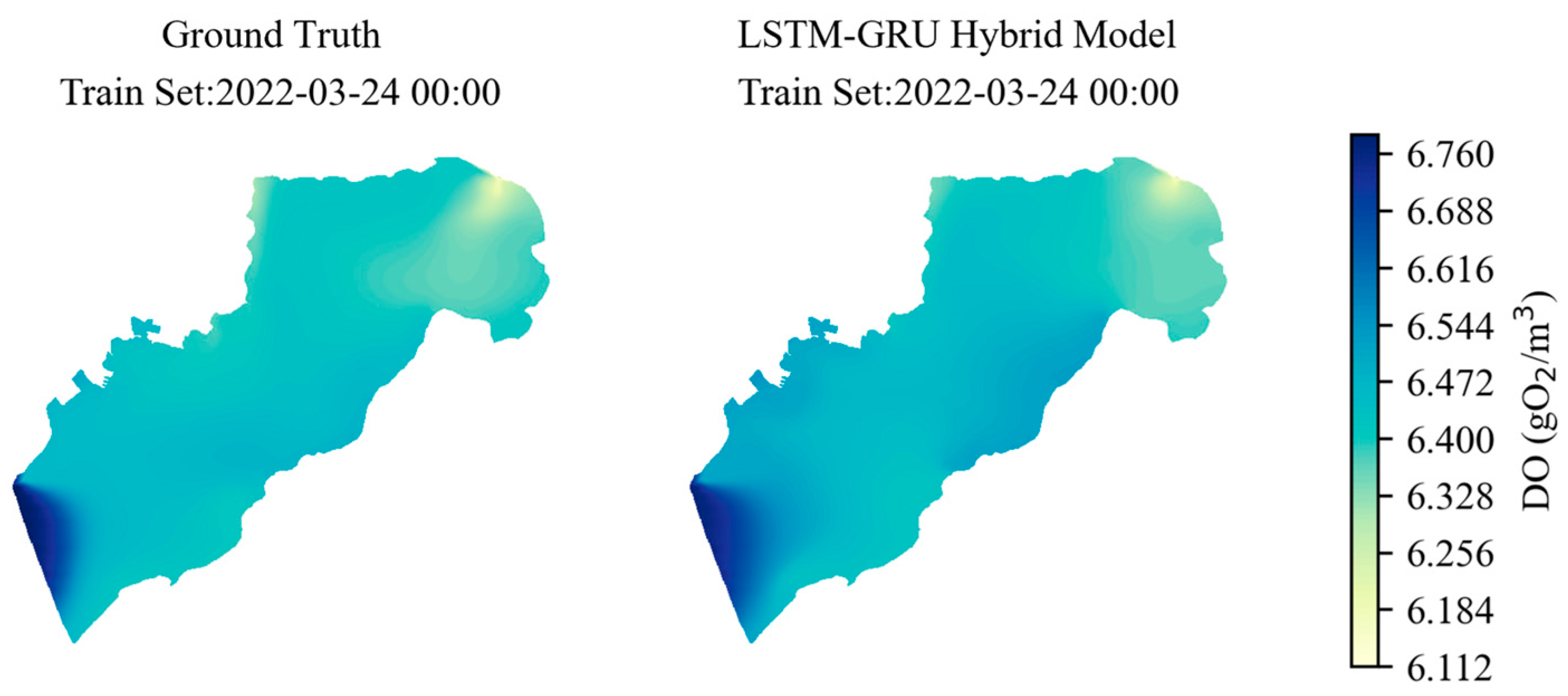
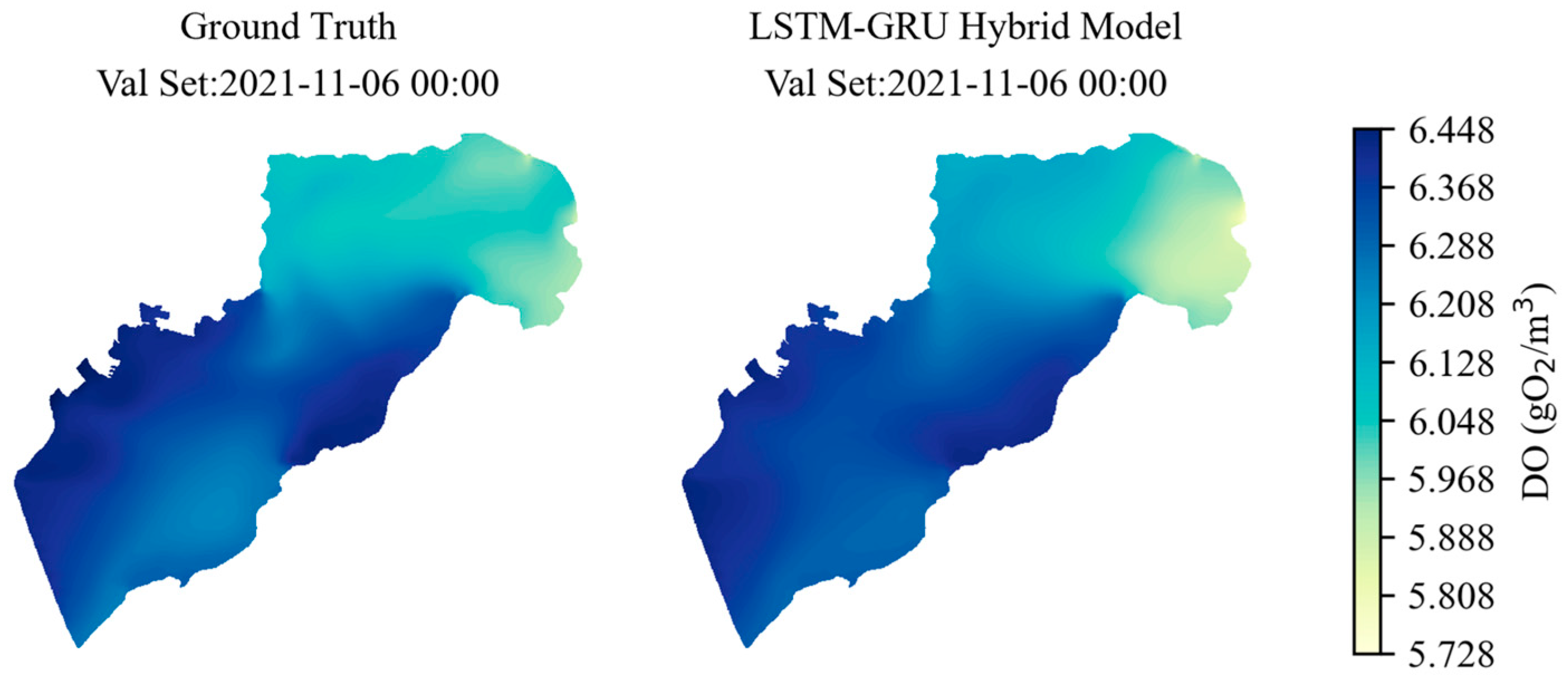
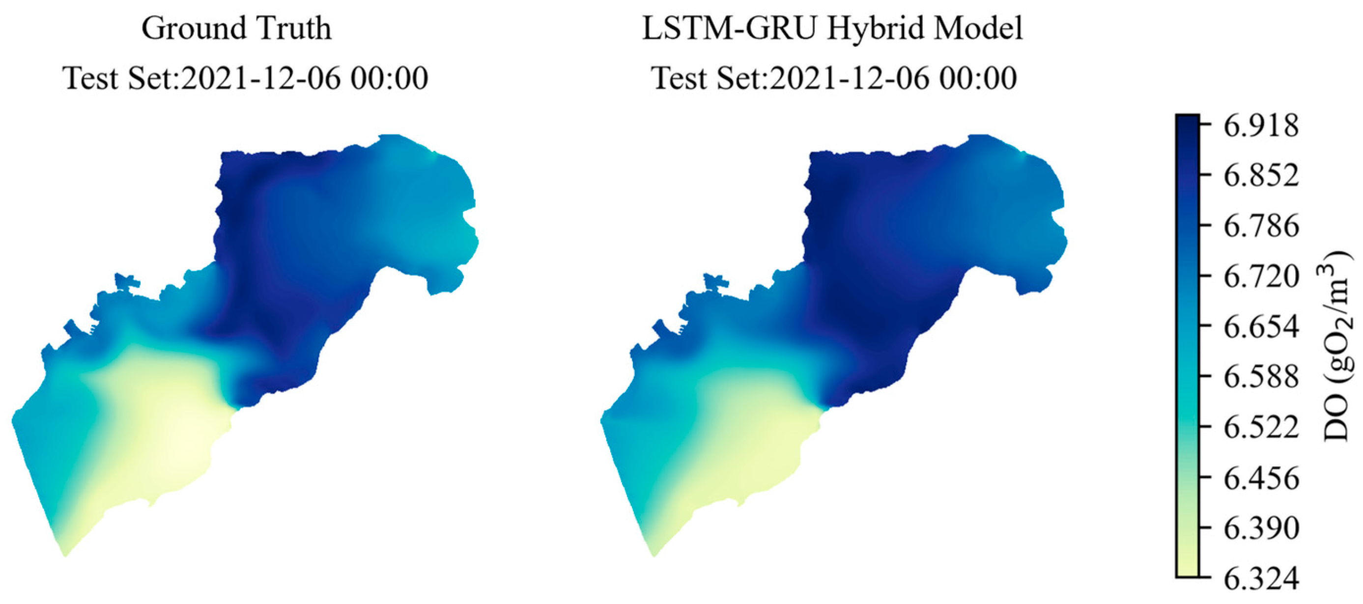
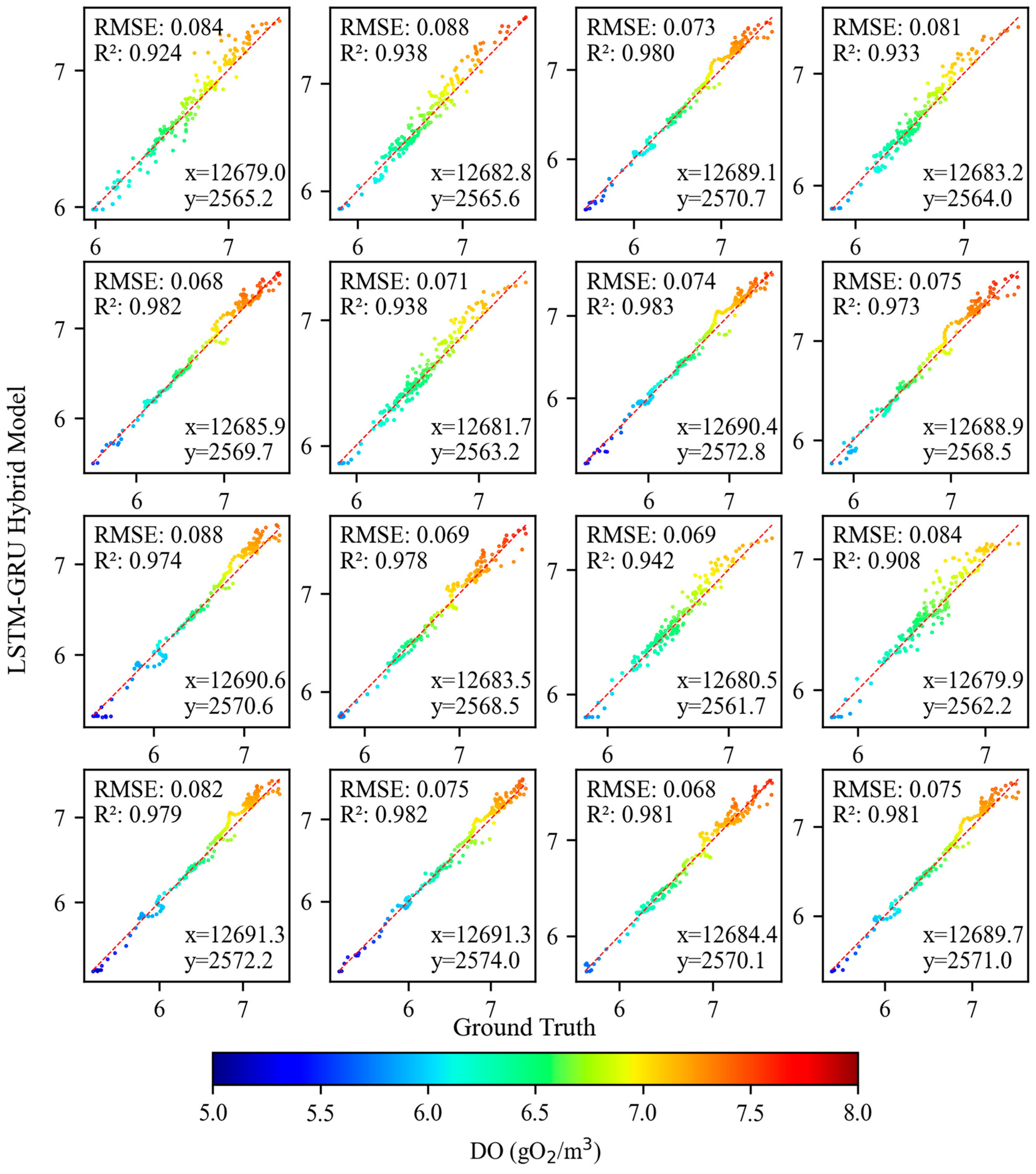
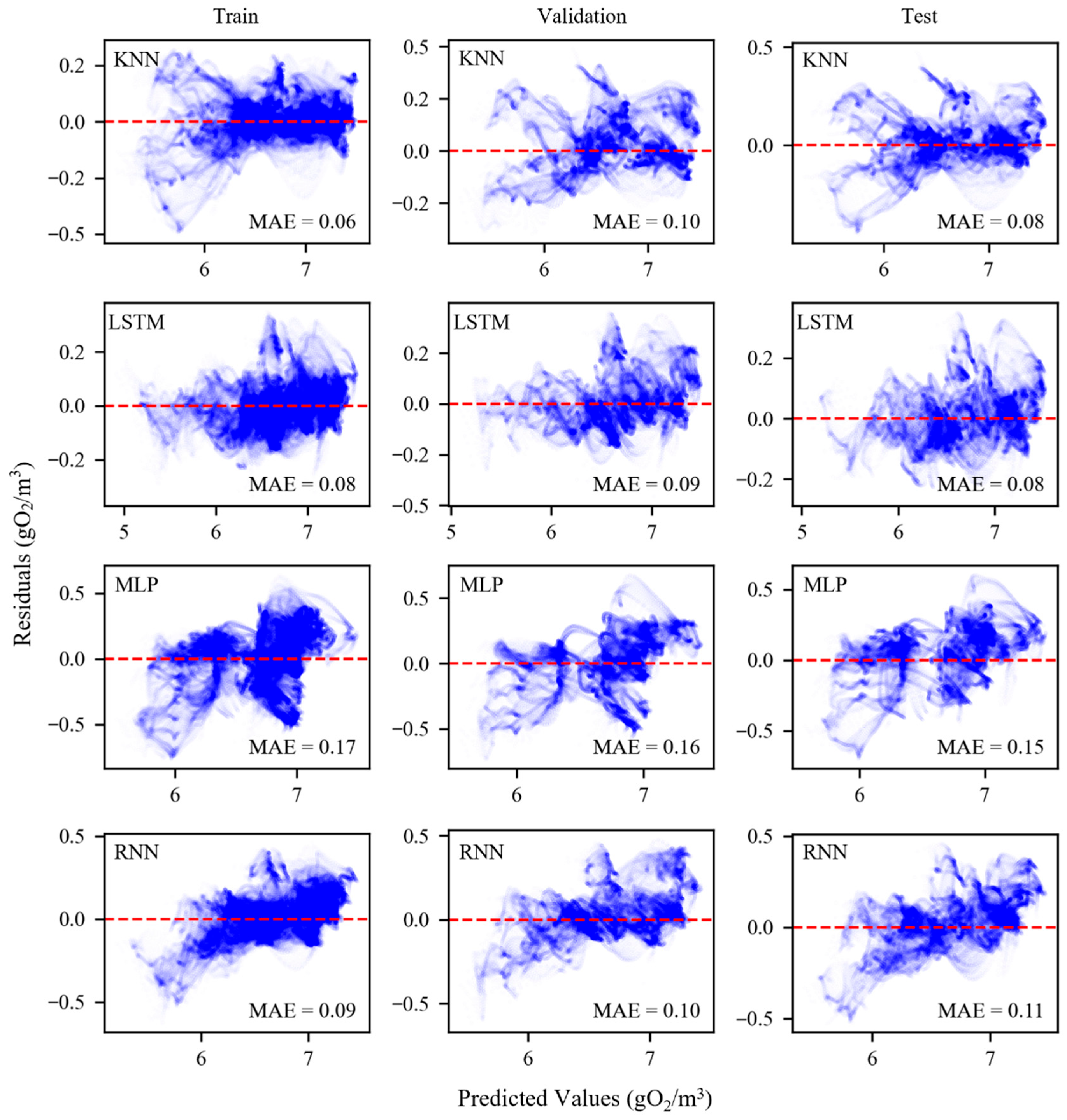
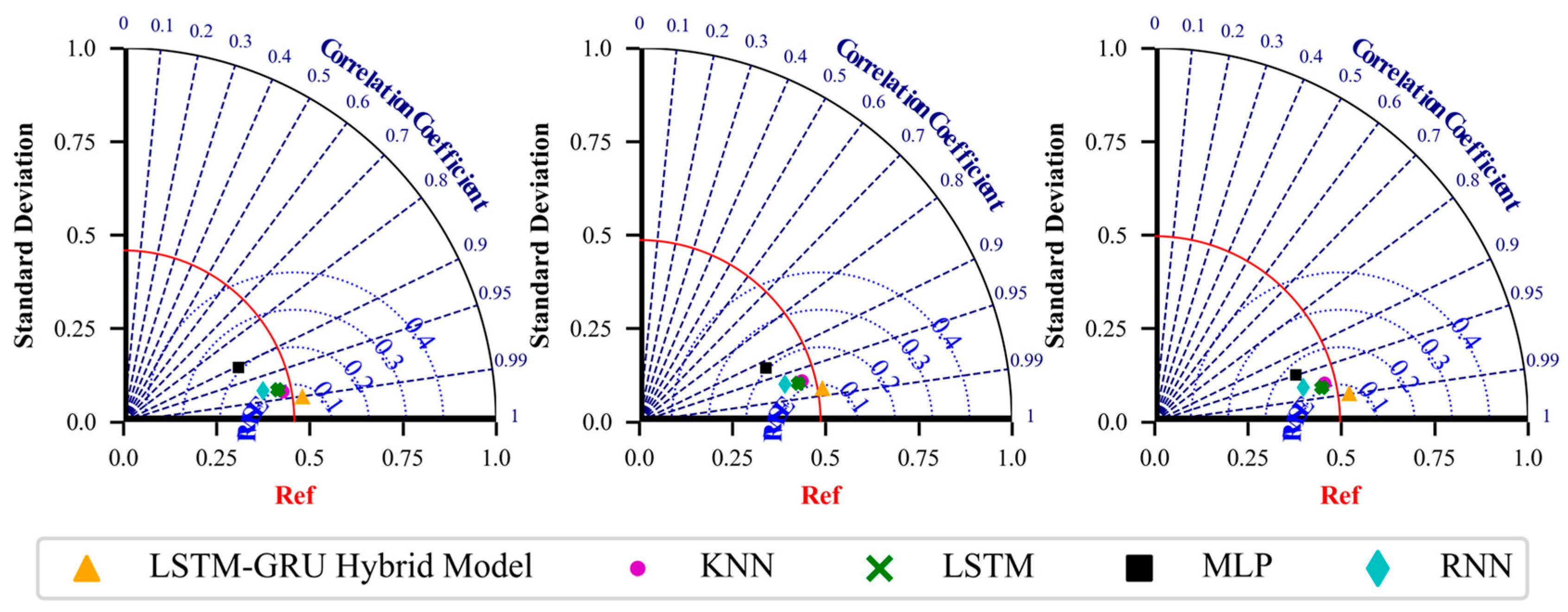
Compared to other machine learning models, such as KNN, MLP, RNN, and LSTM models, the LSTM-GRU Hybrid Model shows significant advantages in the training, validation, and testing stages, as shown in Figure 11, the error metrics of each algorithm are presented in

Table 4. Performance of each model.

Dataset	Metrics	LSTM-GRU	KNN	LSTM	MLP	RNN
Train	R2	0.976	0.964	0.954	0.789	0.931
	RMSE	0.070	0.087	0.098	0.211	0.121
	SD	0.483	0.435	0.423	0.341	0.384
	MAE	0.054	0.062	0.076	0.170	0.092
	Bias	0.025	−0.007	0.001	−0.017	−0.019
Validation	R2	0.968	0.934	0.940	0.818	0.913
	RMSE	0.087	0.125	0.120	0.208	0.144
	SD	0.499	0.450	0.439	0.369	0.403
	MAE	0.069	0.095	0.091	0.164	0.104
	Bias	0.018	−0.032	−0.007	−0.007	−0.032
Test	R2	0.972	0.947	0.955	0.866	0.922
	RMSE	0.083	0.114	0.105	0.182	0.139
	SD	0.526	0.467	0.457	0.398	0.409
	MAE	0.063	0.083	0.082	0.146	0.105
	Bias	0.033	−0.020	−0.008	−0.055	−0.030

Note: The unit of RMSE, MAE, and SD are gO₂/m³.

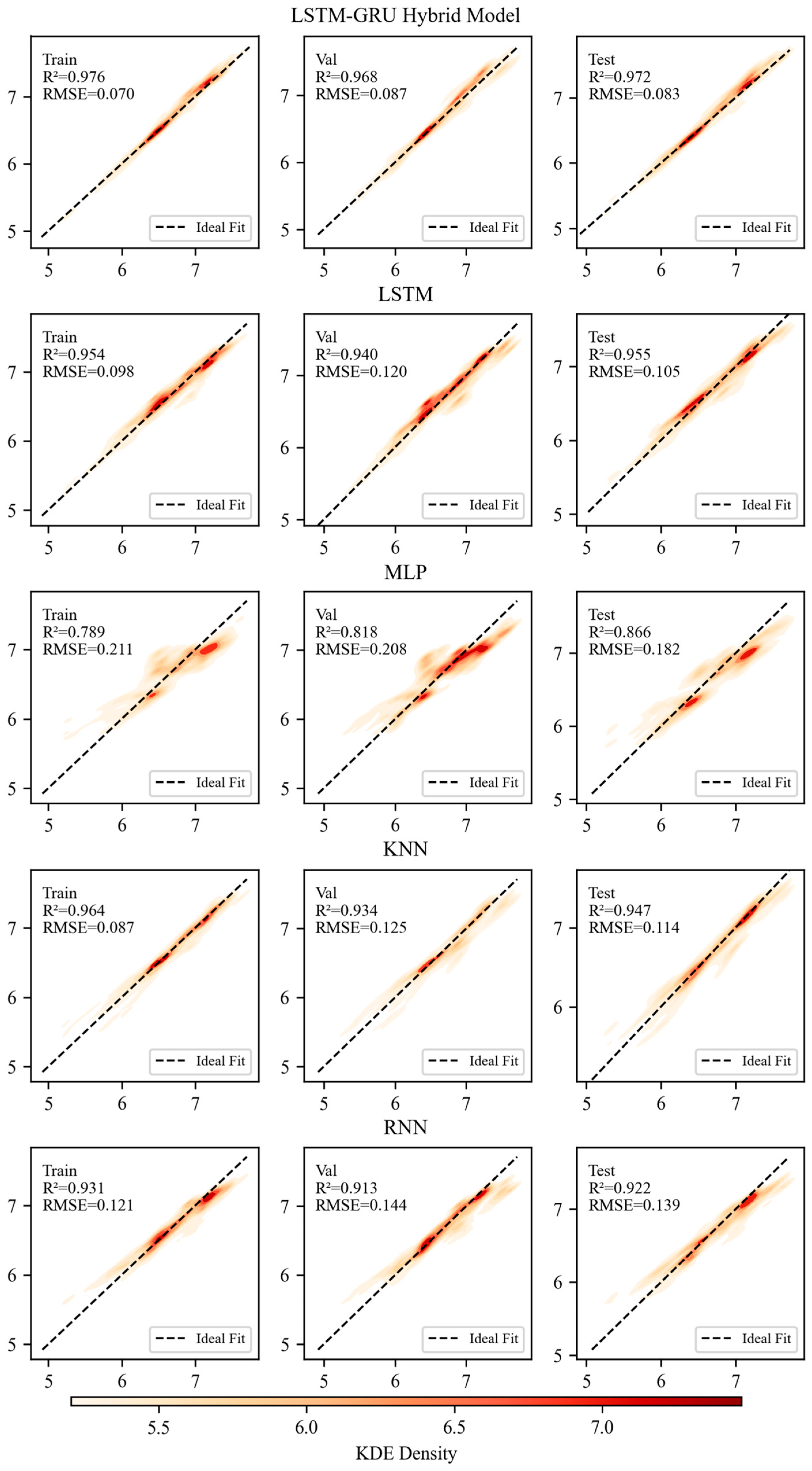
. On all three datasets, the LSTM-GRU Hybrid Model’s standard deviation (SD) is closer to the reference values, its R² is closer to 0.99, and its RMSE is below 0.09 gO₂/m³, indicating superior fitting ability and prediction accuracy for dissolved oxygen concentration. In comparison, the performance of KNN, MLP, RNN, and LSTM models is slightly inferior. Figure 12 shows the kernel density estimation of each algorithm. The LSTM-GRU Hybrid Model significantly outperforms the other models, with its predicted values closely concentrated near the ideal fit line, and the error distribution is relatively small. This further validates the superiority of the LSTM-GRU Hybrid Model in modeling dissolved oxygen concentration in semi-enclosed water body. This advantage may be attributed to the complementary nature of LSTM and GRU structures. LSTM excels in handling long-term dependencies, while GRU performs better in training efficiency and convergence speed. The combination of the two alleviates overfitting and training complexity while maintaining prediction accuracy. In this study, the LSTM-GRU Hybrid Model shows a convergence speed comparable to other reference models, but demonstrates stronger expressive power in feature extraction and temporal modeling, better adapting to the complex hydrodynamics and biogeochemical processes of Shenzhen Bay, thus improving overall prediction performance.

In addition, this study compares its results with existing machine learning research. For example, Kim et al. [36] employed an LSTM model to predict the British Columbia Water Quality Index (BCWQI) in Lake Päijänne, Finland, and the results showed that the model outperformed ANN, SVR, and RF, achieving an R² of 0.91 and an RMSE of 0.11. Similarly, this study verifies the advantages of deep learning in capturing the nonlinear dynamic characteristics of water bodies. Compared with the standalone LSTM model, however, the proposed LSTM-GRU Hybrid Model further improves prediction accuracy and stability, achieving an R² close to 0.99 and an RMSE below 0.09 gO₂/m³ in DO prediction for semi-enclosed coastal areas. This demonstrates its stronger adaptability and robustness in highly nonlinear and noisy marine environments.

This study achieved good prediction results in simulating dissolved oxygen concentration in the Shenzhen Bay area and validated the effectiveness of the LSTM-GRU Hybrid Model. However, the model primarily relies on data trained under normal conditions and lacks specialized modeling and response mechanisms for abnormal events (such as heavy rainfall, red tides, and other extreme situations). In addition, strong physical forcing factors such as tidal height, current velocity, wind speed, air temperature, salinity, radiation, and river inflow were not explicitly incorporated; instead, the DO concentrations at four key boundary points over the past six days were selected as the primary input. The rationale for this choice is as follows: first, boundary DO concentrations largely integrate the combined effects of water exchange, meteorological conditions, and biological processes, thereby indirectly reflecting the influence of multiple physical and chemical drivers; second, Shenzhen Bay is a semi-enclosed water body with relatively stable hydrodynamic conditions, and the DO time series at boundary points is highly representative of the spatiotemporal distribution throughout the bay; and third, to balance model complexity and generalization capability, simplified input features were adopted to validate the feasibility and effectiveness of prediction under limited driving information. In addition, this study conducted a feature importance analysis, and the contribution rates of the boundary points were 31.6%, 38.6%, 16.3%, and 13.5%, respectively, revealing the differences in the model’s sensitivity to DO concentrations at different boundary points. Future research will further incorporate tidal, salinity, and meteorological data to construct a multimodal input framework, enhance the collection and modeling of extreme event data, and allow the model to maintain good adaptability and robustness even under sudden environmental changes, further promoting the application of intelligent prediction models in water environment simulation and management.

5. Conclusions

This study applies deep learning technology to the spatiotemporal prediction of DO concentration fields in Shenzhen Bay by constructing the LSTM-GRU Hybrid Model, achieving efficient dynamic simulation of water quality parameters in complex semi-enclosed water body. Through a systematic comparison with KNN, RNN, MLP, and the standalone LSTM model, the proposed LSTM-GRU Hybrid Model demonstrates higher correlation coefficients and lower RMSE on the training, validation, and test datasets. The R² value is close to 0.99, and the RMSE is below 0.09 gO₂/m³, fully validating its superiority in complex nonlinear water quality prediction tasks. The LSTM-GRU Hybrid Model provides a new technological approach for environmental modeling and assessment in semi-enclosed water bodies. The research results can offer decision-making support for ecological environment assessments, pollution early warning, and resource scheduling in typical water bodies, such as urban bays. Future research should focus on strengthening extreme event data modeling to enhance the model’s adaptability and robustness, further advancing the application of intelligent prediction.