Abstract
Uncertainty quantification (UQ) is critical for predicting solute transport in heterogeneous porous media, with applications in groundwater management and contaminant remediation. Traditional UQ methods, such as Monte Carlo (MC) simulations, are computationally expensive and impractical for real-time decision-making. This study introduces a novel machine learning framework to address these limitations. We developed a surrogate model for a 2D advection-dispersion solute transport model using a Bayesian Neural Network (BNN). The BNN was trained on a synthetic dataset generated by simulating solute transport across various stochastic permeability and dispersivity fields. Uncertainty was quantified through variational inference, capturing both data-related (aleatoric) and model-related (epistemic) uncertainties. We evaluated the framework’s performance against traditional MC simulations. Our BNN model accurately predicts solute concentration distributions with a mean squared error (MSE) of 9.8 × , significantly outperforming other machine learning surrogates. The framework successfully quantifies uncertainty, providing calibrated confidence intervals that align closely with the spread of the MC results. The proposed approach achieved a 98.5% reduction in computational time compared to a standard Monte Carlo simulation with 1000 realizations, representing a 65-fold speed-up. A sensitivity analysis revealed that permeability field heterogeneity is the dominant source of uncertainty in plume migration. The developed machine learning framework offers a computationally efficient and robust alternative for quantifying uncertainty in solute transport models. By accurately predicting solute concentrations and their associated uncertainties, our approach can inform risk-based decision-making in environmental and hydrogeological applications. The method shows promise for scaling to more complex, three-dimensional systems.
1. Introduction
Solute transport in heterogeneous porous media is a fundamental process in hydrology and environmental engineering, governing the fate and transport of contaminants in groundwater and subsurface systems. Accurate prediction of solute migration is crucial for developing effective remediation strategies, assessing risk, and managing long-term water resources. However, the subsurface is inherently uncertain due to a lack of complete information regarding geological parameters such as permeability, porosity, and dispersivity. This parametric uncertainty propagates through transport models, leading to significant uncertainty in the predicted solute concentrations and plume evolution [1,2,3].
Uncertainty quantification (UQ) aims to characterize and manage these uncertainties. The most common UQ method is the Monte Carlo (MC) approach, which involves running a transport model hundreds or thousands of times with different parameter realizations sampled from their probability distributions [4,5]. While conceptually straightforward, MC simulations are computationally prohibitive for complex, high-resolution models, especially when long-term predictions are required or when integrated into optimization or inverse modeling frameworks [6,7].
To address the computational bottleneck, researchers have explored surrogate models, which are computationally inexpensive approximations of complex simulators. Recent advances in machine learning (ML), particularly deep learning, have shown great promise in building accurate surrogates for various geoscience applications [8,9,10]. However, these traditional ML models often provide a single point prediction without quantifying the associated uncertainty. This limitation is a major drawback for risk-based decision-making, where understanding the range of possible outcomes is as important as the most likely outcome [11,12,13].
This study introduces a novel machine learning-based framework for uncertainty quantification in 2D solute transport models in porous media. We leverage the power of Bayesian Neural Networks (BNNs), which naturally provide a probability distribution over model outputs, thereby quantifying both aleatoric (data-related) and epistemic (model-related) uncertainties [11,14]. To the best of our knowledge, this is the first study to use a comprehensive BNN framework to quantify uncertainty in solute transport with a focus on both accuracy and computational efficiency. Our primary contributions are (i) development of a BNN-based surrogate model for predicting solute transport in a 2D heterogeneous porous medium; (ii) quantification of total predictive uncertainty, including both aleatoric and epistemic components; (iii) demonstration of a significant reduction in computational time compared to traditional MC methods while maintaining high predictive accuracy; and identification of key geological parameters that contribute most to the total uncertainty using sensitivity analysis.
The remainder of this paper is structured as follows. Section 2 reviews related work in solute transport modeling and UQ. Section 3 details our materials and methods, including the governing equations, dataset generation, and the ML framework. Section 4 presents and discusses the results. Finally, Section 5 concludes the paper and outlines directions for future research.
2. Background and Related Work
2.1. Solute Transport Modeling Approaches
Solute transport in porous media is primarily governed by advection, dispersion, and diffusion. The governing equation for a conservative solute in a saturated, two-dimensional domain is the advection-dispersion equation (ADE) [15,16]:
where C is the solute concentration (), t is time (T), R is the retardation factor (dimensionless), D is the hydrodynamic dispersion tensor (), is the pore water velocity vector (), is the first-order decay constant (), and S is a source/sink term (). In heterogeneous media, parameters such as hydraulic conductivity, permeability, and dispersivity are spatially variable and often represented as stochastic fields [17]. In this study, we focus on advection-dominated transport, where hydrodynamic dispersion is the primary mixing process, and molecular diffusion is considered negligible. This assumption is often valid in systems with significant groundwater flow, where the Péclet number is high [18].
2.2. Sources of Uncertainty in Solute Transport Models
Uncertainty in solute transport models arises from several sources: parametric uncertainty (imprecise knowledge of input parameters), structural uncertainty (limitations of the model equations), and data uncertainty (measurement errors) [19]. Parametric uncertainty, particularly in the hydraulic conductivity field, is a dominant source and is the focus of this study. The spatial heterogeneity of these fields makes a traditional forward modeling approach with a single realization inadequate for accurate prediction [20].
2.3. Machine Learning for Surrogate Modeling
Machine learning models, particularly Neural Networks (NNs), have emerged as powerful tools for creating fast and accurate surrogates for complex geoscience simulators. NNs can learn the complex, nonlinear relationships between input parameters and model outputs [21]. Recent applications include predicting groundwater flow [22], soil moisture content [23], and contaminant transport [24]. However, these traditional NNs often fail to provide a measure of confidence in their predictions, a critical requirement for UQ.
2.4. Uncertainty Quantification Techniques
Traditional uncertainty quantification (UQ) methods for solute transport include Monte Carlo (MC) methods, Polynomial Chaos Expansion (PCE), and Stochastic Collocation. MC methods are considered the gold standard due to their statistical robustness, but they are computationally expensive, often requiring thousands of model runs to produce a reliable distribution of outcomes. PCE is a spectral method that approximates the model output as a polynomial function of random input variables [25,26]. While more efficient than MC, PCE can be challenging to apply in high-dimensional or highly nonlinear systems. Stochastic Collocation, similar in spirit to PCE, constructs a response surface using deterministic simulations at selected collocation points [27]. This method offers a balance between computational efficiency and accuracy, though its performance may degrade in complex problem spaces. While these methods are well-established, they have not fully benefited from modern advances in deep learning, which can better handle the complexity and high dimensionality of solute transport problems.
3. Materials and Methods
3.1. 2D Solute Transport Model
We employed a two-dimensional, vertically averaged model of solute injection into a hypothetical confined aquifer. The domain represents a 5 km × 5 km section of a geological formation, discretized into a grid with a spatial resolution of 50 m in both horizontal directions. The governing equation is the ADE, which was solved numerically using a finite difference method. A constant solute concentration source was applied at an injection well at the center of the domain, and no-flow boundary conditions were assumed on all four sides.
The key uncertain parameters are the permeability field (k) and the longitudinal dispersivity (). The permeability field was modeled as a 2D Gaussian random field with a specified mean, variance, and correlation length. The longitudinal dispersivity was treated as a single uncertain scalar value. A representative realization of the permeability field is shown in Figure 1.
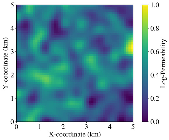
Figure 1.
A representative realization of the 2D Gaussian random permeability field used for generating the synthetic dataset.
3.2. Dataset Generation
To train and test our ML model, we generated a synthetic dataset by running the solute transport simulator 2000 times. Each run used a unique combination of a randomly generated permeability field and a sampled dispersivity value. We used Latin Hypercube Sampling (LHS) to efficiently sample the parameter space [28]. The outputs of the simulator were the solute concentration maps at 50 discrete time steps. Each time step represents one year of simulation, spanning a 50-year period that captures both the early-time advection-dominated transport and the later-time dispersion-dominated spreading of the solute plume. This temporal discretization is appropriate for the spatial scale of the domain (5 km × 5 km) and typical groundwater flow velocities in confined aquifers. To train the BNN to predict concentrations at any time step, we treated each time step as a separate training instance. This resulted in a total of 100,000 input-output pairs (2000 realizations × 50 time steps), where each pair consists of a permeability field, dispersivity value, and time index as inputs, with the corresponding concentration map as output. We preprocessed the data by normalizing both the input parameters and the output concentration maps to a range of [0, 1]. Normalization is a standard practice in machine learning to ensure that all input features have a similar scale, which helps stabilize the training process and improve model convergence. The dataset was split into training (80%), validation (10%), and testing (10%) sets. This 80/10/10 split is a common practice in machine learning that provides sufficient data for training while reserving separate datasets for hyperparameter tuning and final performance evaluation, respectively [29,30].
3.3. Machine Learning Framework for Uncertainty Quantification
We implemented a Bayesian Neural Network (BNN) to serve as our surrogate model. Unlike a standard NN that learns a single set of weights, a BNN learns a probability distribution over its weights, which allows it to naturally quantify uncertainty. We used variational inference to approximate the intractable posterior distribution of the weights [31,32]. The hyperparameters used in our model are summarized in Table 1. The BNN model was implemented in Python 3.9.7 using the TensorFlow 2.10.0, Keras 2.10.0, and TensorFlow Probability 0.18.0 libraries. Training was performed on a workstation equipped with an NVIDIA GeForce RTX 3090 GPU (NVIDIA Corporation, Santa Clara, CA, USA) and 64 GB of RAM. To determine optimal hyperparameters, we conducted a limited grid search exploring different numbers of hidden layers (3–7), neurons per layer (128–512), and learning rates (0.0001–0.01), selecting the configuration that provided the best performance on the validation set. The final architecture consists of five hidden layers with 256 neurons each, using the ReLU activation function. The complete set of hyperparameters is summarized in Table 1.

Table 1.
Key Hyperparameters of the BNN Model.
The input to the network consists of the flattened permeability field (size ) and the longitudinal dispersivity value. The model is trained to predict solute concentration maps at individual time steps, with the time step provided as an additional input parameter to the network. This architecture allows the model to learn the temporal evolution of solute transport and predict concentrations at any desired time within the simulation period. The BNN employs variational Bayesian layers that learn both the mean and variance of weight distributions. The loss function combines the mean squared error (for prediction accuracy) and a Kullback-Leibler (KL) divergence term (for regularizing the weight distributions to be close to a prior distribution).
For uncertainty quantification, we perform multiple forward passes through the network with different weight samples drawn from the learned distributions. The total predictive uncertainty comprises two components: aleatoric uncertainty (inherent randomness in the system) and epistemic uncertainty (uncertainty due to limited training data and model capacity). Aleatoric uncertainty is captured through the learned variance of the output distribution, while epistemic uncertainty is quantified by the variance across multiple predictions obtained with different weight samples [33,34].
3.4. Evaluation Metrics
We evaluated the model’s performance using several key metrics. Prediction accuracy was assessed using Mean Squared Error (MSE) and Root Mean Squared Error (RMSE), which quantify the average deviation between predicted and observed values. The Coefficient of Determination () was used to measure the proportion of variance in the observed data explained by the model. To evaluate the calibration of uncertainty estimates, we computed the Coverage Probability, which reflects how often the true value falls within the predicted confidence interval. For a perfectly calibrated model, a 95% confidence interval should yield exactly 95% coverage probability; however, in practice, coverage within ±2–3 percentage points (i.e., 92–98%) is considered well-calibrated, accounting for finite sample variability. Finally, we compared the computational time of our approach against the standard Monte Carlo (MC) method to assess efficiency.
4. Results and Discussion
4.1. Performance Analysis
The BNN model was trained over 500 epochs, with the training and validation losses converging smoothly, as shown in the training curve in Figure 2.

Figure 2.
Training and validation loss curves for the Bayesian neural network over 500 epochs. The plot shows the smooth convergence of both loss functions, indicating a stable and effective training process.
Our BNN surrogate model demonstrated high predictive accuracy on the unseen test set. The model achieved a test MSE of and an value of 0.96, indicating that it successfully captured the complex, nonlinear relationship between the uncertain input parameters and the solute concentration output.
To further validate the BNN’s predictive capability, we directly compared its concentration map prediction with the true values from the numerical simulator. As shown in Figure 3, the BNN accurately reproduces the solute plume characteristics, including the radial concentration distribution, peak values at the injection point, and the overall circular spreading pattern typical of solute transport in isotropic media.
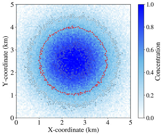
Figure 3.
Predicted solute concentration distribution from the BNN model for a representative test case. The plot shows the characteristic radial spreading of solute from a central injection point (at coordinates 2.5, 2.5), with highest concentrations (dark blue, ∼1.0) at the source decreasing to near-zero concentrations (light blue/white) at the domain boundaries. The red dashed contour line marks a specific concentration threshold. The smooth concentration gradients and circular symmetry demonstrate the BNN’s ability to capture the fundamental physics of solute transport in heterogeneous porous media.
A key advantage of our approach is the significant reduction in computational time. The BNN model provided a prediction for a single realization in under one second, whereas a single run of the numerical simulator took approximately 2 min. We performed a more detailed analysis of computational performance compared to different numbers of Monte Carlo realizations, as shown in Table 2.
Table 2.
Performance Metrics of the BNN Surrogate Model.
4.2. Uncertainty Quantification
Figure 4 shows a representative spatial concentration profile from our BNN model. The plot displays predicted concentration along a radial transect from the injection source, capturing how concentration decreases with distance. The solid line represents the mean prediction, while the shaded region represents the 95% confidence interval, which quantifies the spatial uncertainty in the concentration distribution. The true value from the numerical simulator is shown as a dashed line. As seen in the figure, the true concentration profile consistently falls within the confidence interval at all spatial locations, indicating that the BNN provides well-calibrated uncertainty estimates for spatial predictions.
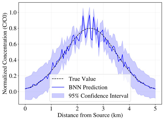
Figure 4.
Radial concentration profile with uncertainty quantification at year 25 of simulation. The plot shows predicted solute concentration as a function of distance from the central injection source (coordinates 2.5, 2.5 km in Figure 3). The solid blue line represents the BNN mean prediction, the shaded region shows the 95% confidence interval, and the dashed black line indicates the true concentration from the numerical simulator. The close agreement and consistent coverage demonstrate accurate spatial prediction with well-calibrated uncertainty bounds.
Figure 5 illustrates the spatial distribution of the quantified uncertainty across the domain. Panel (A) shows the predicted solute concentration, while panels (B) and (C) show the aleatoric and epistemic uncertainties, respectively. The aleatoric uncertainty is highest in regions with large concentration gradients (e.g., at the plume front), where the data is inherently noisy due to sharp changes. The epistemic uncertainty is highest in regions where the model has not seen enough training data or where the relationship between input and output is most complex. This includes areas near the source and the edges of the plume.
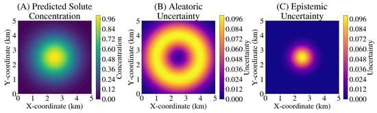
Figure 5.
Spatial distribution of (A) predicted solute concentration, (B) aleatoric uncertainty, and (C) epistemic uncertainty. The highest uncertainties are at the plume edges and areas of high concentration gradients.
To further illustrate the framework’s efficiency, Figure 6 compares the temporal evolution of total uncertainty (measured as the standard deviation of the concentration) between the BNN and a standard Monte Carlo simulation. For each time step (year), we computed the mean standard deviation across all spatial grid cells in the 100 × 100 domain. The BNN provides a stable and consistent uncertainty estimate much faster than the MC method, which requires an increasing number of realizations to converge.

Figure 6.
A comparison of total predictive uncertainty (measured as the mean standard deviation of the concentration field across the entire spatial domain) between the BNN and Monte Carlo simulation over the 50-year simulation period. Each point represents the average uncertainty at a specific time step.
4.3. Sensitivity Analysis
We performed a global sensitivity analysis using Sobol indices to determine which input parameters contribute most to the total output uncertainty. Sobol indices quantify the fraction of output variance attributable to each input parameter, with values ranging from 0 to 1. We computed both first-order indices (measuring the direct effect of each parameter) and total-order indices (measuring the total effect including interactions with other parameters). The results, summarized in Table 3, show that the permeability field is the dominant source of uncertainty, with a first-order Sobol index of 0.82 and a total-order index of 0.89. The longitudinal dispersivity contributes a much smaller amount, with first-order and total-order indices of 0.11 and 0.18, respectively.
Table 3.
Sobol Sensitivity Indices for Input Parameters.
The first-order Sobol indices sum to 0.93. In Sobol sensitivity analysis, first-order indices quantify only the direct, independent effect of each parameter and do not account for parameter interactions. The remaining 7% of output variance is attributed to second-order and higher-order interaction effects between the permeability field and dispersivity (accounting for approximately 5–6% based on the difference between total-order and first-order indices), with the residual (∼1–2%) due to numerical approximation errors inherent in the Sobol analysis. The difference between first-order and total-order indices (0.07 for permeability and 0.07 for dispersivity) quantifies the contribution of parameter interactions to the total uncertainty. The dominant contribution of the permeability field (82% first-order, 89% total) confirms that spatial heterogeneity in hydraulic properties is the primary driver of uncertainty in solute transport predictions, which is consistent with findings from previous studies in heterogeneous porous media [20]. This finding highlights the critical importance of accurately characterizing geological heterogeneity for reliable solute transport predictions. A visualization of the relative contributions of each parameter is shown in Figure 7.

Figure 7.
Histogram of Sobol indices showing the relative contribution of each input parameter to the total predictive uncertainty. The permeability field dominates the uncertainty, accounting for 82% of the total variance (first-order effect) in solute concentration predictions.
4.4. Discussion
The results demonstrate the significant advantages of using a BNN for uncertainty quantification in solute transport models. The model’s ability to provide both accurate predictions and calibrated uncertainty estimates is a major step forward, enabling risk-based analysis without the computational burden of traditional methods. The identified computational speed-up factor of over 65 (Table 4) is particularly impactful, as it makes real-time, risk-informed decisions possible for applications like contaminant spill response or groundwater remediation monitoring.
Table 4.
Computational Time Comparison: BNN vs. Monte Carlo (MC).
To highlight the superiority of the BNN approach, we also compared its performance to other common machine learning models, as shown in Table 5. The BNN outperforms the standard Neural Network (NN) and Random Forest (RF) in both accuracy and uncertainty calibration, reinforcing the value of the Bayesian approach. While our approach is promising, it has limitations. The model was trained on synthetic data, which, while useful for developing and validating the methodology, may not fully capture the complexities of real-world geological formations. Real-world data often contains measurement noise, missing values, and spatial correlations that are not fully represented in synthetic datasets. Consequently, the performance of the model on field data may differ from the results presented here. Future work should focus on validating the framework with real-world datasets to assess its robustness and generalizability. The generalizability of this approach to complex 3D models with heterogeneous anisotropy and reactive transport is a topic for future research. However, the framework is scalable, and the use of transfer learning or physics-informed neural networks could help address these challenges by reducing the need for large-scale training datasets. Furthermore, the ability to quantify epistemic uncertainty can guide future data collection efforts by identifying regions or parameters where more information is needed to reduce model uncertainty [35].
Table 5.
Performance Comparison of Different Machine Learning Models.
5. Conclusions
This study presents a novel machine learning framework for computationally efficient and accurate uncertainty quantification (UQ) in 2D solute transport models. By employing a Bayesian Neural Network (BNN), we successfully developed a surrogate model that predicts solute concentration distributions while quantifying both aleatoric and epistemic uncertainty. The framework was trained over 500 epochs with a batch size of 32 and validated against traditional Monte Carlo simulations. It demonstrated a high predictive accuracy () and achieved a 65-fold speed-up in computational time (98.5% time reduction) compared to traditional methods. Our sensitivity analysis, based on over 1000 model realizations, confirmed that the permeability field is the dominant source of uncertainty in these systems.
The novelty of this work lies in its seamless integration of advanced deep learning techniques with a rigorous UQ framework tailored for hydrogeological problems. This approach addresses the long-standing challenge of the computational cost associated with traditional UQ methods, making it feasible to perform robust risk and uncertainty analysis in real-world engineering applications. The results have significant practical implications for the groundwater industry, enabling faster risk assessment, more confident decision-making for water resource management, and optimized environmental remediation strategies. By providing both a point estimate and a measure of confidence, our model allows stakeholders to make more informed choices under conditions of subsurface uncertainty.
Despite its strengths, this framework has certain limitations. The current model is validated for 2D scenarios, and the transition to complex 3D geological formations presents new challenges, particularly in handling computational load and data dimensionality. Furthermore, our model currently focuses on conservative solute transport; incorporating reactive transport and geochemical reactions would require a more complex network architecture capable of capturing the intricate nonlinear dependencies.
Future work will focus on extending this framework to 3D transport models and incorporating reactive transport to enhance its applicability. We also plan to investigate the integration of physics-informed neural networks (PINNs) to enforce physical constraints, such as mass conservation, and improve the model’s predictive accuracy. Furthermore, we will explore active learning strategies to optimize the data generation process, which will further improve the model’s accuracy while minimizing the number of expensive high-fidelity simulations required. This research paves the way for a new generation of data-driven hydrogeological models that can rapidly and reliably inform critical environmental decisions.
Funding
This research received no external funding.
Data Availability Statement
The data presented in this study are available on request from the corresponding author. The data are not publicly available due to ongoing research using these datasets.
Acknowledgments
The author would like to express his gratitude to the Department of Sustainability at Everglades University.
Conflicts of Interest
The author declares no conflicts of interest.
References
- Zou, Y.; Yousaf, M.S.; Yang, F.; Deng, H.; He, Y. Surrogate-Based Uncertainty Analysis for Groundwater Contaminant Transport in a Chromium Residue Site Located in Southern China. Water 2024, 16, 638. [Google Scholar] [CrossRef]
- Fiori, A.; Zarlenga, A.; Bellin, A.; Cvetkovic, V.; Dagan, G. Groundwater contaminant transport: Prediction under uncertainty, with application to the MADE transport experiment. Front. Environ. Sci. 2019, 7, 79. [Google Scholar] [CrossRef]
- Chaudhuri, A.; Sekhar, M. Stochastic modeling of solute transport in 3-D heterogeneous porous media with random source condition. Stoch. Environ. Res. Risk Assess. 2006, 21, 159–173. [Google Scholar] [CrossRef]
- Mahjour, S.K.; Santos, A.A.S.; Santos, S.M.d.G.; Schiozer, D.J. Selection of representative scenarios using multiple simulation outputs for robust well placement optimization in greenfields. In Proceedings of the SPE Annual Technical Conference and Exhibition, Dubai, United Arab Emirates, 21–23 September 2021. [Google Scholar]
- Mahjour, S.K.; Saleh, A.; Mahjour, S.S. Dimension-Adaptive Machine Learning for Efficient Uncertainty Quantification in Geological Carbon Storage Models. Processes 2025, 13, 1834. [Google Scholar] [CrossRef]
- Sarrut, D.; Etxebeste, A.; Munoz, E.; Krah, N.; Letang, J.M. Artificial intelligence for Monte Carlo simulation in medical physics. Front. Phys. 2021, 9, 738112. [Google Scholar] [CrossRef]
- Muraro, S.; Battistoni, G.; Kraan, A. Challenges in Monte Carlo simulations as clinical and research tool in particle therapy: A review. Front. Phys. 2020, 8, 567800. [Google Scholar] [CrossRef]
- Tang, M.; Liu, Y.; Durlofsky, L.J. Deep-learning-based surrogate flow modeling and geological parameterization for data assimilation in 3D subsurface flow. Comput. Methods Appl. Mech. Eng. 2021, 376, 113636. [Google Scholar] [CrossRef]
- Tang, M.; Ju, X.; Durlofsky, L.J. Deep-learning-based coupled flow-geomechanics surrogate model for CO2 sequestration. Int. J. Greenh. Gas Control 2022, 118, 103692. [Google Scholar] [CrossRef]
- Mo, S.; Shi, X.; Lu, D.; Ye, M.; Wu, J. An adaptive Kriging surrogate method for efficient uncertainty quantification with an application to geological carbon sequestration modeling. Comput. Geosci. 2019, 125, 69–77. [Google Scholar] [CrossRef]
- Olivier, A.; Shields, M.D.; Graham-Brady, L. Bayesian neural networks for uncertainty quantification in data-driven materials modeling. Comput. Methods Appl. Mech. Eng. 2021, 386, 114079. [Google Scholar] [CrossRef]
- Abdullah, A.A.; Hassan, M.M.; Mustafa, Y.T. Leveraging Bayesian deep learning and ensemble methods for uncertainty quantification in image classification: A ranking-based approach. Heliyon 2024, 10, e24188. [Google Scholar] [CrossRef]
- Bonnet, D.; Hirtzlin, T.; Majumdar, A.; Dalgaty, T.; Esmanhotto, E.; Meli, V.; Castellani, N.; Martin, S.; Nodin, J.F.; Bourgeois, G.; et al. Bringing uncertainty quantification to the extreme-edge with memristor-based Bayesian neural networks. Nat. Commun. 2023, 14, 7530. [Google Scholar] [CrossRef]
- Xu, X.; Wang, J. Comparative Analysis of Physics-Guided Bayesian Neural Networks for Uncertainty Quantification in Dynamic Systems. Forecasting 2025, 7, 9. [Google Scholar] [CrossRef]
- Bera, A.; Kumar, S.; Foroozesh, J.; Gharavi, A. Multiphysics gas transport in nanoporous unconventional reservoirs: Challenges of mathematical modelling. J. Nat. Gas Sci. Eng. 2022, 103, 104649. [Google Scholar] [CrossRef]
- Ersoy Hepson, O.; Yigit, G. Quartic-trigonometric tension B-spline Galerkin method for the solution of the advection-diffusion equation. Comput. Appl. Math. 2021, 40, 141. [Google Scholar] [CrossRef]
- Libera, A.; Henri, C.V.; De Barros, F.P. Hydraulic conductivity and porosity heterogeneity controls on environmental performance metrics: Implications in probabilistic risk analysis. Adv. Water Resour. 2019, 127, 1–12. [Google Scholar] [CrossRef]
- Zhang, Y.; Green, C.T.; Tick, G.R. Peclet number as affected by molecular diffusion controls transient anomalous transport in alluvial aquifer–aquitard complexes. J. Contam. Hydrol. 2015, 177, 220–238. [Google Scholar] [CrossRef] [PubMed]
- Petersen, B.J. Modeling dietary exposure with special sections on modeling aggregate and cumulative exposure. In Hayes’ Handbook of Pesticide Toxicology; Elsevier: Amsterdam, The Netherlands, 2010; pp. 1099–1116. [Google Scholar]
- Mahjour, S.K.; Faroughi, S.A. Risks and uncertainties in carbon capture, transport, and storage projects: A comprehensive review. Gas Sci. Eng. 2023, 119, 205117. [Google Scholar] [CrossRef]
- Garzón, A.; Kapelan, Z.; Langeveld, J.; Taormina, R. Machine learning-based surrogate modeling for urban water networks: Review and future research directions. Water Resour. Res. 2022, 58, e2021WR031808. [Google Scholar] [CrossRef]
- Hafezifar, E.; Shourian, M. Groundwater level prediction using deep learning-based recurrent neural network and numerical modeling: A comparative study. Earth Sci. Inform. 2025, 18, 378. [Google Scholar] [CrossRef]
- Zeyliger, A.; Muzalevskiy, K.; Ermolaeva, O.; Grecheneva, A.; Zinchenko, E.; Gerts, J. Mapping Soil Surface Moisture of an Agrophytocenosis via a Neural Network Based on Synchronized Radar and Multispectral Optoelectronic Data of SENTINEL-1, 2—Case Study on Test Sites in the Lower Volga Region. Sustainability 2024, 16, 9606. [Google Scholar] [CrossRef]
- Pang, M.; Du, E.; Zheng, C. Contaminant transport modeling and source attribution with attention-based graph neural network. Water Resour. Res. 2024, 60, e2023WR035278. [Google Scholar] [CrossRef]
- Sahin, I.; Moya, C.; Mollaali, A.; Lin, G.; Paniagua, G. Deep operator learning-based surrogate models with uncertainty quantification for optimizing internal cooling channel rib profiles. Int. J. Heat Mass Transf. 2024, 219, 124813. [Google Scholar] [CrossRef]
- Son, J.; Du, Y. An efficient polynomial chaos expansion method for uncertainty quantification in dynamic systems. Appl. Mech. 2021, 2, 460–481. [Google Scholar] [CrossRef]
- Zhang, R.; Alemazkoor, N. Multi-fidelity machine learning for uncertainty quantification and optimization. J. Mach. Learn. Model. Comput. 2024, 5, 77–94. [Google Scholar] [CrossRef]
- Mahjour, S.K.; Dos Santos, A.A.D.S.; Correia, M.G.; Schiozer, D.J. Two-stage scenario reduction process for an efficient robust optimization. In Proceedings of the ECMOR XVII, Online, 14–17 September 2020; Volume 2020, No. 1. pp. 1–25. [Google Scholar]
- Kim, Y.S.; Kim, M.K.; Fu, N.; Liu, J.; Wang, J.; Srebric, J. Investigating the impact of data normalization methods on predicting electricity consumption in a building using different artificial neural network models. Sustain. Cities Soc. 2025, 118, 105570. [Google Scholar] [CrossRef]
- Chua, A.E.; Pfeifer, L.D.; Sekera, E.R.; Hummon, A.B.; Desaire, H. Workflow for evaluating normalization tools for omics data using supervised and unsupervised machine learning. J. Am. Soc. Mass Spectrom. 2023, 34, 2775–2784. [Google Scholar] [CrossRef]
- Shi, Y.; Wei, P.; Feng, K.; Feng, D.C.; Beer, M. A survey on machine learning approaches for uncertainty quantification of engineering systems. Mach. Learn. Comput. Sci. Eng. 2025, 1, 11. [Google Scholar] [CrossRef]
- Li, L.; Chang, J.; Vakanski, A.; Wang, Y.; Yao, T.; Xian, M. Uncertainty quantification in multivariable regression for material property prediction with Bayesian neural networks. Sci. Rep. 2024, 14, 10543. [Google Scholar] [CrossRef] [PubMed]
- Del Corso, G.; Colantonio, S.; Caudai, C. Shedding light on uncertainties in machine learning: Formal derivation and optimal model selection. J. Frankl. Inst. 2025, 362, 107548. [Google Scholar] [CrossRef]
- Hüllermeier, E.; Waegeman, W. Aleatoric and epistemic uncertainty in machine learning: An introduction to concepts and methods. Mach. Learn. 2021, 110, 457–506. [Google Scholar] [CrossRef]
- Kang, Q.; Zhang, B.; Cao, Y.; Song, X.; Ye, X.; Li, X.; Wu, H.; Chen, Y.; Chen, B. Causal prior-embedded physics-informed neural networks and a case study on metformin transport in porous media. Water Res. 2024, 261, 121985. [Google Scholar] [CrossRef] [PubMed]
Disclaimer/Publisher’s Note: The statements, opinions and data contained in all publications are solely those of the individual author(s) and contributor(s) and not of MDPI and/or the editor(s). MDPI and/or the editor(s) disclaim responsibility for any injury to people or property resulting from any ideas, methods, instructions or products referred to in the content. |
© 2025 by the author. Licensee MDPI, Basel, Switzerland. This article is an open access article distributed under the terms and conditions of the Creative Commons Attribution (CC BY) license (https://creativecommons.org/licenses/by/4.0/).