Article

A Robust 3D Fixed-Area Quality Inspection Framework for Production Lines

1
College of Information Sciences and Technology, Donghua University, Shanghai 201620, China
2
Engineering Research Center of Digitized Textile and Apparel Technology, Ministry of Education, Donghua University, Shanghai 201620, China
3
Shanghai Marine Diesel Engine Research Institute, Shanghai 201108, China
*
Author to whom correspondence should be addressed.
Processes 2025, 13(10), 3300; https://doi.org/10.3390/pr13103300
Submission received: 5 September 2025 / Revised: 8 October 2025 / Accepted: 11 October 2025 / Published: 15 October 2025
(This article belongs to the Section Automation Control Systems)

Abstract

Introducing deep learning methods into the quality inspection of production lines can reduce labor and improve efficiency, with great potential for the development of manufacturing systems. However, in specific closed production-line environments, robust and high-quality 3D fixed-area quality inspection is a common and challenging problem due to improper assembly, high data resolution, pose perturbation, and other reasons. In this article, we propose a robust 3D fixed-area quality inspection framework for production lines consisting of two steps: recursive segmentation and one-class classification. First, a Focal Segmentation Module (FSM) is proposed to gradually focus on the areas to be inspected by recursively segmenting the downsampled low-resolution point cloud, thereby ensuring efficient high-resolution segmentation. Moreover, Local Reference Frame (LRF)-based rotation-invariant local feature extraction is introduced to improve the robustness of the proposed method to pose variations. Second, a uniquely designed Semi-Nested Point Cloud Autoencoder (SN-PAE) is proposed to improve data imbalance and hard-to-classify samples. Particularly, we first introduce rotation-invariant feature extraction to a point cloud autoencoder to learn descriptive latent variables, then measure the latent variables using a semi-nested Latent Autoencoding Module (LAM). This avoids unreliable chamfer distance measurement and makes SN-PAE a more robust measurement method. In addition, we implement a set of experiments using solder joints as an example. Compared with PointNet++, the memory usage of recursive segmentation is reduced by 92%, and the time cost is reduced by 97.5%. The recall of SN-PAE on unaligned samples exceeds that of competitors by nearly 30% in the classification stage. The results demonstrate the feasibility and effectiveness of the proposed framework.

1. Introduction

In recent decades, automation technologies have gradually penetrated all aspects of production lines, thereby improving production efficiency. Therefore, the demand has increased for automated quality inspection methods to replace time-consuming, laborious and poorly consistent manual inspections. Deep learning-based methods have shown excellent performance on many public tasks [1,2]. Researchers have also achieved remarkable results in exploring deep learning theory in industrial fields [3,4,5], where ensuring robust and reliable high-quality defect detection in a closed production-line environment is critical. Unlike public tasks where the data distribution is clean and balanced, researchers often need to build additional designs based on local conditions to cope with the challenges brought about by the actual production environment.
In recent years, deep learning methods have promoted the rapid development of deep point learning algorithms [2], while relatively little research has been conducted in industrial production and manufacturing environments. In this paper, we focus on common 3D fixed-area shape defect inspection in a production line, and take automotive radar solder joint inspection as an example. As shown in Figure 1, in the automotive ultrasonic radar assembly line, the inspection station checks the products one by one with a model trained offline and eliminates the products judged as defective. Fixed-area defect detection is a common problem in the manufacturing industry. Unlike publicly available datasets such as ModelNet40 [6], which feature balanced and rich samples and categories, production-line samples are highly similar, requiring single inspection of one or more fixed areas. This is a binary classification task. If any of the areas is defective, the product is determined to be defective, and the data of different categories are unbalanced. We refer to these fixed areas to be detected as focal areas. In the quality inspection process of production lines, the sensors of the inspection station always obtain overall data in one shot for efficiency; then, the inspection methods generally segment the data of instances, followed by a classifier. In such tasks, the following possible common challenges have to be faced.
(1)
Non-ignorable calculation costs from high-resolution data and redundant data: Collecting high-resolution data is the prerequisite to ensure high-quality detection, but high-resolution and redundant data inevitably lead to increased computational effort and additional invalid calculations.
(2)
Poor robustness caused by unaligned poses: Improper assembly and random workpiece placement inevitably lead to pose misalignment. Changes in pose lead to changes in input data, which can easily lead to samples that the model has not seen, making the model unable to remain robust.
(3)
Data imbalance: The data collected from the production line contains more than 85 % normal samples, and the distribution of defects in different instances is also uneven, which leads to an extremely unbalanced dataset.
(4)
Hard-to-classify samples: Determining a defective product as normal leads to false detection, which is unacceptable because of the strict quality standard. However, it is difficult for deep learning-based methods to avoid misclassification because of hard samples.
Although fixed-area defect inspection widely exists in production lines, few suitable methods are designed for it alone. Methods of 3D fixed-area shape defect inspection can be divided into two technical lines: step-by-step approaches and end-to-end approaches. In a single inspection, the sensors first obtain high-resolution overall data from multiple views, where the former usually segment or crop the fixed regions, then make judgments with a classifier. Methods based on Iterative Closest Point (ICP) registration [7] and post-cropping require additional manual template design and prior knowledge [8,9]. Methods with rotation invariance are effective to maintain pose robustness. However, existing methods such as RIConv++ [10] still need to face the high computational cost brought about by high-resolution when segmenting. Moreover, classification methods with rotation invariance also lack relevant research in terms of data imbalance and hard samples. The essence of the supervised method is to distinguish normal samples from defective samples, but hard samples are prone to appear and cause false detection and missed detection. Existing end-to-end methods mostly focus on public datasets, such as S3DIS [11]. These common 3D object detection algorithms [12] and instance segmentation algorithms [13] generally fine-tune on industrial data to achieve the corresponding goals, but they still cannot bypass the above challenges.
To address the above challenges, a robust framework is proposed, including recursive segmentation and one-class classification. During recursive segmentation, the proposed Focal Segmentation Module (FSM) recursively segments down-sampled extremely low-resolution data to gradually focus on the areas to be inspected, which greatly reduces computational costs, especially in processing redundant data. Moreover, rotation-invariant local feature extraction is introduced to ensure robustness to pose variations. On the other hand, as a one-class learning method, the user of an autoencoder is an effective method to cope with data imbalance and hard samples. Autoencoders only care about the characteristics of normal samples and can easily eliminate abnormal features based on a strict standard. Specifically, a rotation-invariant point-cloud autoencoder is first proposed to address these challenges. The main contributions of this article can be summarized as follows.
(1)
A recursive segmentation network is proposed to reduce invalid calculation costs associated with high-resolution point clouds, and rotation-invariant local feature abstraction is additionally introduced specifically for pose robustness.
(2)
With the innovative introduction of LRF-based rotation-invariant local feature extraction, LRF-based set abstraction (LRF-SA) is proposed to achieve pose robustness. LRF-SA is applied to all feature extraction layers of the framework, achieving a rotation-invariant detection framework.
(3)
A semi-nested point cloud autoencoder (SN-PAE) is proposed, which transfers the sample chamfer distance metric to the latent-variable vector metric, thereby circumventing the negative impact of pose perturbations. SN-PAE uses only normal samples for training, avoiding the impact of data imbalance and filtering out difficult samples by setting strict thresholds.
(4)
A solder joint scanning system for solder inspection is deployed, and several point-cloud datasets are constructed separately. Multiple methods are evaluated on these datasets, and the results demonstrate the effectiveness and superiority of the proposed framework.
The rest of this article is organized as follows. Section 2 investigates related background work. The details of our proposed end-to-end inspection framework are presented in Section 3. Section 4 first provides insight into the deployed scanning system and the dataset construction process, then provides experimental evaluations of our proposed method. Finally, Section 5 draws the conclusions.

2. Related Work

In this article, we propose a rotation-invariant point-cloud segmentation and one-class classification method for fixed-area inspection, summarized according to the following three aspects.

2.1. Industrial Quality Inspection

In recent years, inspection methods based on deep learning theory have been developed to replace time-consuming, laborious and poorly consistent manual inspections in the manufacturing field, such as fabric defect inspection [14], surface defect inspection [15], and solder joint inspection [16]. These application are mainly based on 2D data, while 3D data is mostly used in scenes with poor light environments or inconspicuous image features. For example, in solder joint inspection, the technical routes can be divided into 2D images [16], waves [17], X-rays [18] and 3D vision [8]. Among them, the penetration of ultrasonic waves and X-rays into solder joints often focuses on the inspection of internal defects of solder joints. Two-dimensional data-based Automatic Optical Inspection (AOI) is widely used. However, the features of solder joints are not obvious due to the monotonicity of solder-joint color; thus, an RGB-color ring tower light is used for enhancement [19]. Moreover, optical images are sensitive to light intensity, which increases the challenge of 2D image detection. With the development of deep point-cloud learning, point cloud-based solder joint detection has been proposed [8,9]. Compared with 2D data, 3D point-cloud data can more directly reflect 3D shapes. In this paper, we focus on end-to-end 3D fixed-area defect detection and take solder-joint inspection as an example.

2.2. One-Class Learning

One-class learning methods are usually divided into two categories: discriminative [20,21] and generative [22,23,24] methods. Among them, discriminative methods such as OCCNN [20] construct a binary classification network by introducing noise or defective samples [25] to distinguish whether the sample is defective. Representative methods of generative one-class learning include autoencoders and Generative Adversarial Networks (GANs). The latent variable (z) of the autoencoder learns a global description of the input sample features from the encoder and is then used for reconstruction, which allows it to retain essential descriptive information [26]. GANs [22] gradually learn the representation of normal samples by judging the difference between the original samples and the generated samples that introduce noise through the discriminator. However, these methods mainly focus on 2D data.

2.3. Deep Learning Based on 3D Point Clouds

The introduction of deep learning theory has greatly enhanced the performance of point cloud-related 3D tasks [2], including classification [27,28], semantic segmentation [27,28], object detection [12,29], instance segmentation [13], etc. The existing technical routes can be divided into several types, including multi-view-based methods [30], voxel based methods [31], and raw point-based methods [27,28]. The first two types of methods need to project the point cloud into 2D images or 3D voxels before feature extraction, and it is difficult to extract rotation-invariant features after the projecting because the point data is anchored. On the contrary, raw point-based methods can directly achieve rotation invariance by constructing a Local Reference Frame (LRF) [32] or converting point data to Point Pair Features (PPFs) [33]; therefore, raw point-based methods are mainly considered here. The pioneering PointNet [27] uses symmetric functions to overcome the permutation invariance of point clouds; then, PointNet++ [28] realizes hierarchical feature extraction. PointNet++ can perform classification and segmentation using different branches, and subsequent derivative methods [34] based on this have achieved competitive performance.
Autoencoders learn compressed data representations by enforcing an informational bottleneck within their architecture [35]. The core of autoencoders is dimensionality reduction, achieving compression via a low-dimensional latent variables. Achlioptas [36] built a point-cloud autoencoder based on PointNet [27] for the first time. FoldingNet [37], FoldingNet++ [38] and Tearingnet [39] deform the 2D mesh to the underlying 3D object surface of the point cloud based on the idea of folding and achieve lower reconstruction error. But these existing point-cloud autoencoder methods do not take into account the situation of unaligned poses.
On the other hand, the costs should be carefully considered. Compared with classification and semantic segmentation models, existing instance segmentation and object detection methods require more cost due to their more complex network architectures. Moreover, these methods use all point data for feature extraction, while the proposed FSM only needs downsampled low-resolution data. In addition, 3D industrial detection has more requirements, such as pose robustness, multi-input data, and high-resolution data. Therefore, based on PointNet++ with LRF, we propose an inspection framework to achieve end-to-end high-resolution inspection with less invalid calculation.

3. Methodology

In this section, we first introduce the baseline, then outline the proposed inspection framework and describe the details of the recursive segmentation method, Focal Segmentation Module (FSM), the semi-nested point autoencoder (SN-PAE), and the loss-function design in sequence.

3.1. Baseline

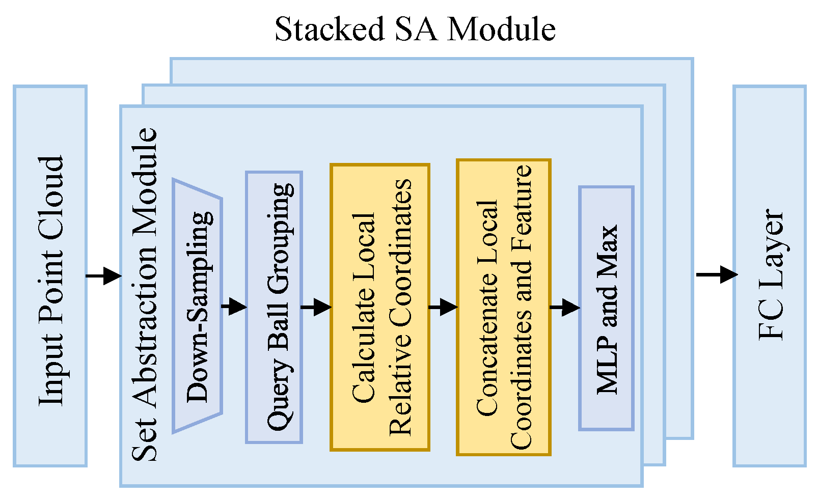
In this subsection, we propose an algorithm improving upon the typical PointNet++ backbone network. As shown in Figure 2, this model abstracts high-level features by stacking multiple Set Abstraction (SA) module values from bottom to top.
Consider a point set ( P = { ( x i , f i ) i = 1 , , N } , where x i R 3 represents the coordinates and f i R d represents the features). In the SA module, local feature extraction is achieved through downsampling, grouping, and feature aggregation, and the result is fed as input to the next layer. First, M center points are selected via sampling.
C = { c j } j = 1 M P , M < N
Subsequently, a local neighborhood is constructed around each center point ( c j ) using a k-Nearest Neighbors (k-NN) query.
N k ( c j ) = p p k - NN ( c j ) , k N +
This step outputs M local point groups ( N j j = 1 M ).
Finally, PointNet is applied independently to each N j to extract local features.
f j = γ MAX x i N j h f i , x i c j
where h ( · ) denotes a shared MLP that encodes point features and relative positions ( x i c j ), MAX is a symmetric aggregation function (e.g., max pooling), and γ represents subsequent MLPs for further feature refinement. The final output is a new point set ( P = { ( c j , f j ) } j = 1 M ).
However, directly using point-cloud data as features makes PointNet++ sensitive to pose perturbations. To improve robustness, this paper constructs a rotation-invariant feature extraction method. In addition, KNN or ball-query grouping calculates the distance of the entire point cloud. When dealing with large-scale point clouds, distance calculation leads to ultra large-scale matrix calculation. Although the method based on SpConv avoids distance calculation, it does not suffer from rotation invariance. For this purpose, this article constructs a rotation-invariant recursive segmentation method.

3.2. Inspection Framework

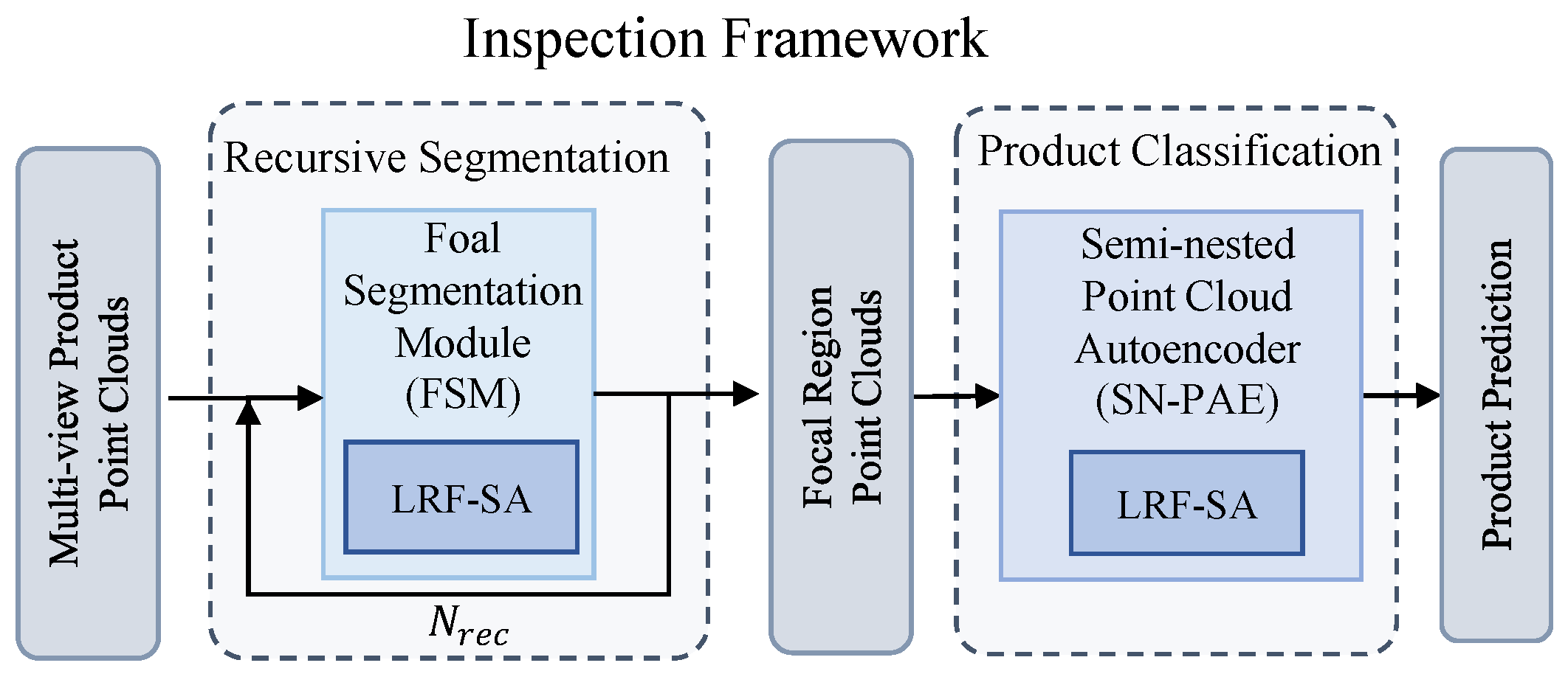
This inspection framework is specifically proposed for a closed production-line environment. As shown in Figure 3, the framework consists of two parts: recursive segmentation and one-class product classification. The recursive segmentation stage is achieved through N r e c iterative applications of the proposed FSM to the scanned 3D product point cloud, progressively isolating the fixed detection area. Subsequently, a uniquely designed semi-nested point-cloud autoencoder model determines the presence of defects within this segmented region. As exemplified in 3D solder-joint defect detection, the fixed region typically contains multiple solder-joint instances. Furthermore, to achieve rotation-invariant feature extraction, we introduce the Local Reference Frame (LRF) and propose an LRF-SA module, which is utilized across various components of the framework.

3.3. Recursive Segmentation Method

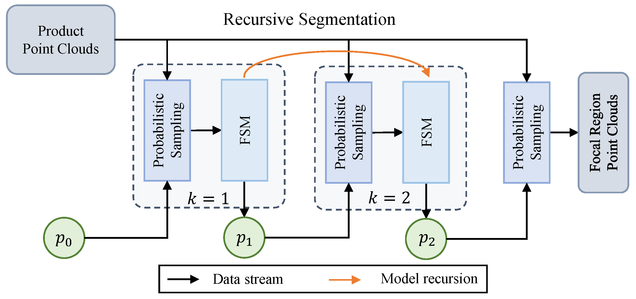
The details of the recursive segmentation method are shown in Figure 4. In contrast with baseline models for usual object detection or instance segmentation, recursive segmentation is proposed to achieve segmentation of fixed regions, where the key idea is to recursively focus the focal region using downsampled low-resolution data. As shown in Figure 4, when k = 1 , given an input point cloud ( P 0 R 3 ) with N 0 points and an initialized sampling probability of p 0 , we can obtain point cloud P 1 with N 1 points after probability sampling, which is mathematically described is as follows.
N k = E ( p k 1 ) = i = 1 i = N k 1 p k 1 i
where N k is the expectation of p k 1 . The N 0 elements of p 0 are initialized to 1.0 .
Next, we set the points in focal areas as foreground points with a 1.0 label, and other points are labeled as background points ( 0.0 ). Then, a Focal Segmentation Module (FSM, F f s m ) is proposed to calculate the prediction ( p 1 ) of input datum P 1 . At last, we perform probabilistic sampling in the next recursion. The mathematical description of recursion is expressed as follows.
p k = F f s m ( D ( P k 1 , p k 1 ) )
where F f s m is the FSM and D ( P k 1 , p k 1 ) refers to probability sampling P k 1 based on p k 1 .
During the recursive segmentation process, the FSM utilizes only a small number of skeleton points at each step. Since the number of predicted point clouds within the focal area of a foreground point is initially insufficient, multiple recursive iterations are required. In each new recursion, the sampling probability is derived from the previous FSM output, enabling the process to focus progressively on a subset of the prior segmentation. This iterative refinement gradually narrows the focus to a fixed area. Moreover, the reduction in the number of probabilistically sampled points with each recursion enhances the prediction accuracy of the FSM. It is particularly noteworthy that, due to the high similarity of production-line data, the N r e c recursive steps of the FSM effectively function to process N r e c distinct segmentation samples for the network.

3.4. Focal Segmentation Module

A Focal Segmentation Module (FSM) is proposed to achieve approximate segmentation of the focal area based on downsampled data at low resolution. As shown in Figure 5, an FSM contains 3 steps. First, a small amount of data ( P d ) is randomly down-sampled based on a large ratio with the same initial sampling probability for all points. Then, after segmentation on P d , we obtain the segmentation prediction ( y ^ d ) of the down-sampled point clouds. At last, by interpolating the K m nearest neighbors, we obtain indicative approximate predictions ( p k ) for all points at the kth recursion, where, usually, K m = 3 .
Focus segmentation is the core step of recursive segmentation. By utilizing only a small number of skeleton points in a single recursion, it significantly reduces the computational cost per step. This efficiency is pivotal; without the FSM, recursive segmentation using all data can be replaced by a general segmentation method such as PointNet++. In particular, it is easy to obtain downsampled data without the focal area point if the value of P d is too small. For instance, in our solder-joint inspection, we downsample only 1 k points from an original cloud of 300 k . To ensure a sufficient number of foreground points for effective segmentation, we construct the segmentation labels ( y d ) by designating all points within a radius ( r d ) of the focal areas as foreground. However, a large r d introduces redundancy into the probabilistically sampled data. To address this, we progressively decrease r d across the serially connected modules, thereby refining the segmentation and gradually focusing on the precise areas of interest. On the other hand, the inherent roughness of the downsampled, low-resolution point clouds makes it difficult for the FSM to segment fine structural details. Consequently, the FSM is particularly suited for controlled environments like our closed production line, where data exhibits high similarity.
The procedure of the proposed focal segmentation is summarized in Algorithm 1.
Algorithm 1 Focal Segmentation.
Input: 
The original scanned point clouds P o r i g i n ; Number of recursions N r e c ; The point cloud’s label y.
Output: 
Focal fixed-areas point cloud P N r e c .
  1:
Initial sampling probability p 0 = [ 1.0 ] N 0 ;
  2:
for  k = 1 , 2 , , N r e c  do.
  3:
      // Probability sampling.
  4:
       N k i = 1 | N k 1 | p k 1 i .
  5:
       P k ProbabilitySample ( P k 1 , p k 1 , N k ) .
  6:
      // Focal Segmentation Module.
  7:
       P d RandomDownsample ( P k , ratio ) // Large-ratio downsampling.
  8:
       y ^ d Segmentation ( P d ) .
  9:
      Label y d assignment with radius threshold r d .
10:
      // Interpolation using K nearest neighbors.
11:
       p k KNNInterpolate ( y ^ d , P d , P k , K m ) .
   return  P N r e c ProbabilitySample ( P k , p k , N k ) .

3.5. LRF-Based Set Abstraction

To improve the robustness of the model to pose changes, we introduce LRF-based rotation-invariant feature extraction to set abstraction in PointNet++ [28].
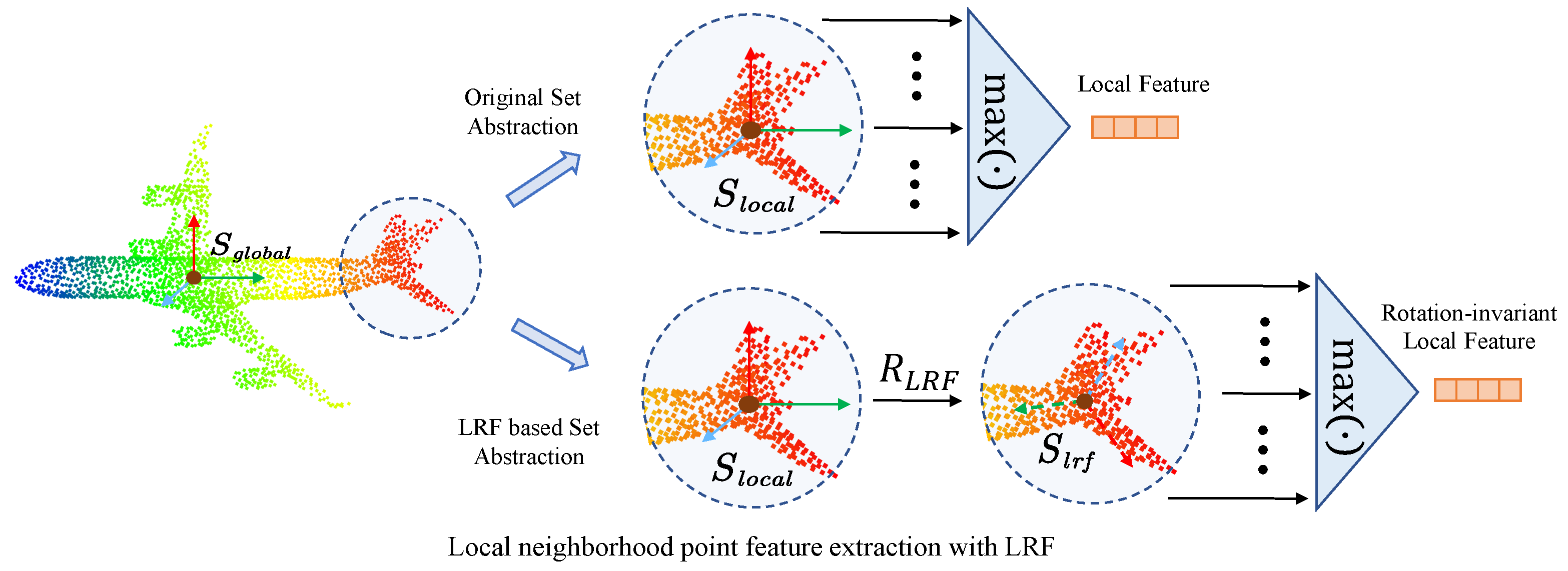
As shown in Figure 6, for a local point cloud, the existing rotation-sensitive methods generally directly use local relative point coordinates as features in the model like PointNet++ [28]. However, the coordinates ( P l o c a l R 3 ) in the local reference frame ( S l o c a l ) are sensitive to pose changes, resulting in poor robustness of such methods. To solve this problem, we construct a Local Reference Frame (LRF, S l r f ) for the local point cloud, an the point cloud coordinates P l r f R 3 under S l r f remain unchanged when the pose changes; thus, the model remains robust if we use P l r f instead of P l o c a l . The specific calculation process of LRF is expressed as follows.
First, the local neighborhood ( N ( p l ) ) is defined. The neighborhood can be determined using k-nearest neighbors (k-NN) or radius search. To ensure regular tensor computation, this paper adopts the KNN approach.
The covariance matrix ( C R 3 × 3 ) of the neighborhood point set is computed as follows:
C = 1 | N ( p l ) | q l N ( p l ) ( q l p l ¯ ) ( q l p l ¯ )
where p l ¯ = 1 | N ( p l ) | q l N ( p l ) q l is the centroid of the neighborhood.
Eigenvalue decomposition is performed on C :
C = V Λ V , Λ = diag ( λ 1 , λ 2 , λ 3 ) , λ 1 λ 2 λ 3
where eigenvectors v 1 , v 2 , and v 3 correspond to the principal directions. The sign is adjusted using the following rule:
z = sign ( v 3 · ( P l p l ) ) · v 3
The same method is used to determine x , and y is obtained via the cross product. Finally, the local reference frame is represented by the orthogonal matrix ( R L R F SO ( 3 ) ):
S l o c a l = R L R F = [ x , y , z ] st . R L R F R L R F = I
This matrix transforms the neighborhood points ( P l o c a l ) in local coordinates to local coordinates ( P l r f ):
P l r f = P l o c a l R L R F
As shown in Figure 6, the point cloud and features under the LRF are fused through a PointNet [28] network, and middle-level features are extracted for subsequent operations.
In summary, the cost required by focal segmentation is much smaller than the method that directly uses the whole raw data for detection, and the introduction of LRF improves the robustness of the FSM.

3.6. Semi-Nested Point Cloud Autoencoder

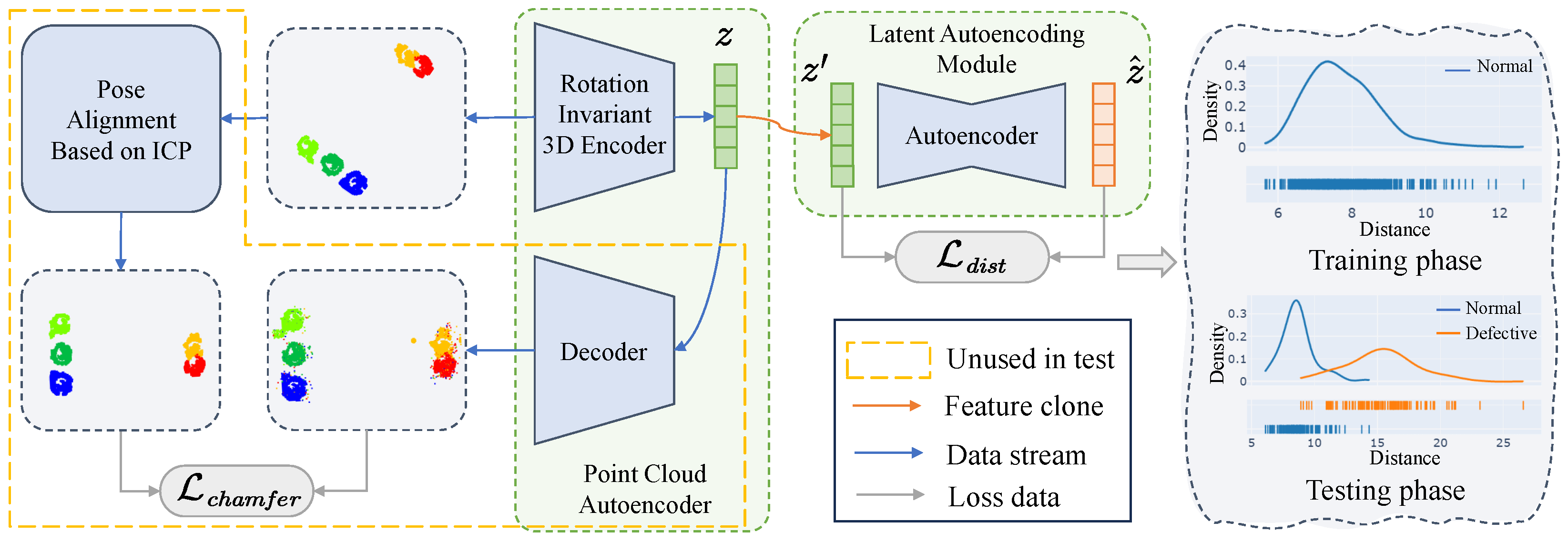
After segmenting the focal areas, a Semi-Nested Point Cloud Autoencoder (SN-PAE) is proposed to realize the judgment of the areas. It should be noted that some of the contents of SN-PAE were reported in a conference paper [40]. A schematic diagram of the proposed SN-PAE is shown in Figure 7. SN-PAE mainly includes two submodules: an Rotation-Invariant Point Cloud Autoencoder (RI-PAE) and a Latent Autoencoding Module (LAM).
The RI-PAE includes two modules: a rotation-invariant 3D encoder with LRF-based set abstraction and a decoder. The decoder in RI-PAE is consistent with the deep autoencoder. It performs nonlinear transformation and dimensionality enhancement on the latent variable. The output is finally transformed to a point cloud with a shape of [ N t , 3 ] , where N t is the point number of the target point cloud. This point cloud is used for subsequent chamfer distance measurement. The latent variable of the autoencoder is the output of the rotation-invariant 3D encoder; thus, the learned latent variable is rotation-invariant. The semi-nested LAM is a deep autoencoding whose input and output dimensions are consistent with the RI-PAE latent variable (z). The measurement method of the LAM uses Euclidean distance.
Since the sample data input and modules used in training and testing are different, the two phases are described independently. In the training phase, the input unaligned normal sample point cloud ( P n o r o r i ) is first registered with the manual pre-built template ( P t e m p l a t e ) based on the point-to-plan Iterative Closest Point algorithm [7] ( I C P ), and the rotation matrix ( R i c p ) is calculated. We use the unaligned point cloud ( P n o r o r i ) and rotation matrix ( R i c p ) to calculate the aligned point cloud ( P n o r a l i g n ), whose pose is consistently with the template. The mathematical description is shown below:
R i c p = I C P ( P n o r o r i , P t e m p l a t e )
P n o r a l i g n = P n o r o r i R i c p
Then, we take this aligned point cloud ( P n o r a l i g n ) as the generation target and generate a point cloud based on RI-PAE to approximate the target.
At the same time, we semi-nest the LAM in the RI-PAE. By cloning the latent variable (z) of the RI-PAE as the latent variable generation target ( z ), we input it into the LAM and generate a vector ( z ^ ) to approximate z . After training, the latent variable (z) learned by the RI-PAE is a descriptive rotation-invariant quantity. At the same time, the LAM finally learns the true distribution of the input latent variable ( z ) and can generate it well.
In the testing phase, we input samples ( P o r i ). The defective samples generate a special latent variable ( z d e f ). Compared with the latent variable transformed by the normal samples ( z n o r ), z d e f should be outliers in the z n o r distribution. Therefore, the distance between z h a t generated by LAM and z cloned from RI-PAE can be measured to directly determine whether the input sample point cloud ( P o r i ) is defective. Therefore, the decoder work of RI-PAE and a point cloud sample-based chamfer distance metric is not required at test time.
It should be emphasized that due to the unique network structure design, it is unnecessary to compute the chamfer distance between point clouds during testing. Since the latent variable (z) learned by the RI-PAE encoder is rotation-invariant, the relative poses of the input and reconstructed samples become irrelevant. This decoupling renders chamfer distance comparisons between input and output samples meaningless. Instead, the additionally designed Latent Analysis Module (LAM) transforms the similarity measure from chamfer distance in 3D space to Euclidean distance in the latent space. Through this strategy, we effectively mitigate the negative impact of pose variation and maintain model robustness. On the other hand, unlike the dataset that employs only a single rotation matrix obtained through manual prior registration, the heuristic ICP algorithm in practical registration scenarios produces fluctuating rotation matrices across multiple registrations. This leads to unstable pose estimates and occasional registration failures. Such inherent instability further undermines the robustness of the RI-PAE model against pose perturbations.
The procedure of the proposed SN-PAE is summarized in Algorithm 2.
Algorithm 2 Semi-Nested Point Cloud Autoencoder (SN-PAE).
Input: 
Point cloud obtained from focus segmentation P s e g ; Template point cloud P t e m p l a t e ; Preset threshold t h d .
Output: 
Product quality assessment N o r m a l / D e f e c t i v e .
  1:
Initial Rotation invariant encoder E R I , Rotation invariant decoder D R I , latent variable encoder E L , latent variable decoder D L
  2:
z E R I ( P s e g )
  3:
z Clone ( z )
  4:
z ^ D L ( E L ( z ) )
  5:
L L A M EuclideanDistance ( z ^ , z )
  6:
if Training then
  7:
       R i c p ICP ( P s e g , P t e m p l a t e )
  8:
       P a l i g n P s e g · R i c p
  9:
       P ^ a l i g n D R I ( z )
10:
       L R I ChamferDistance ( P ^ a l i g n , P a l i g n )
11:
       L t o t a l L R I + L L A M
12:
      Update parameters of E R I , D R I , E L , D L
13:
else
14:
      if  s c o r e > t h d  then
15:
             y 1 // Defective
16:
      else
17:
             y 0 // Normal

3.7. Loss

The total target loss of the proposed framework is the sum of the recursive segmentation and classification losses. The mathematical expression is presented as follows.
L = i = 1 i = N R e c L R e c S e g i + L C l s ,
where the first term is the sum of the losses of the N R e c FSMs and L C l s is the SN-PAE loss for classification. The recursive segmentation loss in every recursion is cross-entropy loss, and the loss of SN-PAE includes two parts: the chamfer distance loss of RI-PAE and the Euclidean distance loss of the LAM. The mathematical expression is presented as follows.
L c h a m f e r S 1 , S 2 = 1 S 1 x S 1 min y S 2 | | x y | | 2 2 + 1 S 2 y S 2 min x S 1 | | y x | | 2 2 ,
where S 1 and S 2 represent the target point cloud and the generated point cloud and x and y refer to the point coordinates in S 1 and S 2 .
L d i s t Z 1 , Z 2 = 1 N i = 1 i = N Z 1 i Z 2 i 2 ,
where Z 1 and Z 2 represent the target latent variable vector and the generated latent variable vector, Z 1 i and Z 1 i represent the elements of vectors Z 1 and Z 2 , and N is the vector dimension.
L C l s = L c h a m f e r + η L d i s t
where η is an artificially set weight coefficient. Since the modulus of the vector is small, in this article, we set η = 5.0 to speed up the training of the LAM.
Overall, we carefully consider the particularity of the production-line environment and propose an inspection framework for reliable and robust high-quality 3D quality inspection.

4. Experiments and Analysis

Several sets of experiments are implemented to evaluate the performance of the proposed framework. This section includes the following items.
(1)
Several datasets are built.
(2)
The experimental setup and metrics are introduced.
(3)
The experimental results are explained in detail.

4.1. Datasets

We constructed three datasets—namely, DHU-RADER1000-ICP, DHU-PAD1000-ICP, and ModelNet40-Toy-AC. The former two datasets were obtained from the production-line data, and ModelNet40-Toy-AC was extracted from the public ModelNet40 dataset [6].
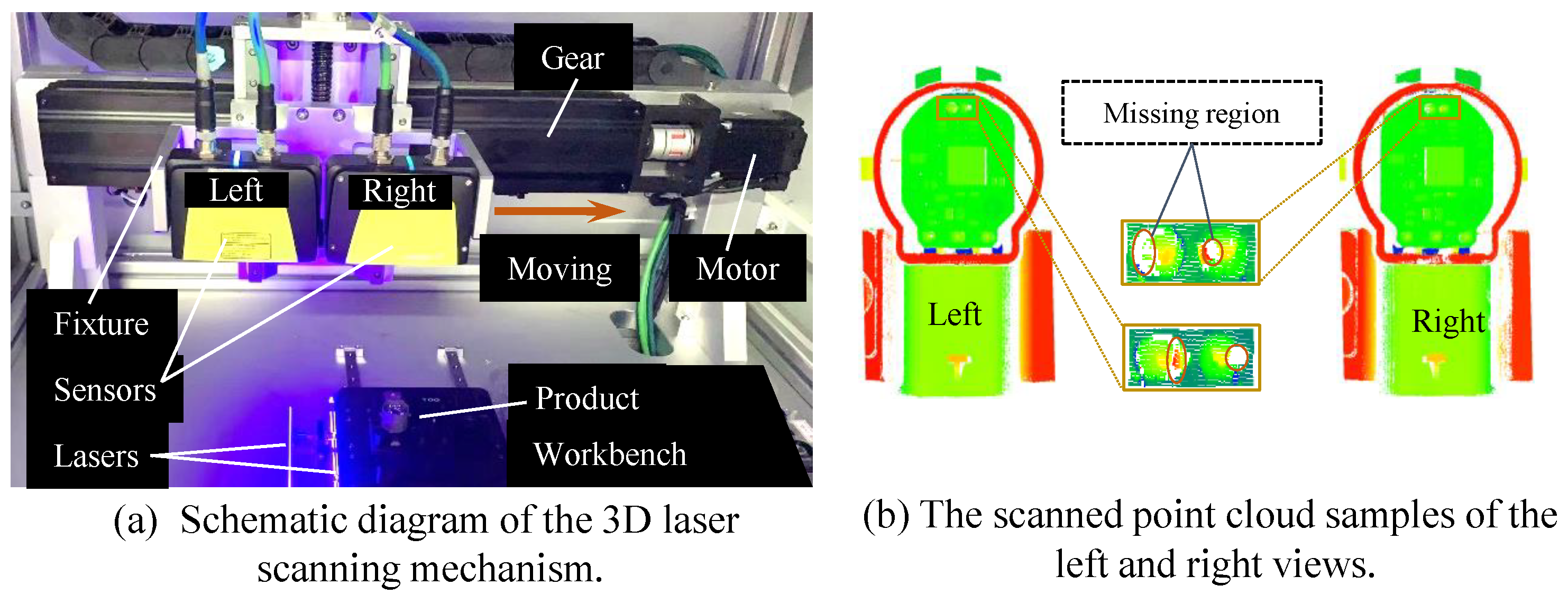
The 3D scanning system is shown in Figure 8a. We use the ECCO95 model and build a set of sensors using a back-to-back approach. Through the worm gear hinged with the motor, the laser sensors realize linear reciprocating motion. During movement, all scanned data frames are collected and integrated into a point cloud for subsequent detection and dataset construction. As shown in Figure 8b, we use the back-to-back sensors to obtain point clouds of opposing perspectives to ensure the completeness of the data. The left- and right-view data can complement each other to obtain complete solder-joint data. In the closed production-line environment, the samples in the dataset are highly similar, and the overall samples are basically the same, with only minor differences in the solder-joint area.
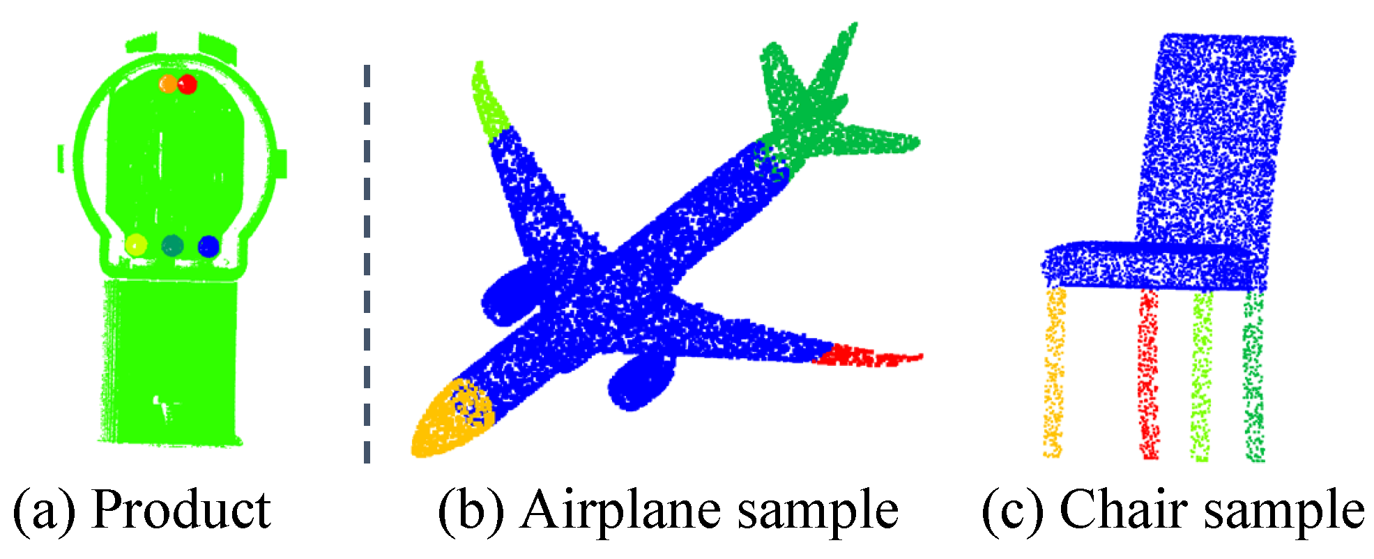
DHU-RADER1000-ICP is constructed based on the scanned data. The number of points in each view is about 300 k , and the number of points of each solder joint is about 1 k . A sample with 5 solder joint areas is shown in Figure 9a. The dataset partition of the constructed dataset for segmentation partition is shown in Table 1, and classification is shown in Table 2.
In order to verify the generalization ability of the proposed method, ModelNet40-Toy-AC is constructed from ModelNet40 [6] data. Since the production-line data has a high degree of similarity, in order to replicate data similar to the actual production-line characteristics, we extract some samples from the airplane and chair classes. We set four regions of interest for each class, and two samples are shown in Figure 9. The dataset partition of the constructed dataset for segmentation partition is shown in Table 1.
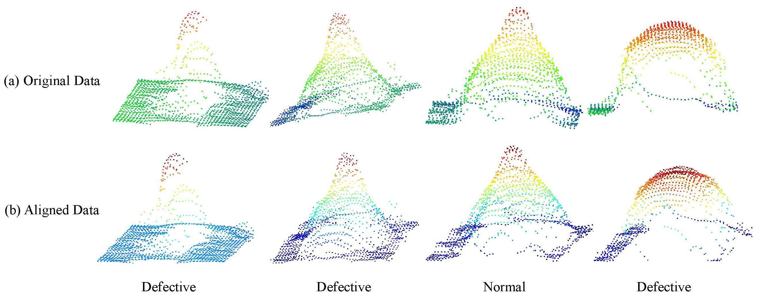
We also build a solder-joint point-cloud dataset named DHU-PAD1000-ICP from laser-scanned data, some samples of which are shown in Figure 10. As shown in Figure 10a, the poses of these original solder joints are inconsistent due to assembly errors. To facilitate training, we set the reference pose using a manual template during preprocessing and calculate the rotation matrix using the point-to-plan ICP algorithm. The aligned sample is shown in Figure 10b. In particular, the appearance of some defective samples is very close to that of normal samples, requiring the model to have detailed feature discrimination capabilities. The dataset partition of the constructed dataset for classification is shown in Table 2. In the one-class classification stage, only normal samples are used during training.

4.2. Experimental Setup

To verify the effectiveness of the proposed framework, multiple sets of experiments are implemented, including experiments on the segmentation phase, comparing the product classification loss, and evaluating quantitative robustness. Some quantitative metrics are introduced to evaluate the performance of the method. In the recursive segmentation stage, we evaluate the defective-region segmentation performance using the mean Intersection overUnion (IoU) of foreground points in the fixed areas. In the one-class classification stage, we hope to set a reasonable threshold ( t h d ) to ensure that all defective samples are detected out and, at the same time, the recall rate R e c a l l ( @ t h d ) of normal samples is as high as possible to reduce the false detection rate. Therefore, we use the minimum distance ( d d e f m i n ) between defective products and the recall rate ( R e c a l l ( @ d d e f m i n ) ) of normal samples at the minimum distance as an indicator. The larger the minimum distance is, the larger the optional range of thresholds is, and it is easier to find a suitable threshold. A higher recall rate means a lower false detection rate, less work required for manual inspection, and better model performance.
The hardware mainly includes a computer with two Nvidia GeForce RTX 6000 GPUs and 128 GB RAM, and the proposed method is developed based on the PyTorch 1.12 deep learning library. Unless otherwise stated, some experimental hyperparameters for training are set as follows. Optimization is performed with an Adam optimizer. The initial learning rate is set to 0.001, the weight decay is set to 0.0001, the momentum is 0.9, and the training batch size is set to 16. Specifically, we used Open3D and CloudCompare for 3D point-cloud visualization and processing and Origin for data analysis and graph plotting.

4.3. Experimental Results

In this subsection, we describe and analyze the results of the multiple implemented sets of experiments in turn.

4.3.1. Segmentation-Stage Experiments

In DHU-RADER1000-ICP, fixed-area data accounts for 1∼2% of the overall data, and we set each FSM to segment about 10% of the foreground data so that N R e c is set to 2 to obtain relatively accurate detection-area data for the fixed areas. In ModelNet40-Toy-AC, the foreground data accounts for about 5∼10%; thus, setting N R e c = 2 is enough.
The experimental results of the segmentation stage are shown in Table 3 and Table 4. In Table 3, we validate the proposed method on two datasets and compare it with the classic PointNet++. The segmentation IoU of the proposed method is similar to that of existing methods, and the performance gap between the proposed method and RandLANet and RIConv++ on the two datasets is less than 2%, but it is better than PointNet++ based on LRF. Specifically, the accuracy of the proposed method is nearly 5 % greater than that of PointNet++ on ModelNet40-Toy-AC. As shown in Table 4, the cost of the proposed framework is much less than that of PointNet++. According to the comparison results, although RandLANet achieved the best performance, it has the highest computational cost. In contrast, the proposed recursive segmentation uses fewer layers and feature channels because it only needs to segment the coarse point-cloud structure. Therefore, the parameter count of the recursive segmentation network is about 12 % of that of PointNet++. When the number of points is 10 k, the costs of the proposed method and PointNet++ are similar. However, when the point number reaches 300 k, the memory cost of the proposed framework is 8 % of that of PointNet++, the time cost is about 2.5 % of that of PointNet++, and the calculation amount is only 3.3 % of that of PointNet++. With the expansion of the point-cloud scale, our method shows huge advantages in terms of calculation account, time cost, and memory cost. Specifically, the network structure of PointNet++ does not add layers as the number of points increases, so PointNet++ is only used as a reference for the cost comparison here.
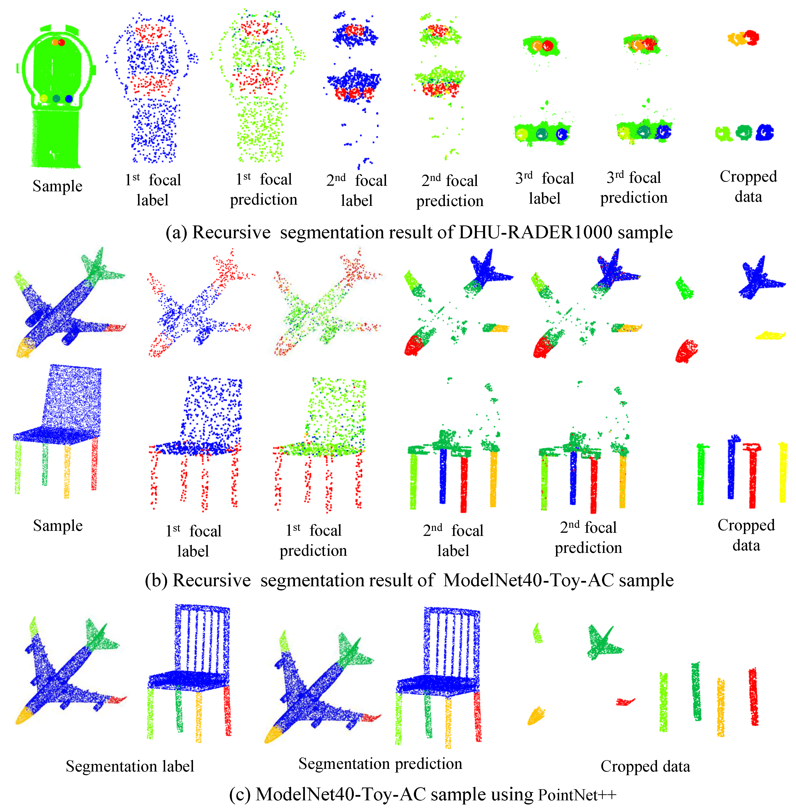
For intuition, we visualize the segmentation results of the segmentation stage. As shown in Figure 11, a rough segmentation prediction can be learned based on a small number of downsampled points, and multiple FSMs can efficiently propose invalid point clouds outside the fixed-area regions. In particular, the details of the segmented instances are basically preserved, and point redundancy of about 1 time brings about less than a 0.5 times increase in scale.

4.3.2. Classification-Stage Experiments

In one-class classification-stage experiments, we evaluate the model performance from two perspectives: comparison with existing advanced methods and comparison under different pose settings. Among them, different pose conditions are set to evaluate the robustness of the model’s point-cloud reconstruction to target point-cloud pose perturbations. The settings mainly include A l i g n e d / A l i g n e d , A l i g n e d / U n a l i g n e d , and A u g m e n t e d / U n a l i g n e d . A l i g n e d means that the sample has been aligned, U n a l i g n e d represents the original sample, and A u g m e n t e d refers to randomly rotation of the original data within a suitable range during training. The left side of / is the training setting, and the right side is the testing setting. In addition, the average Standard Deviation (SD) of 20 tests conducted on each sample is calculated. The experimental results are shown in Table 5.
We compare multiple models on the DHU-PAD1000-ICP dataset, including OCCNN [20], FoldingNet [37], TargetNet [39], and the proposed SN-PAE. Unlike strongly supervised classifiers and standard autoencoders, OCCNN generates defective samples by introducing perturbations like Gaussian noise, using PointNet++ as its backbone in our implementation. As shown in Table 5, OCCNN cannot effectively distinguish whether samples have defects under all pose conditions. We suggest that OCCNN learns an unrealistic decision boundary due to its inability to simulate the complex structural and semantic information characteristic of real defects. Autoencoder-based methods, including FoldingNet, TearingNet, and our proposed SN-PAE, all achieve strong defect detection performance on pose-aligned samples. Their similar recall rates for normal samples indicate effective learning of detailed solder-joint structures. However, FoldingNet and TearingNet show significant performance degradation when processing unaligned samples, with recall rates dropping by nearly 50% compared to their performance on aligned data. Even with data augmentation during training, their recall rates remain substantially lower than those of SN-PAE. In contrast, our SN-PAE maintains robust performance across varying pose conditions. It outperforms existing methods by more than 20% on unaligned samples. However, the recall rate of SN-PAE is approximately 10% lower than that of the first two methods on aligned samples. This performance trade-off is introduced by the architectural modifications in SN-PAE, which employs a semi-nested autoencoder and replaces the chamfer distance metric of PAE with a Euclidean distance metric in the semi-nested LAM. We attribute this performance trade-off to the inherent properties of autoencoders. Since an autoencoder obtains a low-dimensional latent variable through compression [35], a distributional discrepancy arises between the source data and the latent variable (z). We propose that it is this distributional discrepancy that leads to the performance degradation. Consequently, future work should explore the imposition of additional constraints on the latent space of RI-PAE. The objective is to increase the discriminativity of the latent distribution, thereby improving the separation between normal and defective samples.
As shown in Table 5, similar trends are observed on the DHU-RADER1000-ICP dataset. OCCNN is excluded from comparison due to its consistently poor performance. The proposed SN-PAE demonstrates stable performance across 20 tests, as evidenced by robust standard deviation (SD) values. It should be emphasized that the SD metric is particularly important for real-world applications. In practice, the decision threshold is typically set based on the minimum score of defective samples ( d d e f m i n ), then reduced by several standard deviations to enhance detection reliability. Assuming a normal distribution of prediction results, this multiplier is conventionally set to 3. Engineers need to adjust it according to actual working conditions.
The results of SN-PAE in ablation experiments on the DHU-RADER1000-ICP and DHU-PAD1000-ICP datasets are shown in Table 6. PAE is obtained by removing LRF and LAM from SN-PAE. Without LRF, SN-PAE cannot be robust to unaligned samples and has a larger SD on DHU-RADER1000-ICP. After using LRF, PAE achieves robustness to unaligned samples. However, it should be emphasized that although the LRF-based PAE achieves the best recall, it does not take into account the instability of the heuristic ICP registration. SN-PAE uses the latent Euclidean distance metric of the LAM to replace the unstable reconstruction error. Although it causes certain performance degradation, it effectively improves the robustness of the detection algorithm.
In addition, we construct two experiments to evaluate the robustness of the proposed framework to pose variations brought about by quantized rotations. Quantified rotation robustness test results are shown in Figure 12. We tested the performance of the pre-trained model once by rotating the dataset sample at a fixed angle on any axis and performed multiple tests. Obviously, the proposed framework introduced with LRF is robust to pose changes, and the opposite is true when LRF is not used. This demonstrates the effectiveness of LRF.
In summary, by using low-resolution data and introducing rotation-invariant feature extraction, the proposed recursive segmentation method achieves robust focal-region segmentation with less memory cost, time cost, and computation cost. In the classification stage, through additional latent autoencoding, the measurement method is changed from the chamfer distance between point-cloud samples to the rotation-invariant latent variable distance, which effectively avoids the adverse effects of point-cloud pose disturbance and achieves efficient and robust one-class learning for 3D point-cloud objects. The method is evaluated on samples with significantly varying shapes and scales, including objects (e.g., entire products, airplanes, and chairs) for segmentation and regions (e.g., single solder joints and multi-joint areas) for classification. Experimental results validate its effectiveness, suggesting a considerable degree of universality.

5. Conclusions and Future Work

We studied 3D fixed-area defect detection in industrial production lines, taking into account the uniqueness of the production-line scenario and the preference of industrial inspection for classification metrics. In this paper, we constructed a progressive segmentation method based on point-cloud deep learning and realized high-resolution fixed-area detection by using downsampled data. Moreover, we ensured the robustness of the method to pose changes by introducing LRF-based rotation-invariant feature extraction. On the other hand, we approached the requirement of zero false detections in industrial inspection by manipulating the model prediction distribution. The proposed SN-PAE first uses a rotation-invariant point-cloud autoencoder to convert the point-cloud chamfer distance-based measurement into a rotation-invariant latent variable measurement, thereby effectively improving the 3D point-cloud autoencoder’s robustness to target point-cloud pose perturbations. Finally, a group of experiments was implemented on two constructed datasets, and the results show the effectiveness of the proposed method.
The idea of this method can be easily transferred to other task scenarios, especially other production-line tasks with an unfixed pose, for example, the shape inspection of small industrial products such as buttons and hardware in production lines. However, the proposed method is currently limited to fixed-area detection, and more efficient segmentation methods need to be developed to cope with defect detection with non-fixed positions. Moreover, the proposed method currently still requires the addition of manual templates during training, and a complete end-to-end approach will be the subject of future work.

Author Contributions

Conceptualization and supervision, K.H.; methodology and writing, H.L.; investigation and validation, B.W. and X.-s.T.; hardware and data preparation, T.Z. and P.Z. All authors have read and agreed to the published version of the manuscript.

Funding

This work was supported in part by the Fundamental Research Funds for the Central Universities and Graduate Student Innovation Fund of Donghua University (CUSF-DH-D-2021055).

Data Availability Statement

The data presented in this study are available on request from the corresponding author due to legal reasons.

Acknowledgments

This article is a revised and expanded version of a paper entitled A Semi-Nested Point Cloud Autoencoder for Solder Joint Inspection, which was presented at the International Symposium on Autonomous Systems (ISAS) on 15 March 2024, in Chongqing, China.

Conflicts of Interest

The authors declare no conflicts of interest.

Abbreviations

The following abbreviations are used in this manuscript:
LRFLocal Reference Frame
FSMFocal Segmentation Module
SN-PAESemi-Nested Point Cloud Autoencoder
LAMLatent Autoencoding Module

References

  1. Ko, J.H.; Yin, C. A Review of Artificial Intelligence Application for Machining Surface Quality Prediction: From Key Factors to Model Development. J. Intell. Manuf. 2025. [Google Scholar] [CrossRef]
  2. Guo, Y.; Wang, H.; Hu, Q.; Liu, H.; Liu, L.; Bennamoun, M. Deep Learning for 3d Point Clouds: A Survey. IEEE Trans. Pattern Anal. Mach. Intell. 2021, 43, 4338–4364. [Google Scholar] [CrossRef]
  3. Zhang, J.; Zhou, Z.; Sun, J. Center-Aware Instance Segmentation for Close Objects in Industrial 3-D Point Cloud Scenes. IEEE Trans. Ind. Inform. 2024, 20, 2812–2821. [Google Scholar] [CrossRef]
  4. Wei, C.; Bao, Y.; Zheng, C.; Ji, Z. AMFNet: Aggregated Multi-Level Feature Interaction Fusion Network for Defect Detection on Steel Surfaces. J. Intell. Manuf. 2025. [Google Scholar] [CrossRef]
  5. Saberironaghi, A.; Ren, J.; El-Gindy, M. Defect Detection Methods for Industrial Products Using Deep Learning Techniques: A Review. Algorithms 2023, 16, 95. [Google Scholar] [CrossRef]
  6. Wu, Z.; Song, S.; Khosla, A.; Yu, F.; Zhang, L.; Tang, X.; Xiao, J. 3d Shapenets: A Deep Representation for Volumetric Shapes. In Proceedings of the IEEE Conference on Computer Vision and Pattern Recognition, Boston, MA, USA, 7–12 June 2015; pp. 1912–1920. [Google Scholar]
  7. Chen, Y.; Medioni, G. Object Modelling by Registration of Multiple Range Images. Image Vis. Comput. 1992, 10, 145–155. [Google Scholar] [CrossRef]
  8. Li, H.; Hao, K.; Wei, B.; Tang, X.s.; Hu, Q. A Reliable Solder Joint Inspection Method Based on a Light-Weight Point Cloud Network and Modulated Loss. Neurocomputing 2022, 488, 315–327. [Google Scholar] [CrossRef]
  9. Hu, Q.; Hao, K.; Wei, B.; Li, H. An Efficient Solder Joint Defects Method for 3D Point Clouds with Double-Flow Region Attention Network. Adv. Eng. Inform. 2022, 52, 101608. [Google Scholar] [CrossRef]
  10. Zhang, Z.; Hua, B.S.; Yeung, S.K. RIConv++: Effective Rotation Invariant Convolutions for 3D Point Clouds Deep Learning. Int. J. Comput. Vis. 2022, 130, 1228–1243. [Google Scholar] [CrossRef]
  11. Armeni, I.; Sener, O.; Zamir, A.R.; Jiang, H.; Brilakis, I.; Fischer, M.; Savarese, S. 3D Semantic Parsing of Large-Scale Indoor Spaces. In Proceedings of the 2016 IEEE Conference on Computer Vision and Pattern Recognition (CVPR), Las Vegas, NV, USA, 27–30 June 2016; pp. 1534–1543. [Google Scholar] [CrossRef]
  12. Zhang, Z.; Gao, P.; Peng, S.; Duan, C.; Zhang, P. Enhanced Point Feature Network for Point Cloud Salient Object Detection. IEEE Signal Process. Lett. 2023, 30, 1617–1621. [Google Scholar] [CrossRef]
  13. Vu, T.; Kim, K.; Luu, T.M.; Nguyen, T.; Yoo, C.D. Softgroup for 3d Instance Segmentation on Point Clouds. In Proceedings of the IEEE/CVF Conference on Computer Vision and Pattern Recognition, New Orleans, LA, USA, 18–24 June 2022; pp. 2708–2717. [Google Scholar]
  14. Wei, B.; Hao, K.; Gao, L.; Tang, X.S. Bioinspired Visual-Integrated Model for Multilabel Classification of Textile Defect Images. IEEE Trans. Cogn. Dev. Syst. 2021, 13, 503–513. [Google Scholar] [CrossRef]
  15. Wang, D.; Su, S.; Lu, X. RSD-Diff: Boundary-Frequency Feature-Enhanced Rail Surface Defect Inspection with Diffusion-Based Transformer Decoder. In Proceedings of the 2024 10th International Conference on Systems and Informatics (ICSAI), Shanghai, China, 14–16 December 2024; pp. 1–6. [Google Scholar] [CrossRef]
  16. Qin, T.; Chen, D.; Xiang, J.; Tian, Z. SP-YOLO: A Model for Detecting Solder Paste Printing-Defect in PCB. In Proceedings of the 2025 8th International Conference on Advanced Algorithms and Control Engineering (ICAACE), Shanghai, China, 21–23 March 2025; pp. 1251–1254. [Google Scholar] [CrossRef]
  17. Reddy, V.V.; Ume, I.C.; Williamson, J.; Sitaraman, S.K. Evaluation of the Quality of BGA Solder Balls in FCBGA Packages Subjected to Thermal Cycling Reliability Test Using Laser Ultrasonic Inspection Technique. IEEE Trans. Compon. Packag. Manuf. Technol. 2021, 11, 589–597. [Google Scholar] [CrossRef]
  18. Yan, H.; Zhang, H.; Gao, F. Transforming PCB Solder Joint Detection with Deep Learning Empowered X-ray Nondestructive Testing. In Proceedings of the 2024 IEEE Far East NDT New Technology & Application Forum (FENDT), Zhongshan, China, 24–27 June 2024; pp. 26–30. [Google Scholar] [CrossRef]
  19. Dai, W.; Mujeeb, A.; Erdt, M.; Sourin, A. Soldering Defect Detection in Automatic Optical Inspection. Adv. Eng. Inform. 2020, 43, 101004. [Google Scholar] [CrossRef]
  20. Oza, P.; Patel, V.M. One-Class Convolutional Neural Network. IEEE Signal Process. Lett. 2019, 26, 277–281. [Google Scholar] [CrossRef]
  21. Ruff, L.; Vandermeulen, R.; Goernitz, N.; Deecke, L.; Siddiqui, S.A.; Binder, A.; Müller, E.; Kloft, M. Deep One-Class Classification. Proc. Mach. Learn. Res. 2018, 80, 4393–4402. [Google Scholar]
  22. Perera, P.; Nallapati, R.; Xiang, B. Ocgan: One-Class Novelty Detection Using Gans with Constrained Latent Representations. In Proceedings of the IEEE/CVF Conference on Computer Vision and Pattern Recognition, Long Beach, CA, USA, 15–20 June 2019; pp. 2898–2906. [Google Scholar]
  23. Sabokrou, M.; Khalooei, M.; Fathy, M.; Adeli, E. Adversarially Learned One-Class Classifier for Novelty Detection. In Proceedings of the IEEE Conference on Computer Vision and Pattern Recognition, Salt Lake City, UT, USA, 18–23 June 2018; pp. 3379–3388. [Google Scholar]
  24. Vincent, P.; Larochelle, H.; Bengio, Y.; Manzagol, P.A. Extracting and Composing Robust Features with Denoising Autoencoders. In Proceedings of the 25th International Conference on Machine Learning—ICML’08, Helsinki, Finland, 5–9 July 2008; pp. 1096–1103. [Google Scholar] [CrossRef]
  25. Masana, M.; Ruiz, I.; Serrat, J.; van de Weijer, J.; Lopez, A.M. Metric Learning for Novelty and Anomaly Detection. arXiv 2018, arXiv:1808.05492. [Google Scholar] [CrossRef]
  26. Perera, P.; Oza, P.; Patel, V.M. One-Class Classification: A Survey. arXiv 2021, arXiv:2101.03064. [Google Scholar] [CrossRef]
  27. Qi, C.R.; Su, H.; Mo, K.; Guibas, L.J. Pointnet: Deep Learning on Point Sets for 3d Classification and Segmentation. In Proceedings of the IEEE Conference on Computer Vision and Pattern Recognition, Honolulu, HI, USA, 21–26 July 2017; pp. 652–660. [Google Scholar]
  28. Qi, C.R.; Yi, L.; Su, H.; Guibas, L.J. Pointnet++: Deep Hierarchical Feature Learning on Point Sets in a Metric Space. In Proceedings of the Advances in Neural Information Processing Systems, Long Beach, CA, USA, 4–9 December 2017; pp. 5105–5114. [Google Scholar]
  29. Wang, Y.; Ye, T.; Cao, L.; Huang, W.; Sun, F.; He, F.; Tao, D. Bridged Transformer for Vision and Point Cloud 3d Object Detection. In Proceedings of the IEEE/CVF Conference on Computer Vision and Pattern Recognition, New Orleans, LA, USA, 18–24 June 2022; pp. 12114–12123. [Google Scholar]
  30. Zhang, Q.; Hou, J. PointVST: Self-Supervised Pre-Training for 3D Point Clouds via View-Specific Point-to-Image Translation. IEEE Trans. Vis. Comput. Graph. 2024, 30, 6900–6912. [Google Scholar] [CrossRef]
  31. Zhang, C.; Wan, H.; Shen, X.; Wu, Z. Pvt: Point-Voxel Transformer for Point Cloud Learning. Int. J. Intell. Syst. 2022, 37, 11985–12008. [Google Scholar] [CrossRef]
  32. Gojcic, Z.; Zhou, C.; Wegner, J.D.; Wieser, A. The Perfect Match: 3d Point Cloud Matching with Smoothed Densities. In Proceedings of the IEEE/CVF Conference on Computer Vision and Pattern Recognition, Long Beach, CA, USA, 15–20 June 2019; pp. 5545–5554. [Google Scholar]
  33. Deng, H.; Birdal, T.; Ilic, S. PPFNet: Global Context Aware Local Features for Robust 3D Point Matching. In Proceedings of the 2018 IEEE/CVF Conference on Computer Vision and Pattern Recognition, Salt Lake City, UT, USA, 18–23 June 2018; pp. 195–205. [Google Scholar] [CrossRef]
  34. Xu, M.; Ding, R.; Zhao, H.; Qi, X. Paconv: Position Adaptive Convolution with Dynamic Kernel Assembling on Point Clouds. In Proceedings of the IEEE/CVF Conference on Computer Vision and Pattern Recognition, Nashville, TN, USA, 20–25 June 2021; pp. 3173–3182. [Google Scholar]
  35. Hinton, G.E.; Salakhutdinov, R.R. Reducing the Dimensionality of Data with Neural Networks. Science 2006, 313, 504–507. [Google Scholar] [CrossRef]
  36. Achlioptas, P.; Diamanti, O.; Mitliagkas, I.; Guibas, L. Learning Representations and Generative Models for 3d Point Clouds. Proc. Mach. Learn. Res. 2018, 80, 40–49. [Google Scholar]
  37. Yang, Y.; Feng, C.; Shen, Y.; Tian, D. Foldingnet: Point Cloud Auto-Encoder via Deep Grid Deformation. In Proceedings of the IEEE Conference on Computer Vision and Pattern Recognition, Salt Lake City, UT, USA, 18–22 June 2018; pp. 206–215. [Google Scholar]
  38. Chen, S.; Duan, C.; Yang, Y.; Li, D.; Feng, C.; Tian, D. Deep Unsupervised Learning of 3D Point Clouds via Graph Topology Inference and Filtering. IEEE Trans. Image Process. 2020, 29, 3183–3198. [Google Scholar] [CrossRef]
  39. Pang, J.; Li, D.; Tian, D. Tearingnet: Point Cloud Autoencoder to Learn Topology-Friendly Representations. In Proceedings of the IEEE/CVF Conference on Computer Vision and Pattern Recognition, Nashville, TN, USA, 19–25 June 2021; pp. 7453–7462. [Google Scholar]
  40. Li, H.; Hao, K.; Wei, B.; Tang, X.S. A Semi-Nested Point Cloud Autoencoder for Solder Joint Inspection. In Proceedings of the 2024 7th International Symposium on Autonomous Systems (ISAS), Chongqing, China, 7–9 May 2024; pp. 1–6. [Google Scholar] [CrossRef]
  41. Hu, Q.; Yang, B.; Xie, L.; Rosa, S.; Guo, Y.; Wang, Z.; Trigoni, N.; Markham, A. Learning Semantic Segmentation of Large-Scale Point Clouds with Random Sampling. IEEE Trans. Pattern Anal. Mach. Intell. 2021, 44, 8338–8354. [Google Scholar] [CrossRef] [PubMed]
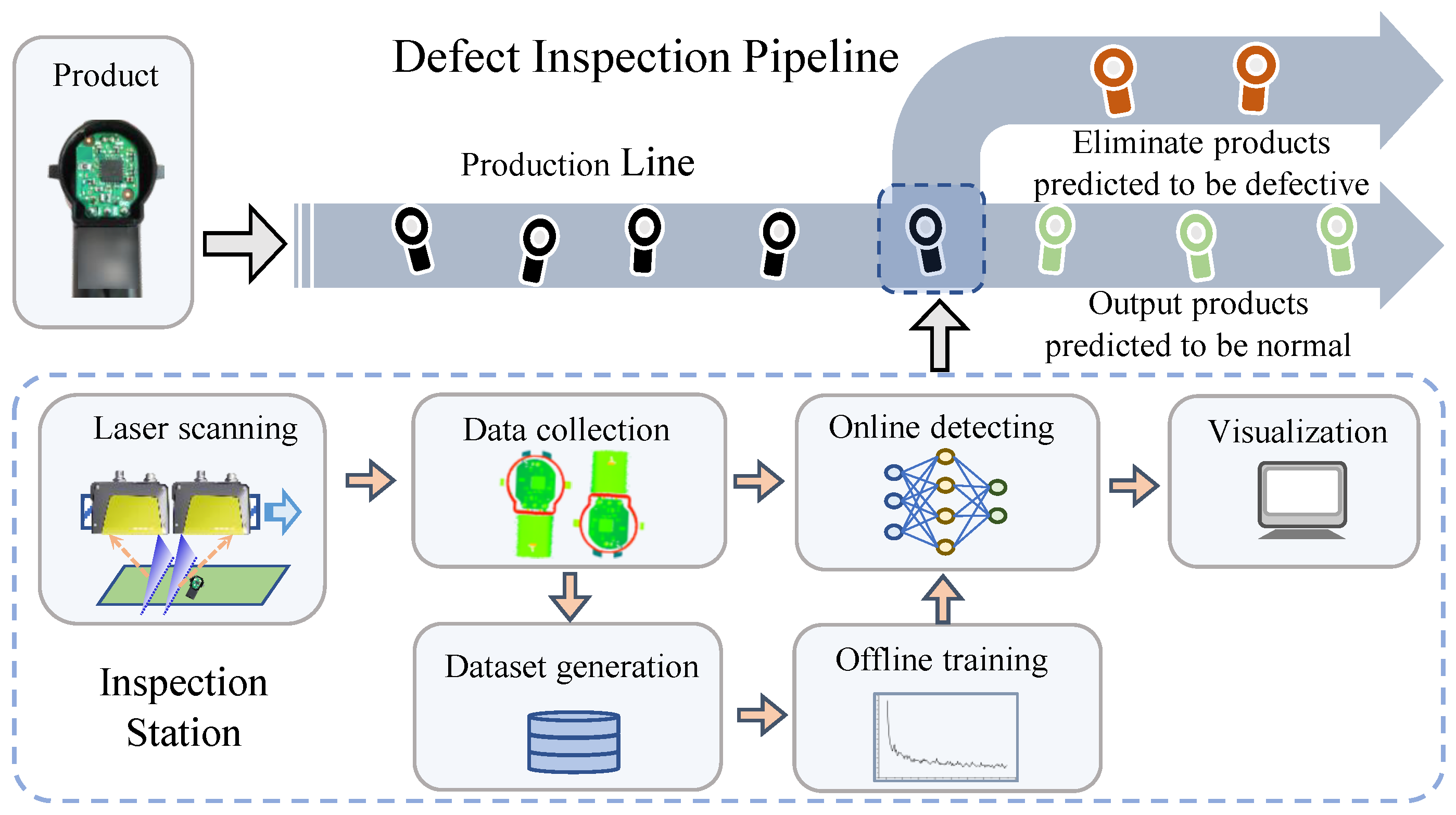
Figure 1. The defect inspection pipeline of the proposed system. In an automotive ultrasonic radar assembly line, the products are inspected online one by one by an model trained offline at the inspection station. The inspection model segments or crops the fixed regions, then makes judgments with a classifier, and the defective products are diverted according to the judgments.
Processes 13 03300 g001
Figure 2. A schematic diagram of PointNet++.
Processes 13 03300 g002
Figure 3. Inspection framework, including recursive segmentation and production classification. The recursive segmentation stage is achieved through N r e c iterative applications of the proposed FSM to the scanned 3D product point cloud, progressively isolating the fixed detection area. Subsequently, a uniquely designed semi-nested point-cloud autoencoder model determines the presence of defects within this segmented region.
Processes 13 03300 g003
Figure 4. Recursive segmentation diagram. By recursively applying N r e c iterations of the proposed FSM, the point cloud of the focal-region point cloud is gradually segmented from the scanned 3D product point-cloud data. The purpose of FSM is to predict the probability of the next sampling after probability sampling so as to continuously focus on a fixed area through recursion.
Processes 13 03300 g004
Figure 5. PointNet++-based focal segmentation module (FSM).
Processes 13 03300 g005
Figure 6. A diagram of rotation-invariant local feature extraction based on LRF.
Processes 13 03300 g006
Figure 7. Semi-Nested Point Cloud Autoencoder (SN-PAE). SN-PAE includes Rotation-Invariant Point Cloud Autoencoder and Latent Autoencoding Module (LAM).
Processes 13 03300 g007
Figure 8. Schematic diagram of the 3D laser scanning system. (a) Schematic diagram of the back-to-back 3D laser scanning mechanism. (b) The scanned point-cloud samples of the left and right views.
Processes 13 03300 g008
Figure 9. Schematic diagram of DHU-RADER1000-ICP and ModelNet40-Toy-AC examples with instance ground truth. (a) Single-view product sample of DHU-RADER1000-ICP. (b) Airplane sample of ModelNet40-Toy-AC. (c) Chair sample of ModelNet40-Toy-AC.
Processes 13 03300 g009
Figure 10. Some samples in DHU-PAD1000-ICP. (a) the original unaligned solder-joint point-cloud samples; (b) the aligned point-cloud samples after ICP.
Processes 13 03300 g010
Figure 11. Visualization of data segmentation results in the segmentation stage.
Processes 13 03300 g011
Figure 12. Experimental results for quantized rotation robustness test. (a) Quantized test of the baseline PonitNet++ on ModelNet40-Toy-AC. (b) Quantized test of the proposed SN-PAE on DHU-PAD1000-ICP.
Processes 13 03300 g012
Table 1. Dataset Partition for Segmentation.
DatasetSample#Train#Test#Total
DHU-RADER1000-ICPNormal9192561175
Defective0256256
ModelNet40-Toy-ACAirplane401252
Chair20626
Table 2. Dataset partition for classification.
DatasetDHU-RADER1000-ICPDHU-PAD1000-ICP
Partition#Train#Test#Total#Train#Test#Total
Normal9192561175521131652
Defective02562560116116
#Total9195121431521237768
Table 3. Experimental results for segmentation stage.
MethodMetricDHU-RADER1000-ICPModelNet40-Toy-AC
Train/%Test/%Train/%Test/%
PointNet++ (LRF)IoU59.267.477.775.7
RandLANet [41]IoU63.269.781.687.4
RIConv++ [10]IoU61.568.179.387.1
Recursive segmentationIoU (k = 1)7382.775.485.7
IoU (k = 2)67.468.1--
Table 4. Comparison of the costs under different settings.
Method#PointsMemory
Cost/MB
Time
Cost/ms
FLOPsParams
PointNet++ (LRF) 1   k 127316.218.5 M0.564 M
PointNet++ (LRF) 10   k 136636.5278.2 M0.564 M
PointNet++ (LRF) 100   k 2946184.83949.8 M0.564 M
PointNet++ (LRF) 300   k 47882839.58112.1 M0.564 M
RandLANet 100   k 5598421.315,456.8 M1.3 M
RandLANet 300   k 14,6721249.146,373.6 M1.3 M
RIConv++ 100   k 3017218.34125.8 M0.436 M
RIConv++ 300   k 49233074.28239.6 M0.436 M
Ours ( N R e c = 1 ) 1   k 120510.321.3 M0.546 M
Ours ( N R e c = 2 ) 10   k 126518.0129.1 M0.614 M
Ours ( N R e c = 3 ) 300   k 136970.4265.3 M0.698 M
Table 5. Comparison results of classification experiments on the DHU-RADER1000-ICP and DHU-PAD1000-ICP datasets.
Model Aligned / Aligned Aligned / Unaligned Augmented / Unaligned
d def min Recall SD d def min Recall SD d def min Recall SD
DHU-PAD1000-ICP
OCCNN [20]06.1-05.3-08.4-
FoldingNet [37]12.879.4-35.422.9-27.330.5-
TargetNet [39]13.780.9-29.532.8-28.137.4-
SN-PAE9.768.6-8.764.9-8.967.9-
DHU-RADER1000-ICP
FoldingNet [37]14.675.30.6228.317.614.724.135.85.3
TargetNet [39]15.278.40.7431.423.715.223.739.24.8
SN-PAE6.9773.80.497.1273.80.516.9373.90.43
Table 6. Results of ablation experiments with SN-PAE on the dataset DHU-RADER1000-ICP DHU-PAD1000-ICP datasets.
SN-PAE Aligned / Aligned Aligned / Unaligned Augmented / Unaligned
LRFLAM d def min Recall SD d def min Recall SD d def min Recall SD
DHU-PAD1000-ICP
13.581.7-38.418.3-33.624.4-
12.678.4-12.878.2-12.678.4-
9.768.6-8.764.9-8.967.9-
DHU-RADER1000-ICP
14.276.90.6726.116.413.720.742.64.6
13.576.10.5213.676.30.5313.576.10.52
6.9773.80.497.1273.80.516.9373.90.43
Disclaimer/Publisher’s Note: The statements, opinions and data contained in all publications are solely those of the individual author(s) and contributor(s) and not of MDPI and/or the editor(s). MDPI and/or the editor(s) disclaim responsibility for any injury to people or property resulting from any ideas, methods, instructions or products referred to in the content.