Article

Interpretable Machine Learning for Shale Gas Productivity Prediction: Western Chongqing Block Case Study

1
Chongqing Shale Gas Exploration and Development Co., Ltd., Chongqing 401123, China
2
College of Energy (College of Modern Shale Gas Industry), Chengdu University of Technology, Chengdu 610059, China
*
Authors to whom correspondence should be addressed.
Processes 2025, 13(10), 3279; https://doi.org/10.3390/pr13103279
Submission received: 17 August 2025 / Revised: 1 October 2025 / Accepted: 9 October 2025 / Published: 14 October 2025
(This article belongs to the Special Issue Numerical Simulation and Application of Flow in Porous Media)

Abstract

The strong heterogeneity in and complex engineering conditions of deep shale gas reservoirs make productivity prediction challenging, especially in nascent blocks where data is scarce. This scarcity constitutes a critical research gap for the application of data-driven methods. To bridge this gap, we develop an interpretable framework by combining grey relational analysis (GRA) with three machine learning algorithms: Random Forest (RF), Support Vector Machine (SVR), and eXtreme Gradient Boosting (XGBoost). Utilizing small-sample data from 87 shale gas wells in the study area, eight key controlling factors were identified, namely, total fracturing fluid volume, proppant intensity, average tubing head pressure, pipeline transfer pressure, casing head pressure, ceramic proppant fraction, fluid placement intensity, and flowback recovery ratio. These factors were used to train, optimize, and validate a productivity prediction model tailored for deep shale gas horizontal wells. The results demonstrate that XGBoost delivers the highest predictive accuracy and generalization capability, achieving an R2 of 0.907 for productivity prediction—surpassing RF and SVR by 12.11% and 131.38%, respectively. Integrating SHapley Additive exPlanations (SHAP) interpretability analysis further enabled immediate post-fracturing productivity assessment and engineering parameter optimization. This research provides a reliable, data-driven strategy for predicting productivity and optimizing operations within the studied block, offering a valuable template for development in geologically similar areas.

1. Introduction

Shale gas, a vital clean and low-carbon fossil energy resource, plays a key supporting role in realizing “dual-carbon” strategic objectives [1]. Deep shale gas reservoirs possess far greater geological and fracturing operational complexity than conventional mid-shallow reservoirs, in which characteristic nanoscale pore structures exhibit fluid flow with significant non-Darcy behavior. Additionally, the coupled flow mechanisms of multiphase fluids are complex under high-temperature, high-pressure geological conditions, resulting in a rapid exponential production decline. Field data demonstrate that 180–240 days of systematic production testing are required to acquire stabilized gas rate data from deep shale gas wells, while exploration well density is merely 20% of that in shallow plays. This conflict between “unsteady-state flow” production characteristics, scarce sample data, and prolonged testing periods introduces substantial uncertainty into productivity prediction [2,3]. For instance, in the Western Chongqing Block, deep shale reservoirs exhibit intense structural deformation, significant spatial heterogeneity in gas content, and complex fracture networks induced by large-scale volumetric fracturing, collectively complicating quantitative productivity evaluation. Consequently, developing accurate productivity prediction models carries significant engineering value for designing scientific development strategies and improving economic returns [4,5,6].
However, traditional methods, such as numerical simulation based on physical principles, often struggle with the aforementioned complexities and, crucially, require extensive and precise geological and fluid data, which are typically scarce and costly to obtain in nascent blocks like Western Chongqing [7,8]. This limitation hinders their practical application during early development phases. Facing this “data scarcity” challenge, data-driven machine learning (ML) methods offer a compelling alternative. ML models can learn complex nonlinear relationships directly from available operational data, bypassing the need for explicit physical modeling and detailed geological parameters. In this study, we adopted this approach, utilizing a set of key and readily available operational parameters—such as fracturing fluid volume, proppant intensity, and wellhead pressures—that are routinely monitored and have a direct, interpretable impact on productivity. To address the critical need for early-stage decision support under data constraints, a practical and interpretable model was built by leveraging these parameters from 87 wells [9,10,11].
Current mainstream approaches for shale gas productivity prediction primarily include analytical flow models, numerical simulations, and empirical formulas [12]. Analytical methods based on point-source functions and conformal mapping theory offer computational efficiency but suffer accuracy limitations because they oversimplify the complex flow mechanisms of shale gas. Numerical simulations that couple multi-physical processes, like adsorption–desorption and slip flow, excel in mechanistic representation; however, they are hindered by high uncertainty in fracture network geometry modeling, intensive computational requirements, and strong dependence on manual calibration. Empirical formulas (e.g., production decline analysis) exhibit poor generalization and heavy reliance on expert judgment owing to geological heterogeneity and spatial parameter variability [13,14]. These limitations are amplified in deep shale gas development: high closure stress invalidates the core assumptions of analytical models; complex fracture topologies increase numerical solution uncertainty; and inter-block geological–engineering disparities magnify extrapolation errors in empirical methods [15].
Machine learning methods address these limitations through data-driven approaches that directly extract complex mappings between geological–engineering parameters and productivity while eliminating reliance on physical mechanism assumptions. In recent decades, researchers have developed diverse ML models for gas well performance prediction, establishing relatively mature methodologies. Rumelhart et al. pioneered the multilayer neural network and backpropagation (BP) algorithm, laying the groundwork for ANN development [16]. MENG et al. (2015) demonstrated SVM’s superior accuracy over BP neural networks for small datasets using various kernel functions [17]. Hui et al. (2021) integrated geological/operational factors in shale gas production prediction and compared linear regression, neural networks, gradient boosting decision trees, and extra trees—identifying random forest as the optimal productivity prediction model [18]. Song et al. (2023) developed productivity prediction models using five ML algorithms, with comparative evaluation showing LightGBM’s superior stability and generalization [19]. Hamid et al. (2024) fine-tuned ML hyperparameters to establish a two-layer ANN production forecasting model, combining it with the MDE algorithm for well productivity optimization [20]. GUAN et al. (2025) enhanced productivity prediction accuracy for southern Sichuan shale gas infill wells using grey wolf algorithm-optimized LSTM with staged modeling [21]. Beyond prediction, the application of ML extends to production optimization, where understanding the impact of controllable parameters is key. In this domain, Support Vector Machines (SVMs) have been valued for their ability to model complex, nonlinear relationships between engineering parameters and outcomes, even with limited data, providing a robust basis for identifying optimal operational windows. For instance, Wang and Chen (2019c) demonstrated the comparative power of ML models by screening 6 key features from 11 initial productivity factors and establishing prediction models, finding that the Random Forest model outperformed Adaptive Boosting, SVM, and neural network methods [22]. Similarly, the eXtreme Gradient Boosting (XGBoost) algorithm has demonstrated exceptional performance in feature selection and ranking parameter importance, making it a powerful tool for pinpointing the most influential productivity enhancement factors in shale gas development. Notably, Zhou et al. (2024) developed an ASGA-XGBoost model that significantly improved the accuracy of shale gas production prediction by optimizing hyperparameters, providing strategic support for the economic and efficient development of shale gas fields [23]. The combination of these powerful predictive models with interpretability frameworks, like SHAP, is particularly suited for translating model insights into actionable optimization strategies.
For ML interpretability, Guevara et al. (2018) integrated domain knowledge with expert experience to build interpretable ML for engineering decisions [24]. WANG et al. (2019) created a data mining framework to evaluate Montney Formation well performance, quantitatively linking stimulation parameters to first-year oil production [22]. Liu et al. (2021) proposed a “gray-box” model fusing physical priors with ML for unconventional reservoir forecasting, enabling partial interpretability [25]. Castro et al. (2023) leveraged Random Forests and production data to derive causal relationships through feature importance, constructing corresponding causal networks [26].
Although machine learning has achieved certain success in oil and gas productivity prediction, it faces three major engineering application bottlenecks in deep shale gas development: First, the sample acquisition challenge is prominent, with typically fewer than 100 available samples for deep shale gas wells, significantly below the minimum requirement of 200 wells for algorithms such as Random Forest, LightGBM, and ANN [18,19,20]. This leads to increased overfitting risks under small-sample conditions, while high-quality data acquisition and processing costs remain prohibitively high. Second, model interpretability is insufficient; existing “black-box” prediction methods struggle to reveal threshold mechanism relationships between fracturing parameters and productivity. Even with advanced interpretation methods, engineering application disconnections persist [22,24,26]. Finally, for early development wells lacking comprehensive geological data, lengthy data preparation cycles and high costs severely constrain the timeliness of engineering decisions. These critical bottlenecks must be resolved immediately to achieve efficient deep shale gas development. The combination of these powerful predictive models, like XGBoost and SVM, with interpretability frameworks is particularly suited for translating model insights into actionable optimization strategies.
Guided by engineering operability principles, this research systematically identified eight key productivity-controlling factors: total fracturing fluid volume, proppant intensity, average tubing head pressure, pipeline transfer pressure, casing head pressure, ceramic proppant fraction, fluid placement intensity, and flowback recovery ratio. Gray relational analysis quantitatively confirmed strong correlations between these parameters and productivity. With selected features as inputs and stabilized gas rate as the prediction target, a comparative framework was established using three intelligent models: Support Vector Machine (SVM), Random Forest (RF), and XGBoost. The XGBoost model—enhanced by second-order Taylor expansion for loss function optimization and regularization mechanisms—achieved superior performance on actual production data from 87 deep shale gas wells, attaining a test set R2 of 0.907. This model outperformed the RF and SVM models by 12.11% and 131.38%, respectively. SHapley Additive exPlanations (SHAP) interpretability analysis further quantified the parameter contribution rankings to productivity and enabled sensitivity-based tiered control strategies. This methodology transcends traditional approaches’ reliance on empirical parameters and sample size constraints while substantially accelerating prediction timelines for real-time field decisions. Critically, field implementation in Western Chongqing’s deep shale gas reservoirs confined post-fracturing productivity prediction errors within 5%, demonstrating robust technical support for efficient development in geologically complex settings [27,28,29,30].

2. Data and Methods

2.1. Data Sources

The dataset utilized in this study comprised production data from 87 individual horizontal shale gas wells in the Western Chongqing Block. The data were sourced from the “Chongqing Shale Gas Daily Report”—a production field data compilation table—and included daily production metrics up to May 2025. To ensure data stability and representativeness for productivity prediction, the final stabilized daily gas rate was selected as the target variable (productivity label) for each well. This approach aimed to provide real-time insights and data-driven strategies for optimizing development indicators, forecasting production potential, and guiding subsequent development decisions in this actively developing block.
In this study, we utilized data from 87 gas wells across Blocks Z201, Z203, and Z206 in the Western Chongqing Gas Field. Guided by engineering operability and data integrity requirements for direct productivity control, we selected fracturing parameters: total fracturing fluid volume, proppant intensity, ceramic proppant fraction, and fluid placement intensity. Concurrently, based on monitoring significance and real-time constraints, production parameters—pipeline transfer pressure, casing head pressure, average tubing head pressure, and flowback recovery ratio—were identified. This established a focused parameter system comprising eight key engineering variables (Table 1), spanning fracturing design and production dynamics. All feature data were extracted from drilling reports, fracturing design documents, and early production records of the 87 wells.
The selection of these operational and production parameters (as listed in Table 1) was based on both industry standards and practical data availability. Key parameters, such as proppant intensity, fluid volume, and wellhead pressures, are explicitly recommended and defined in the Chinese national and industry standards for shale gas production prediction (GB/T 41612-2022 and NB/T 14024-2017) [31,32], reflecting their critical role in evaluating fracture effectiveness and forecasting well productivity. Furthermore, this selection was pragmatically guided by data accessibility and integrity from ongoing development projects. These parameters are routinely and reliably recorded in field production reports (e.g., the “Chongqing Shale Gas Daily Report”), making them not only scientifically valid but also highly practical. This approach is particularly advantageous for developing blocks, like Western Chongqing, or for mature fields with incomplete historical geological data, as it leverages commonly available high-quality operational data to build robust models. It ensures the model’s applicability and provides a replicable framework for production forecasting and optimization in analogous shale gas assets [33,34].
Parameter system development followed the “data-driven decision making” principle:
  • Initial identification of full parameter sets (including geological parameters) through a comprehensive well history review.
  • Selection of high-integrity parameters via data quality evaluation. Prioritizing parameters with complete engineering monitoring records maintained dataset integrity and prevented interpolation bias.
As Table 2 demonstrates, the chosen parameters showed substantially lower missing data rates than the geological parameters and satisfied model input frequency criteria. This approach ensured model robustness while conforming to practical engineering data constraints.
Furthermore, adhering to the “engineering-dominated” productivity theory for shale gas (King, 2010) [35], engineering parameters account for 78–92% of productivity variability when reservoir quality is comparable. In this study, we constructed a parameter system that spans the full spectrum of fracturing design and production management, embodying the contemporary paradigm of “converting geological sweet spots to engineering sweet spots”.
In the preprocessing analysis of daily gas production data, the raw data exhibited a significantly right-skewed distribution, with the mean (4.11 × 10⁴ m3/d) substantially higher than the median (2.97 × 10⁴ m3/d), indicating a strong influence of high-end outliers on the data distribution. By applying statistically principled outlier treatment methods (such as the IQR method or Winsorization), the distribution morphology of the processed data was notably improved. The mean of the processed data decreased to 3.78 × 10⁴ m3/d, while the median remained stable (2.97 × 10⁴ m3/d) as shown in Figure 1. Concurrently, the boxplot revealed a significant reduction in the number of outliers and a decrease in data dispersion. This preprocessing strategy effectively mitigated the distorting effect of extreme values on the data distribution, resulting in a more concentrated and symmetrical data profile. This lays a solid data foundation for subsequent machine learning modeling, contributing to enhanced stability in model training and improved prediction accuracy. Algorithms particularly sensitive to outliers, such as regression techniques and gradient-based optimization models, are expected to benefit substantially from this treatment.
Additionally, since the Yuxi gas field data used in this study include feature variables with different dimensions and vastly different ranges, failure to process them would cause the prediction model to fail to converge. Therefore, data normalization was required. Normalization, a common method to eliminate dimensional effects, linearly transforms data, mapping the results to the [0, 1] range. This process reduces scale disparities by rendering the data dimensionless. The transformation function is as follows:
X = X min X max X min X
where min X is the minimum value of the data, max X is the maximum value of the data, and X is the normalized data.
For model performance evaluation, we employed four core metrics for a comprehensive assessment: coefficient of determination (R2), mean squared error (MSE), root mean squared error (RMSE), and mean absolute error (MAE). The coefficient of determination (R2), a key indicator of the goodness-of-fit for regression models, is calculated as follows:
R 2 = 1 i = 1 n y i y ^ i 2 i = 1 n y i y i ¯ 2
where y i is the target value, y ^ i is the predicted value of the model, and y i ¯ is the mean value of all target values. The range of R2 is [0, 1]. Its statistical significance lies in quantifying the proportion of the dependent variable’s variation explained by the regression equation: when R2 approaches 1, the regression sums of squares accounts for a high proportion of the total sum of squares, signifying strong model explanatory ability; conversely, when it approaches 0, the model fails to effectively capture the underlying data variability.
The mean square error MSE is defined as
1 n i = 1 n y i y ^ i 2
This metric takes values in the interval [0, +∞), with smaller values indicating higher model prediction accuracy. As a widely adopted loss function in machine learning, MSE penalizes large errors more heavily through the squaring operation, making it more sensitive to outliers. Additionally, it possesses good continuous differentiability, supporting gradient-based optimization algorithms.
Root mean squared error (RMSE) is defined by the equation:
1 n i = 1 n ( y i y ^ i ) 2
This metric takes values in [0, +∞), where lower values correspond to higher prediction precision. Derived from MSE, RMSE applies squaring followed by square-rooting—retaining strong penalty sensitivity for large errors while reconciling error units with the original data. Its continuous differentiability (except at zero) facilitates gradient-based optimization.
Mean absolute error (MAE) is defined by the equation
1 n i = 1 n | y i y ^ i |
Taking values in [0, +∞), a lower MAE indicates superior prediction accuracy. This robust loss function mitigates squared amplification of large errors with absolute difference computation, reducing outlier interference. MAE maintains physical unit consistency with the original data, enabling intuitive quantification of average prediction deviation.
These four metrics form a synergistic evaluation framework: R2 quantifies model explanatory capacity, MSE gauges absolute error intensity, RMSE standardizes error dimensionality, and MAE diagnoses prediction robustness—jointly guaranteeing comprehensive and reliable regression model assessment.

2.2. Grey Correlation Analysis

Grey relational analysis (GRA) is a quantitative comparison method for multi-factor systems [36]. Its theoretical core lies in characterizing the strength, magnitude, and order of relationships between factors through the similarity degree of their evolutionary curve trends [37]. The closer the geometric shapes of two-factor sequences during their evolution, the higher their gray relational grade, reflecting stronger intrinsic synergy; conversely, the lower the relational grade, the weaker the system coupling [38].
In this study, daily gas production was used as the reference sequence (parent sequence), while engineering production parameters—including total fracturing fluid volume, proppant intensity, tubing head pressure, pipeline transfer pressure, casing head pressure, ceramic proppant fraction, fluid placement intensity, and flowback recovery ratio—were used as the comparative sequences (sub-sequences) [39,40]. The specific calculation process is as follows:
Daily gas production is selected as the reference sequence, and the engineering and production parameters are the comparative sequences, denoted as
X 0 = X 0 1 , X 0 2 , X 0 3 , , X 0 n X i = X i 1 , X i 2 , X i 3 , , X i n X m = X m 1 , X m 2 , X m 3 , , X m n
where X 0 is the reference sequence; X i is the comparison sequence; j i = 0, 1, 2…, m ; and k = 1, 2…, n .
Given that each variable has different units and different scales, each data point must be transformed to create a variable under a certain normative scale. To ensure that each data point has equal polarity and weight, it is necessary to normalize the data points and remove their dimensions. The initial value method is used to remove the dimensions of the data; the optimal sequence is selected first, which is denoted as { x 0 1 , x 1 1 , x n 1 } . The formula is as follows:
Y j k = X j k X j 1
where Y j k is the dimensionless sequence.
Next, the difference sequence is used to calculate the formula as follows:
Δ 0 i k = Y 0 k Y i k
where Δ 0 i k is the absolute difference.
The maximum and minimum difference in the two levels is calculated as
Δ max = max i max k Y 0 k Y i k
Δ min = max i max k Y 0 k Y i k
where Δ max is the two-level maximum difference, and Δ min is the two-level minimum difference.
The correlation coefficient is calculated as follows:
ξ 0 ι k = Δ min + ρ Δ max Δ 0 i k + ρ Δ max
where ρ is the resolution coefficient. Its role is to improve the significance of the difference between the correlation coefficients, ρ ∈ (0, 1), and it usually takes the value of 0.5. The smaller the value of ρ, the more it can improve the difference between the correlation coefficients.
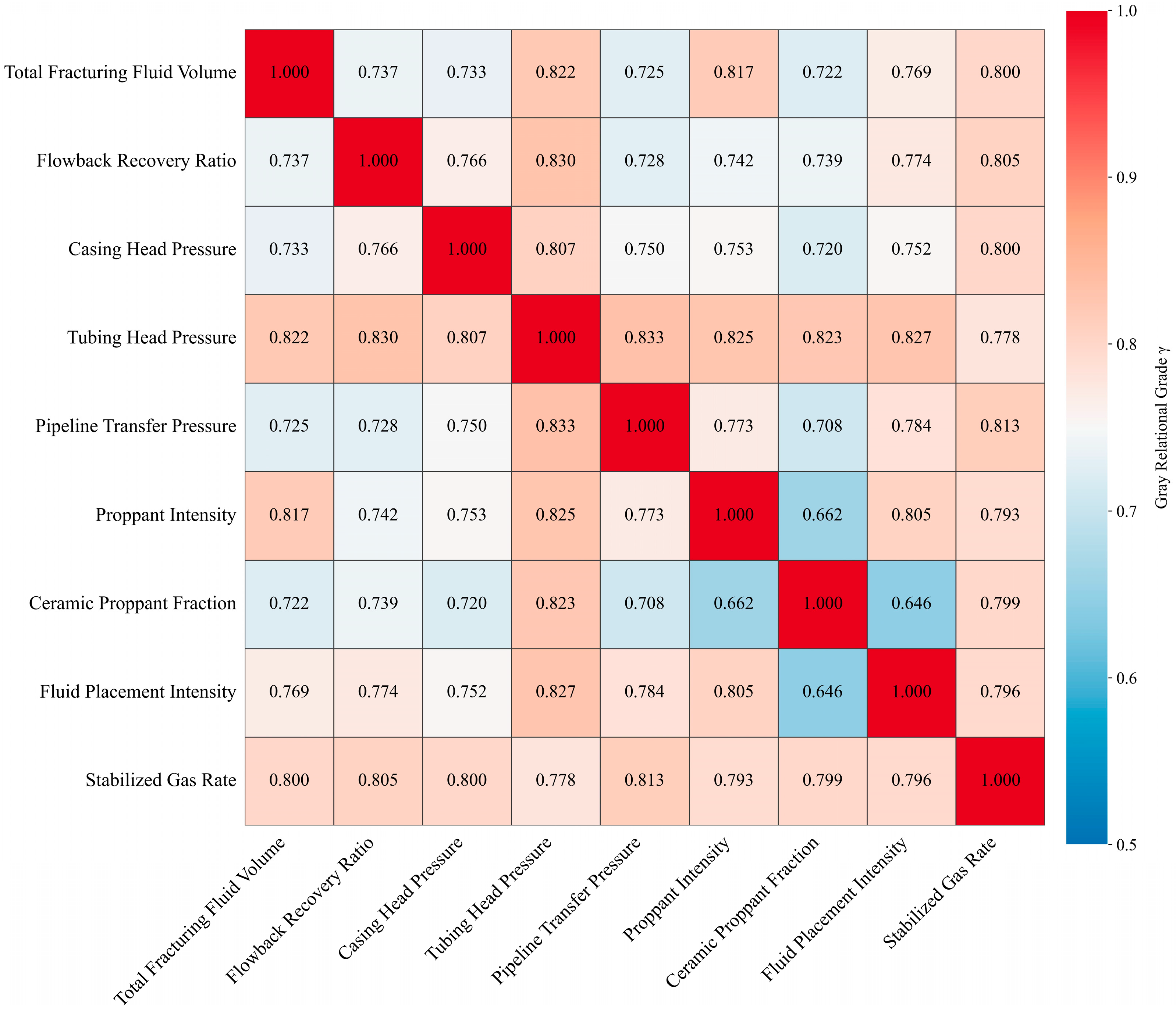
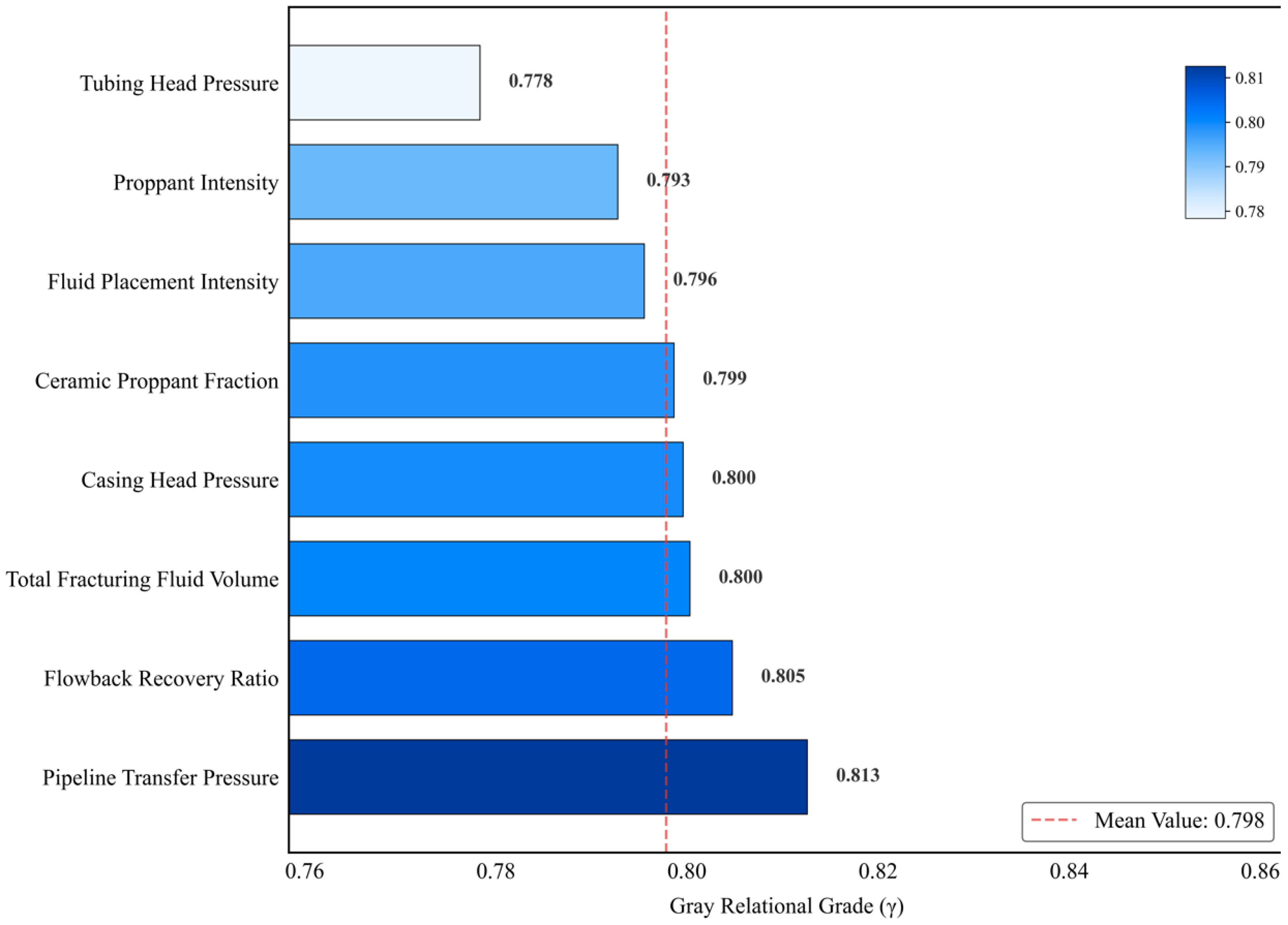
According to the above steps, a diagram illustrating the influence of the main control factors on gas well productivity in the Yuxi Block is obtained (Figure 2). The gray relational grades of all factors are above 0.778, with an average value of 0.798, demonstrating a strong association between the selected factors and daily gas productivity (Figure 3). This verifies the scientific validity of the previous feature screening. Pipeline transfer pressure exhibits the highest relational grade, indicating its strongest association with the daily productivity of shale gas.

2.3. Machine Learning Models

Given the small dataset (87 wells), high nonlinearity, and multidimensional heterogeneity from combined production/operational parameters in gas well productivity forecasting, we implemented three algorithms with robust nonlinear modeling capabilities: Support Vector Regression (SVR), Random Forest Regression (RF), and eXtreme Gradient Boosting (XGBoost) for model development and selection. Hyperparameters were determined through an iterative grid search aimed at improving cross-validation performance on the training set. The final values, presented in the tables in Section 2.3, represent the optimal configuration for each model.

2.3.1. Support Vector Regression

Support Vector Regression (SVR) utilizes the Radial Basis Function (RBF) kernel to map features into a high-dimensional space and find an optimal hyperplane that keeps the samples within the ϵ-insensitive band [41]. SVR aims to find this optimal regression hyperplane by minimizing an ϵ-insensitive loss function, meaning most sample points lie between the two boundary lines (Figure 4). In productivity prediction, the kernel function flexibly fits the nonlinear relationship between input features and productivity, while the ϵ-insensitive band controls the model’s generalization ability.
The Support Vector Regression (SVR) algorithm processes non-linearly separable data by first mapping the original samples into a higher-dimensional feature space via a kernel function. This transformation converts the originally non-linearly separable data in low-dimensional space into a linearly separable problem in high-dimensional space. Within this new space, the algorithm identifies an optimal hyperplane that maximizes the margin between two classes of samples. Specifically, it locates the hyperplane that maximizes the minimum distance from the nearest sample points (support vectors) to the hyperplane. Based on this constructed hyperplane, regression predictions are made according to the distance between new samples and the hyperplane. The predicted values correspond to the target variable magnitudes of new samples.
The penalty factor C is defined by Equation (12):
C = 1 2 w 2 + λ n = 1 N C n C n = max y Δ y ^ n , y + w ϕ x n , y w ϕ x n , y ^ n
The Gaussian kernel function is expressed as
K x , z = exp x z 2 2 σ 2
For the Support Vector Machine model, the radial basis function (RBF) kernel was selected to resolve the nonlinear relationship between fracturing parameters and productivity via high-dimensional mapping. To balance margin width against training errors while controlling local sample influence and preventing overfitting, the penalty factor C and kernel coefficient gamma were set to 1.0 (Table 3).

2.3.2. Random Forest Regression

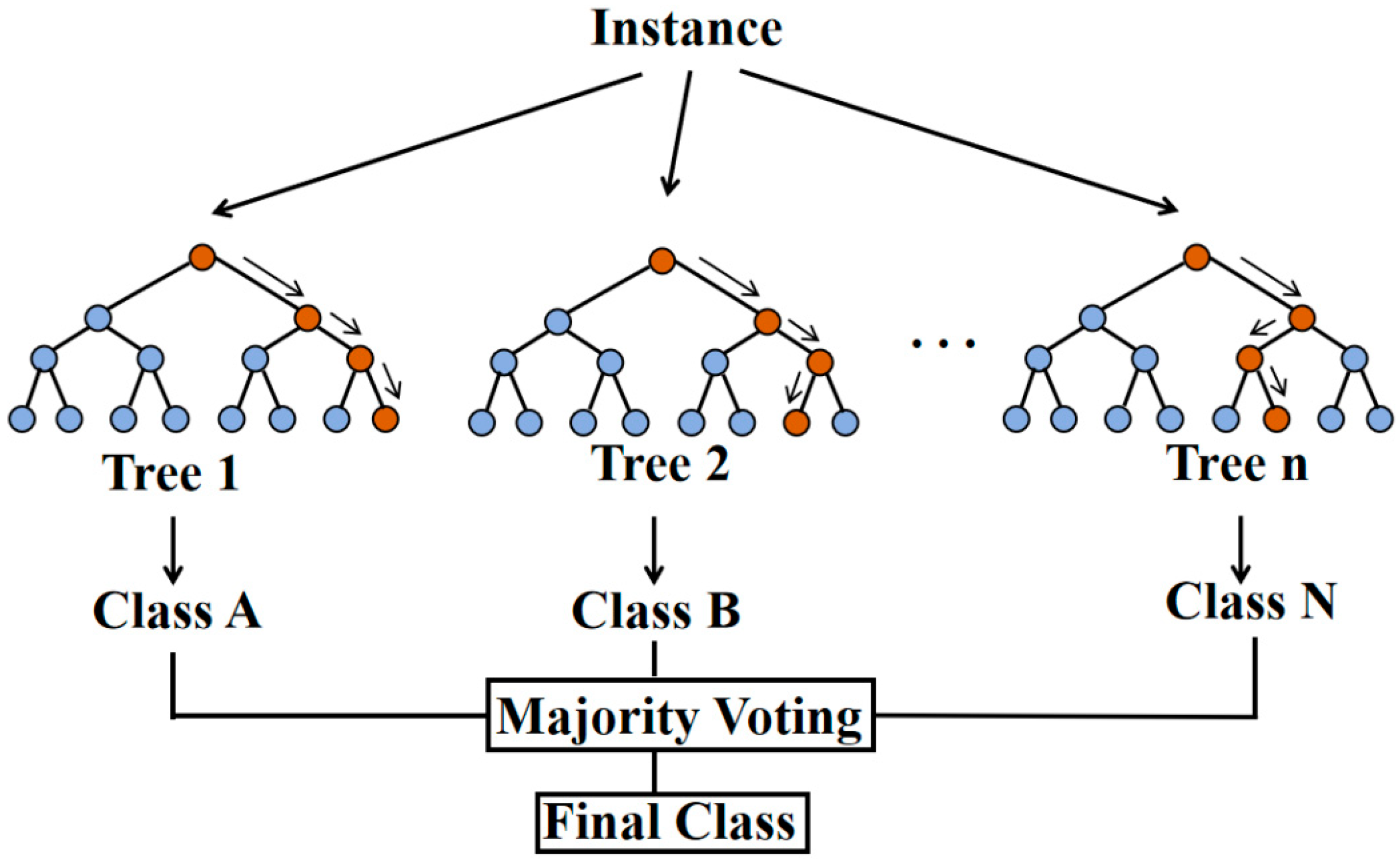
Random Forest Regression (RF), based on Bagging integration and Gini index splitting (Equation (14)), constructs multiple independent decision trees operating in parallel [42]. This ensemble framework enables parallel prediction (Figure 5), facilitating automatic assessment of feature importance (e.g., total fracturing fluid volume, flowback recovery ratio) with stability verified via out-of-bag error.
min j s min c 1 x i R 1 j , s y i c 1 2 + min c 2 x i R 2 j , s y i c 2 2
where xi denotes the input at each node, yi is the corresponding output, and cm represents the optimal output weight. This weight is determined by computing the mean of the output values yi corresponding to all inputs xi within each node:
c ^ m = a v e r a g e y i x i R m
when predicting shale gas well productivity indicators, single decision trees may yield significant errors due to overfitting risks. Therefore, the Random Forest model ensembles multiple decision trees, with final predictions generated by averaging individual tree outputs to enhance accuracy.
As a small-sample prediction model, parameter optimization requires strict control of tree complexity to prevent overfitting. The key parameters optimized in this study include the number of trees (n_estimators = 300) and maximum depth (max_depth = 3), which constrain model complexity (Table 4).

2.3.3. eXtreme Gradient Boosting

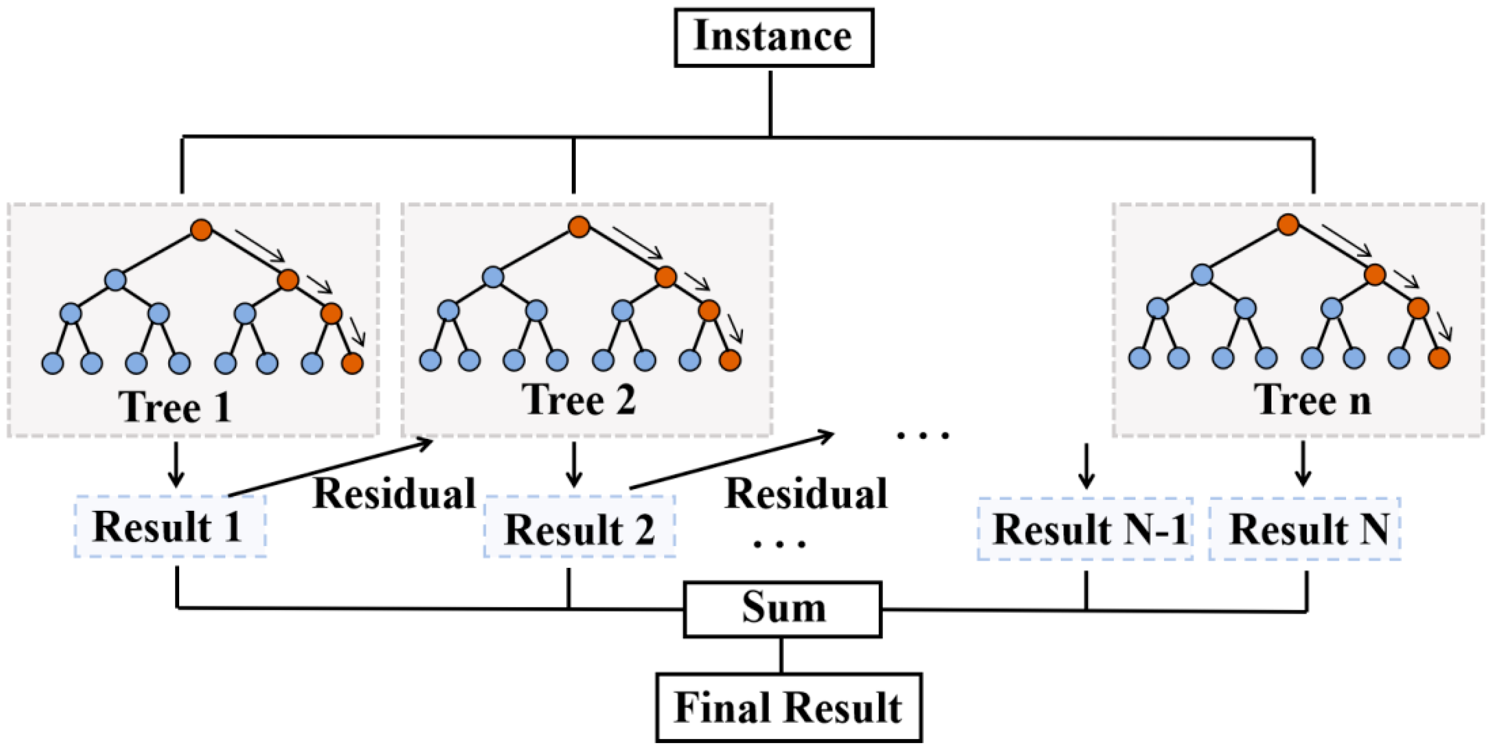
eXtreme Gradient Boosting (XGBoost) optimizes the loss function via second-order Taylor expansion and iteratively adds weak learners to enhance prediction accuracy. As a Boosting-based algorithm [43], it sequentially transfers previous computation results to subsequent iterations, with its specific workflow illustrated in Figure 6. For shale gas well productivity prediction, regularization terms suppress small-sample overfitting while automatically handling missing features and outliers.
According to the forward stagewise additive modeling framework, assuming the base model at the t-th iteration is f t x i , the model update is defined as follows:
y ^ i t = k = 1 t y ^ i t 1 + f t x i
The XGBoost loss function consists of an empirical loss term and a regularization term:
L = i = 1 n l y i , y ^ i + i = 1 t Ω f i
where i = 1 n l y i , y ^ i is the empirical loss term, indicating the loss between the predicted value and the true value of the training data, and i = 1 t Ω f t is the regularization term, indicating the sum of the complexity of all t trees, which is also the method that XGBoost uses to control the overfitting of the model.
When defining the regularization term of the decision tree, the model complexity Ω can be determined by the number of leaf nodes T and leaf weights w of a single decision tree, i.e., the complexity of the loss function is determined by the number of all leaf nodes and leaf weights in the decision tree. So, the complexity of the model can be expressed as
Ω f t = γ T + 1 2 λ j = 1 T w j 2
The information gain after splitting is
G a i n = 1 2 G L 2 H L + λ + G R 2 H R + λ G L + G R 2 H L + H R + λ γ
Given the small-sample characteristics and nonlinear nature of shale gas well productivity prediction in the Yuxi Block, our model parameterization prioritized overfitting prevention through tree depth constraints, enhanced regularization, computational efficiency balance, base learner quantity control, and preserved feature importance analysis [44]. The optimized parameters for the XGBoost productivity prediction model are summarized in Table 5.
By building on the fundamental principles of the three algorithms, productivity prediction models were established using productivity data as the objective function. Feature importance was computed and ranked to form the modeling foundation. The workflow (Figure 7) encompasses productivity prediction for target-block shale gas wells and comparative model selection.

2.4. SHAP Interpretability Mechanisms

The SHAP interpretability framework, rooted in cooperative game theory’s Shapley values [45], quantifies feature contributions to machine learning outputs via an axiomatic approach. Its core decomposes model predictions into additive components: a baseline expectation plus individual feature contributions. Shapley values are computed as the mean marginal contribution over all possible feature subsets.
For tree-based models, the TreeSHAP algorithm leverages decision path backtracking to dynamically track feature splitting gains. It aggregates contributions through path probability weighting [46]. This method provides mathematically rigorous explanations of black-box models by quantifying nonlinear feature effects and interactions. With polynomial time complexity enabled by tree path traversal, TreeSHAP offers operational efficiency for engineering decisions.

3. Experimental Results and Discussion

3.1. Model Performance Comparison and Optimization

We selected Support Vector Machine (SVM) among single models, along with XGBoost and Random Forest (RF) from ensemble learning, for productivity prediction. All three models were trained using stabilized gas rate as the label, with eight dominant factors screened as input parameters. Through comparative analysis of model simulation results and evaluation metrics, the optimal predictive model among the three types was identified.
A comprehensive comparison of SVR, RF, and XGBoost performance on identical training and test sets (Table 6) demonstrates XGBoost’s significant advantages in productivity prediction. It achieved the lowest RMSE, MAE, and MSE on the test set—significantly lower than RF and SVR—while attaining the highest R2 (0.907) with minimal deviation from training set performance. This confirms XGBoost’s superior prediction accuracy, minimal errors, strong generalization capability, and low risk of overfitting. In contrast, SVR exhibited severe performance degradation on the test set (R2 = 0.392) despite an adequate training fit. RF maintained robustness (R2 ≈ 0.81 across sets) but remained below 0.85, indicating inferior accuracy compared to XGBoost.
Figure 8 comprises six subplots, presenting productivity prediction regression curve analyses for the three ML models—Support Vector Machine (SVM), Random Forest (RF), and XGBoost—on the training and test sets. Each model includes prediction comparisons for the training set (a1, b1, c1) and the test set (a2, b2, c2). The scatter points represent the observed versus predicted values, with the red diagonal line (y = x) indicating the ideal prediction. Overall, all models exhibit strong alignment with the diagonal line in the training sets (a1, b1, c1), where the points cluster tightly along the black regression line and the diagonal, confirming effective learning from the training data.
XGBoost (c1) demonstrates optimal fitting performance, with the scatter points highly concentrated near the 45° reference line (R2 = 0.924). RF (b1) also performs robustly, showing minimal average deviation (0.08) from the diagonal. In contrast, SVM (a1) displays significantly higher dispersion; its regression curve notably deviates in high-production regions (>15 × 104 m3/d), indicating limited extreme value capture capability.
For test set visualizations, XGBoost (c2) maintains superior generalization, with predictions closely adhering to the diagonal, except for a minor deviation at peak productivity (>15 × 104 m3/d, R2 = 0.907). RF (b2) shows moderate performance (R2 = 0.809), with slight divergence in low-productivity zones (<5 × 10⁴ m3/d). SVM (a2) fails severely (R2 = 0.392), exhibiting random dispersion and pronounced deviations in high-productivity regions (>5 × 10⁴ m3/d).
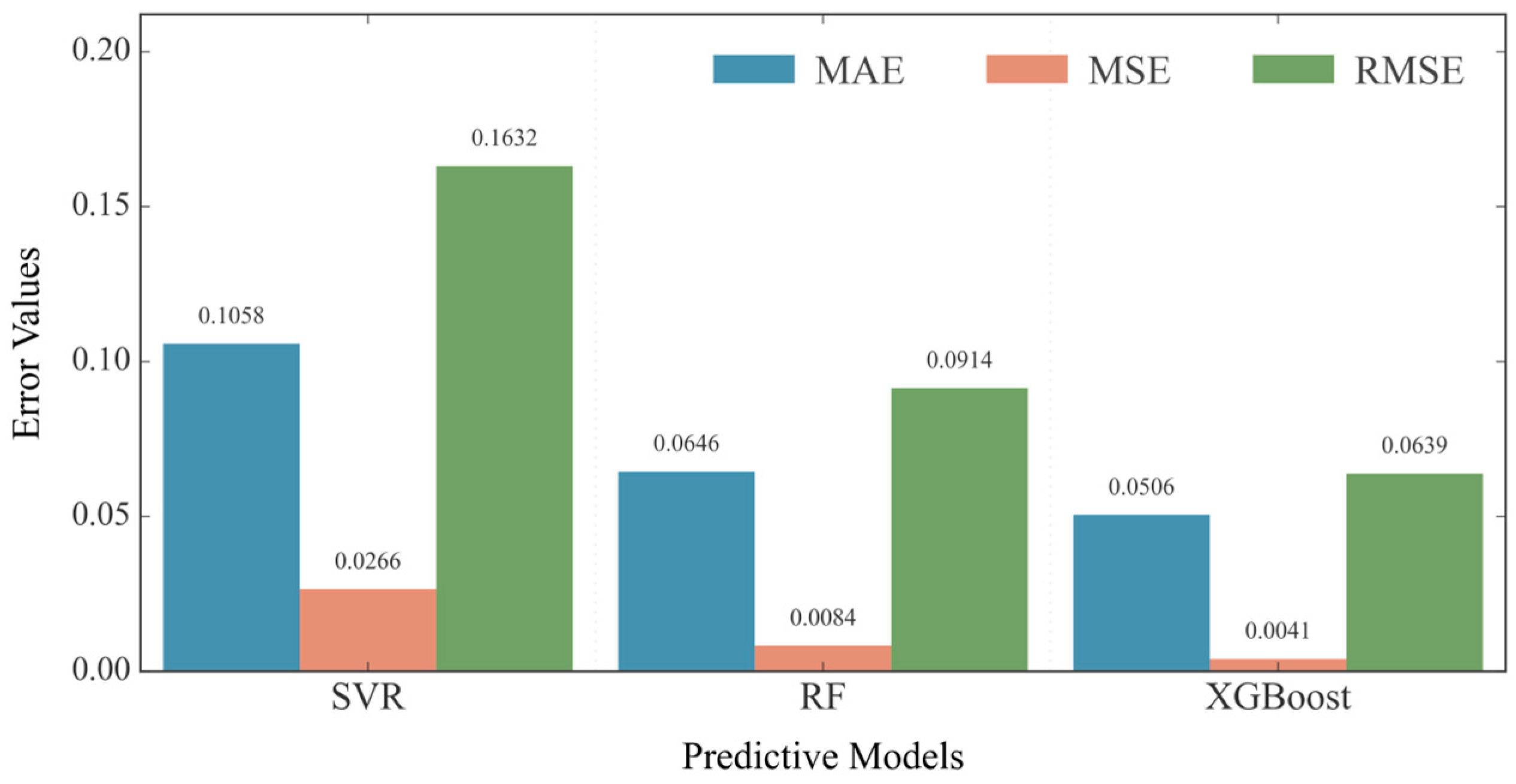
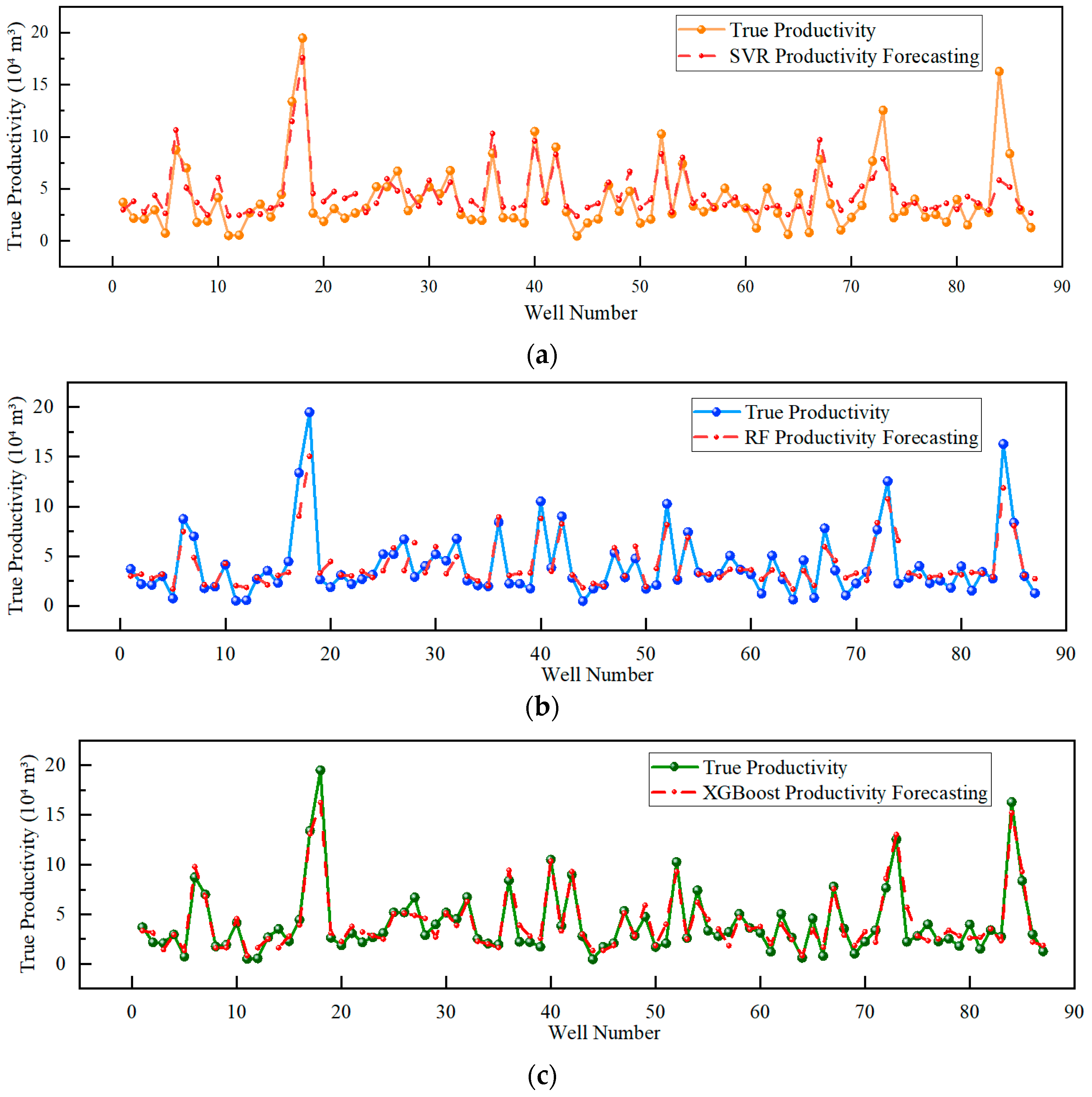
Regarding the test set metrics (Figure 9), Figure 10 displays the SVR (a), RF (b), and XGBoost (c) error profiles. XGBoost (c) exhibits superior error containment—the curve is tightly bound to the zero-deviation line without outliers—achieving minimal test set RMSE (0.06393) and MAE (0.05059), suggesting robust stability. RF (b) shows moderate error control but oscillates in low-yield regions (<50,000 m3/d); its 0.09143 RMSE is 43.1% higher than that of XGBoost, confirming an accuracy deficit. SVR (a) catastrophically fails, with violently divergent errors and systematic positive bias across all ranges: its RMSE reaches 2.55× XGBoost’s value, while the R2 collapse reveals critical overfitting and generalization deficiencies.
Based on our comprehensive analysis, although all three models effectively fit the training data, their generalization performance diverges significantly on the test set. The XGBoost model demonstrates superior prediction accuracy and generalization capability, delivering highly consistent and accurate test set results. Random Forest exhibits good generalization but comparatively lower predictive precision. The Support Vector Machine (SVM) model underperforms, showing systematic underestimation and high prediction dispersion on the test set. These results highlight XGBoost’s advantages for productivity prediction tasks.

3.2. Cross-Validation and Statistical Significance Analysis

While a single train–test split provides an initial performance estimate, its results can be susceptible to the randomness of the data partitioning. To perform a more stable and reliable evaluation, we systematically employed a five-fold cross-validation scheme. Furthermore, the cross-validation results were subjected to a comprehensive statistical significance analysis, including Analysis of Variance (ANOVA), Tukey’s Honest Significant Difference (HSD) post hoc test, and the calculation of 95% confidence intervals. This integrated framework was designed to facilitate a statistically grounded comparison of predictive performance among the XGBoost, Random Forest, and Support Vector Machine (SVM) models.
The results of the five-fold cross-validation are summarized in Table 7. The data indicate that the XGBoost model achieved the highest mean R2 score (0.552), significantly outperforming both the Random Forest (0.456) and Support Vector Machine (0.365) models. More importantly, XGBoost demonstrated superior stability, exhibiting the smallest standard deviation (±0.078) and the tightest 95% confidence interval ([0.5368, 0.5674]) among the three. This suggests that XGBoost not only delivers higher predictive accuracy but is also less affected by random variations in data subsampling, indicating stronger generalization capability. In contrast, the Random Forest model, while achieving intermediate accuracy, showed considerably greater variability in its predictions, as reflected by its larger standard deviation (±0.117) and wider confidence interval ([0.4330, 0.4788]). The SVM model exhibited the lowest average performance, though its variability was moderate compared to that of the Random Forest model.
We further utilized Analysis of Variance (ANOVA) to evaluate the statistical significance of the observed differences. The results demonstrated a highly significant effect (F = 127.47, p= 2.86 × 10−40 < 0.001), confirming that the performance differences among the models were statistically significant. This finding is visually supported by the clearly separated distributions in the box plots in Figure 11a. Furthermore, the confidence intervals in Figure 11b reveal that the Support Vector Machine (SVM) model’s narrow confidence interval is associated with its lower predictive accuracy (mean R2 = 0.365). In contrast, XGBoost achieved the highest predictive accuracy (mean R2 = 0.552) while maintaining a relatively concentrated confidence interval, reflecting its superior overall performance by balancing high precision with acceptable estimation stability.

3.3. Model Validation in the Work Zone

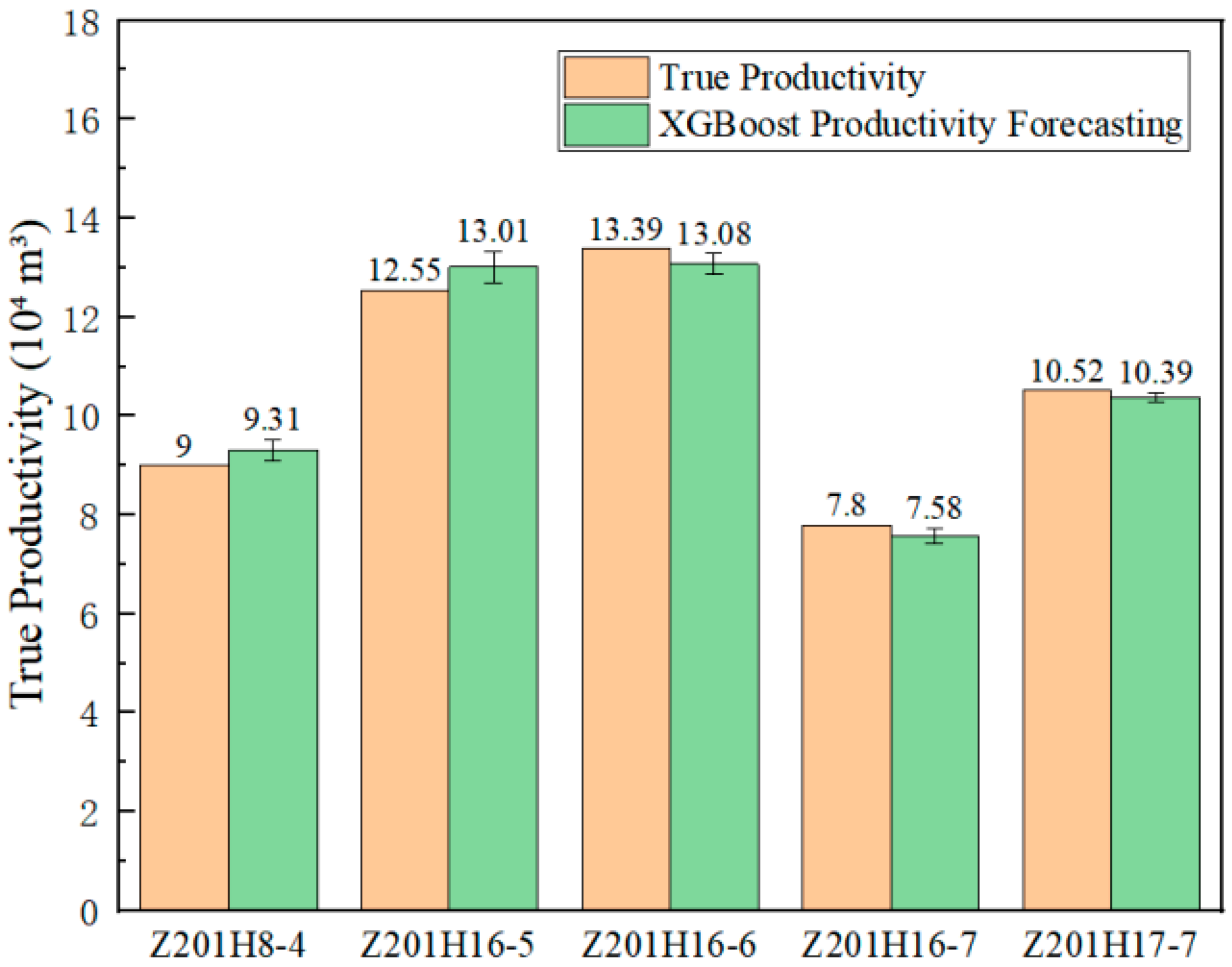
For engineering validation, the trained XGBoost productivity prediction model was applied to the Z201 Block. As shown in Figure 10, the prediction errors against the actual productivity consistently remained below 5%. The model further predicted stabilized gas rates for wells lacking production data in the Z201 Block of the Western Chongqing Gas Field, providing critical data support for subsequent reservoir development.
The validation and application of the model deliberately focused on the Zu201 Block (as shown in Figure 12) for two primary reasons. Firstly, as the most actively developed block in the Western Chongqing area with ongoing production, it represents the most critical and practical scenario for applying the predictive model to guide immediate development decisions. Secondly, wells from the Zu203 and Zu206 Blocks were included in the training dataset to enhance the model’s general understanding of geological and engineering patterns across the entire region. While this incorporation strengthens the overall model robustness, it precludes their use for independent validation, as they are not “unseen” data.
However, the performance on the Zu201 Block alone cannot fully represent the model’s generalizability to entirely new blocks with potentially different geological characteristics. This deliberate focus highlights a key limitation and, concurrently, a clear direction for future work: the application and validation of this interpretable ML framework to newly discovered or developing blocks (e.g., Zu203, Zu206, or other future blocks) once sufficient production data from wells that were not part of this study’s training set becomes available. Such research would be invaluable for testing the true transferability of the model and for refining it to become a universal tool for shale gas productivity prediction in the Sichuan Basin.
The data analysis and machine learning modeling were conducted entirely in Python (version 3.12.7). The following key libraries were utilized: scikit-learn (v1.5.1) for the implementation of Random Forest and Support Vector Machine algorithms, pandas (v2.2.2) for data manipulation, XGBoost (v2.1.1) for gradient boosting, and SHAP (v0.47.2) for model interpretation. Numerical computations were supported by NumPy (v1.26.4) and SciPy (v1.13.1), while Matplotlib (v3.9.2) was used for visualization.

3.4. Analysis Results of the Main Control Factors

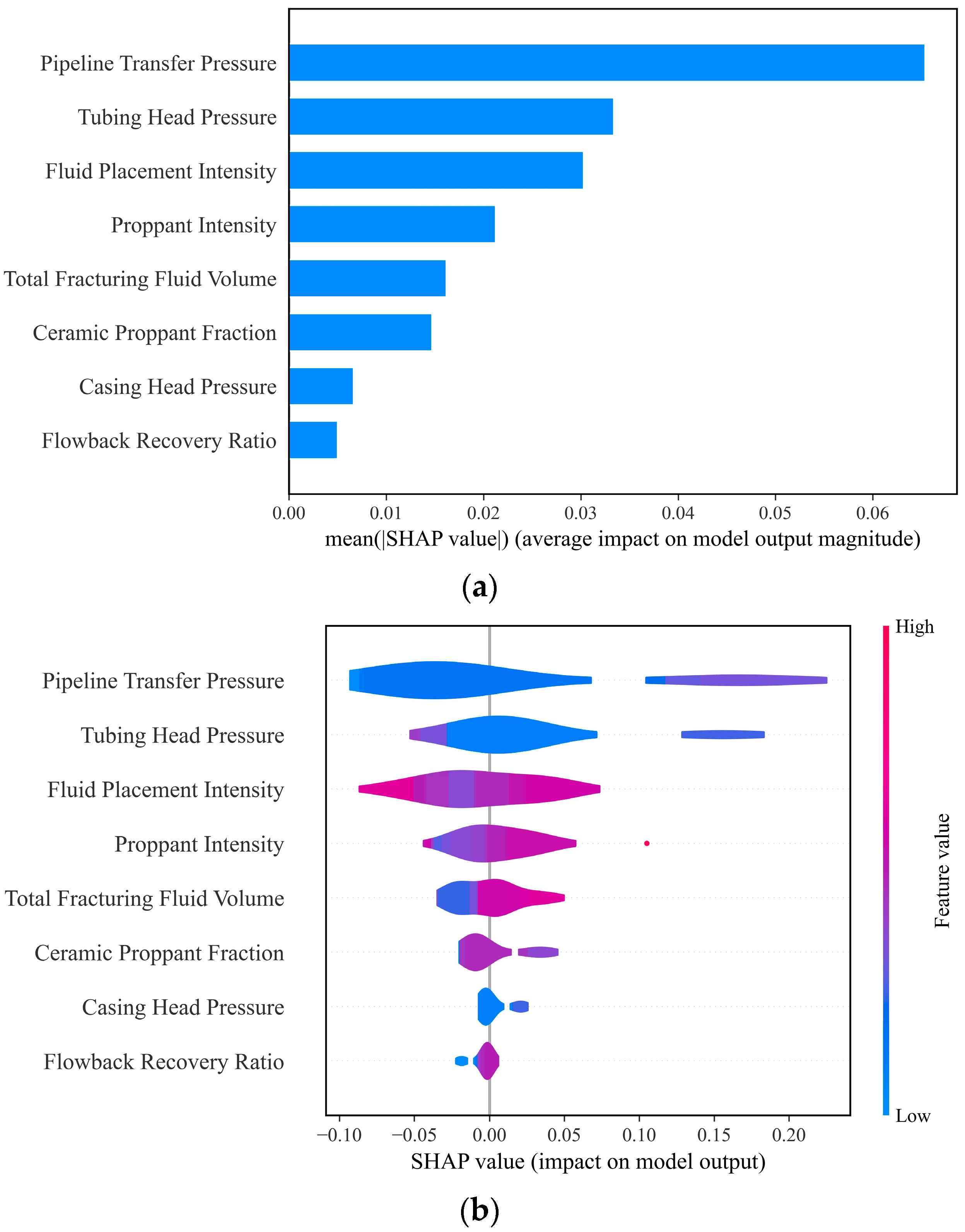
Leveraging the superior prediction performance of the XGBoost model, SHAP (SHapley Additive exPlanations) interpretability analysis was employed to elucidate the influence mechanisms of different features on gas well productivity and decipher the model’s decision logic. As illustrated in Figure 13, we utilized three complementary visualization techniques: (a) feature global importance ranking, quantifying the relative contribution strength of each feature; (b) beeswarm plots, identifying nonlinear effects (e.g., threshold behaviors) in continuous features; and (c) dependence plots, characterizing the direction and magnitude of influence of individual features [47,48,49,50,51].
The feature importance plot (Figure 13a) provides a global interpretation of the XGBoost model, indicating that tubing head pressure and pipeline transfer pressure are the two most influential features with significant impacts on productivity predictions. Additionally, parameters including ceramic proppant fraction, proppant intensity, total fracturing fluid volume, and fluid placement intensity substantially affect model outputs, albeit to a lesser degree.
The beeswarm plot (Figure 13b) visualizes the distribution of the SHAP values for each feature, where the individual points represent fractured horizontal wells. The point colors encode feature values on a blue-to-red scale (low to high). Crucially, SHAP values quantify feature contributions to model predictions: positive values increase predicted productivity, while negative values decrease it. For instance, tubing head pressure exhibits widely dispersed SHAP values, confirming its significant influence. Analysis of ceramic proppant fraction reveals distinct patterns: high fractions (red) consistently decrease the predicted productivity, whereas low fractions (blue) increase it in this dataset.
The dependence plot (Figure 13c) integrates SHAP value distributions with feature magnitudes to visualize each feature’s influence on model predictions. Each point represents the SHAP value of a shale gas well sample, with the point distribution indicating the feature’s effect range across wells. The features are ranked in descending order of their average impact magnitude. A concentrated SHAP value distribution denotes consistent effects across samples, whereas dispersion reflects variability—as demonstrated by casing head pressure’s tightly clustered SHAP values, indicating highly consistent impacts. Subsequent analysis will quantify the effects of key parameters on productivity based on these findings.
Crucially, the synergy between these plots reveals a coherent and mechanistically sound narrative. The high global ranking of tubing head pressure and pipeline transfer pressure in the summary plot (Figure 13a) is a direct consequence of the strong, consistent positive relationships exhibited in their dependence plots (as exemplified in Figure 13b,c for these specific features).
This positive correlation signifies that higher values of these pressure parameters universally contribute to increased predicted gas production across the dataset. This finding aligns perfectly with fundamental petroleum engineering principles, where higher wellhead and pipeline pressures are indicative of greater reservoir energy and driving force, which are primary controllers of flow rate. Therefore, the SHAP analysis identifies statistically important features and also successfully uncovers the underlying physical drivers of shale gas productivity, with reservoir and flowline pressure being the most dominant factors in this study.

3.5. Parameter Sensitivity Analysis

To quantify the impact of individual engineering parameter variations on shale gas well production capacity and clarify their respective effects, we introduce the average production capacity elasticity coefficient (E). This approach builds upon a trained XGBoost model and SHAP analysis, applying the finite-difference perturbation method based on its underlying principle:
E = Δ Q / Q Δ P / P
where Δ Q / Q is the rate of change in production capacity and Δ P / P is the rate of change in the corresponding parameter. Classified by |E| > 0.5 (strong elasticity), 0.3 ≤ |E| ≤ 0.5 (medium elasticity), and |E| < 0.3 (weak elasticity), a single-parameter perturbation analysis was carried out based on the already-trained model, where a systematic parameter perturbation analysis was used to quantitatively assess the sensitivity effects of the fracturing construction parameters on capacity.
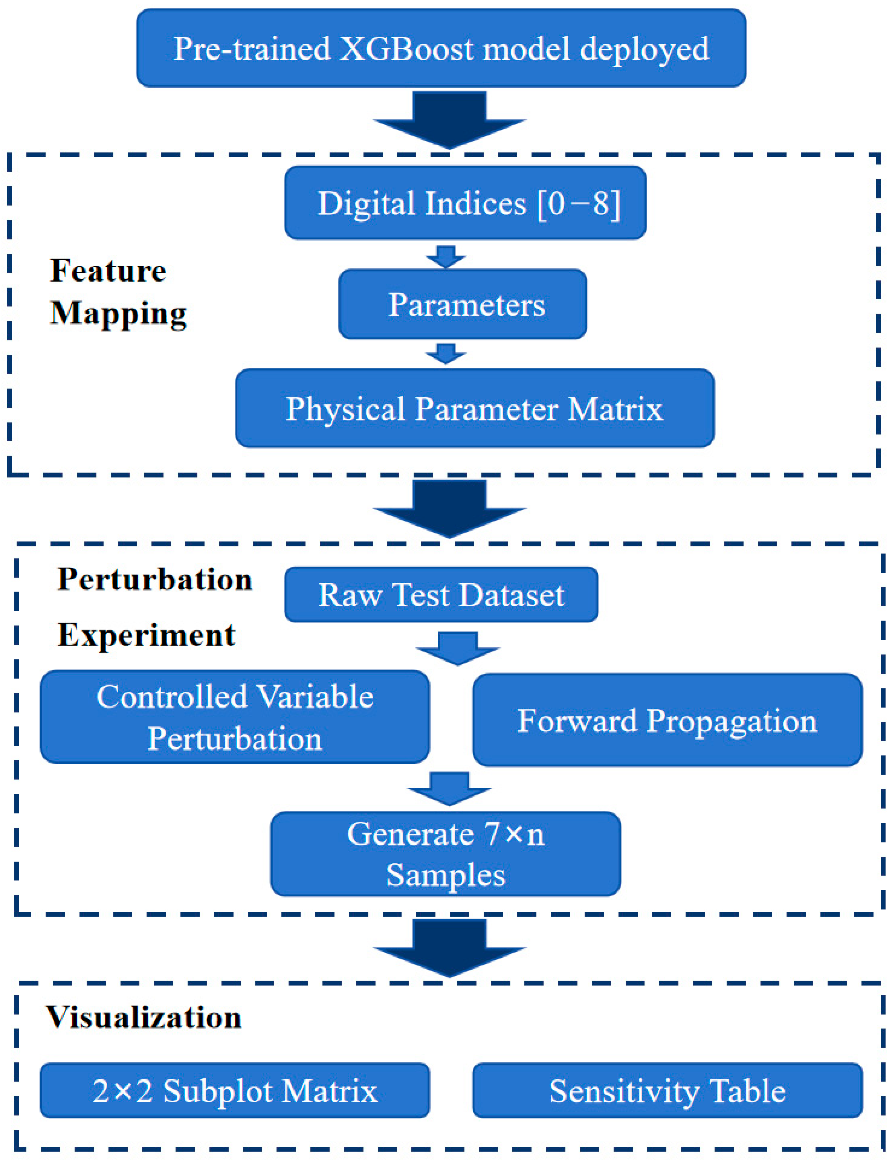
Firstly, a feature mapping mechanism was used to convert numerical indices 0–8 into physically meaningful engineering parameters (e.g., ceramic proppant fraction, proppant intensity), establishing parameter–productivity correlations. Using the test set data as the baseline, a controlled variable perturbation strategy was implemented: seven equidistant points within ±15% variation were generated for each target parameter. Forward propagation through the model was used to compute productivity change rates (ΔQ/Q), avoiding multicollinearity interference. Finally, the sensitivity results were visualized bi-dimensionally via a 2 × 2 subplot matrix, displaying the perturbation–response curves of key parameters. The axes show standardized percentage change rates with zero-reference baselines. Sensitivity was quantified via elasticity coefficients (Table 5), delivering quantitative decision support for fracturing parameter optimization.
The specific process is shown below (Figure 14):
A sensitivity analysis of fracturing parameters was conducted in this study using the elasticity coefficient E (Table 8), leading to the proposal of a control strategy. The parameters were classified into high-sensitivity (|E| > 0.5) and low-sensitivity (|E| < 0.3) categories, with tailored control measures developed for each group.
The high-sensitivity parameters, such as total fracturing fluid volume and proppant intensity, constitute the primary control targets, with sensitivity charts allowing for optimization within economic ranges. The low-sensitivity parameters, like ceramic proppant fraction, were treated as cost-control levers. Since these parameters minimally impact productivity, cost factors dominate their adjustment strategies.
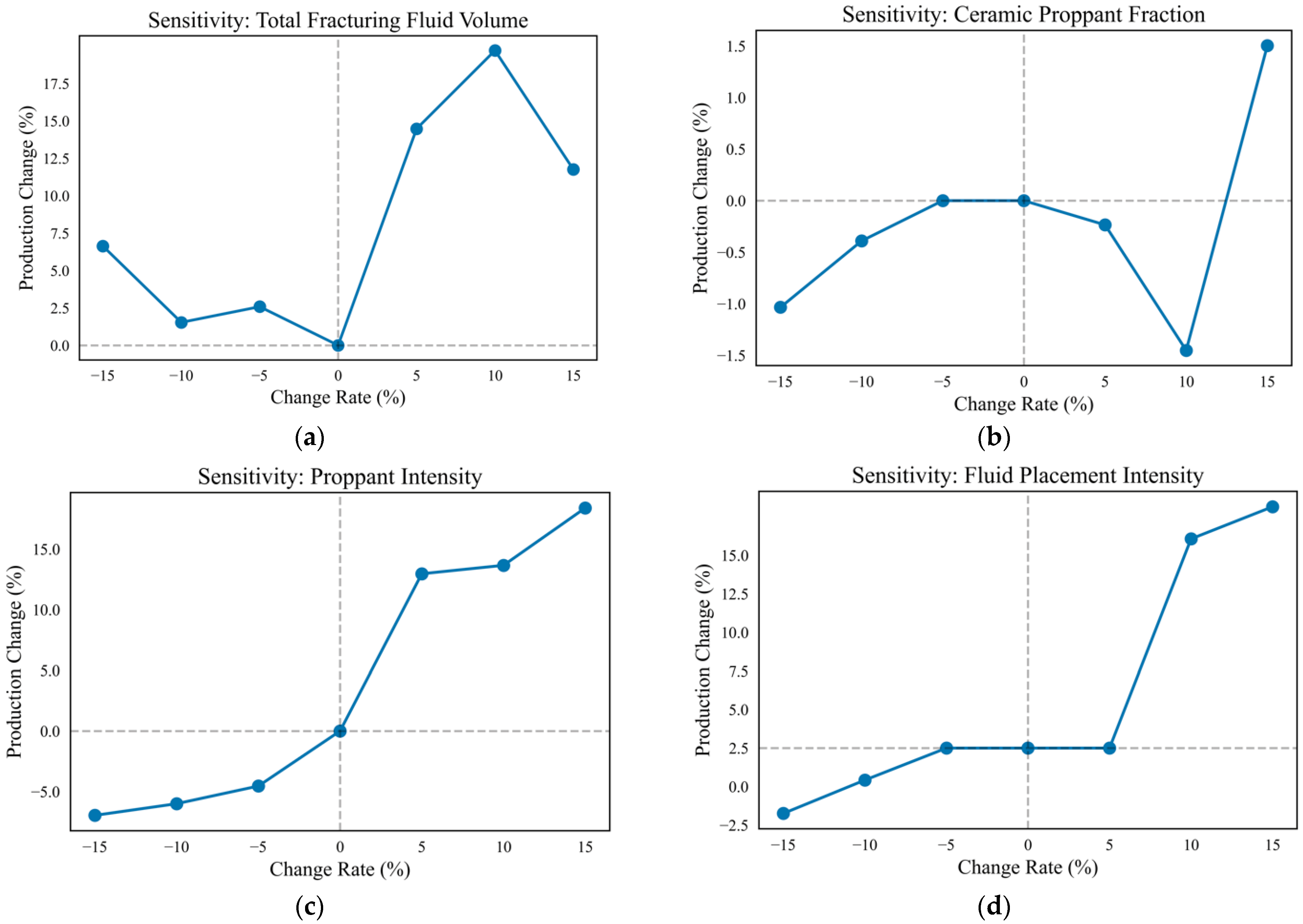
This analysis reveals the nonlinear influences of the parameters on productivity by examining the sensitivity curve morphologies and elasticity coefficients, providing a theoretical basis for optimizing field operation parameters. An analysis of the elasticity coefficients reveals the following (Figure 15): Figure 15a shows that productivity initially increases and then declines with rising total fracturing fluid volume. Within the +10% perturbation range, productivity increases by 7.3% on average (elasticity coefficient E = 0.73), classifying it as a strongly elastic parameter. However, exceeding a +15% volume increase yields diminishing returns, indicating an economically optimal range. Based on the test set data, we recommend maintaining the fluid volume at 70,000–85,000 m3 (corresponding to +5% to +10% perturbation) for maximal efficiency. Figure 15b demonstrates that ceramic proppant fraction has an inverted U-shaped impact on productivity, peaking at the current baseline (0% perturbation). Near +10% perturbation, productivity declines significantly, suggesting critical sensitivity. An optimal proppant fraction should be controlled within 40–45%, avoiding drastic adjustments to prevent productivity loss.
For proppant intensity (Figure 15c), productivity increases quasi-linearly with intensity, reflected in a high elasticity coefficient (E > 0.8), confirming strong elasticity. The plateau inflection at +5% to +10% perturbation supports optimization to 4.23–4.43 t/m.
Figure 15d indicates that fluid placement intensity has minimal impact below +5% perturbation but triggers steep productivity increases beyond this threshold (elasticity E = 0.6 per 1% intensity increase above +10%). Considering formation fracture pressure limits, we recommend maintaining a proppant intensity of 41.86–43.06 m3/m (a +5% to +8% perturbation) to enhance productivity while preventing excessive fracture interference.
These recommended optimal ranges are derived from and supported by the response of the 15-well test set, which serves as a representative validation subset of the Western Chongqing Block. The sensitivity curves in Figure 15, therefore, represent the aggregate and consistent response of this entire hold-out well group to parameter perturbations, ensuring that the recommendations are robust and not unduly influenced by individual outliers.
For instance, the key recommendation for total fracturing fluid volume (70,000–85,000 m3) is substantiated by the fact that most of the test set wells exhibit their peak or near-peak productivity within this range. Similarly, the inflection points and trends observed for other parameters (e.g., the plateau for proppant intensity, the threshold for fluid placement intensity) are consistently demonstrated across this group of wells.

4. Conclusions

To address productivity prediction challenges arising from complex geological–engineering conditions and strong coupling in Western Chongqing’s deep shale gas wells, this study integrates gray relational analysis with three interpretable machine learning techniques (SVM, RF, XGBoost). Eight engineering master control parameters—including total fracturing fluid volume and proppant intensity—were optimized to establish a small-sample-based intelligent productivity prediction and operational parameter optimization framework. Systematic analysis of 87 gas wells yields the following conclusions:
  • Through model training, parameter optimization, and cross-validation, this study confirmed XGBoost’s superior performance with a test set R2 of 0.907, representing 12.11% and 131.38% improvements over RF and SVR, respectively. The model achieved significantly lower error metrics: RMSE (0.06393) decreased by 30.1% vs. RF and 60.8% vs. SVR; MAE (0.05059) decreased by 21.7% and 52.2% compared to RF and SVR; and MSE (0.00409) decreased by 51.1% and 84.6% compared to RF and SVR, demonstrating comprehensive prediction accuracy advantages. The comparative analysis conclusively demonstrated that the XGBoost model significantly outperformed both the Random Forest and Support Vector Machine models, establishing it as the most effective tool for productivity prediction under the studied conditions. The field validation in the Western Chongqing Gas Field maintained productivity prediction errors consistently below 5%, fulfilling real-time engineering decision-making requirements.
  • Gray relational analysis further confirmed the dominant influence of dynamic parameters like pipeline transfer pressure and average tubing head pressure on productivity. Global sensitivity analysis via SHAP interpretability revealed pressure parameters as primary drivers (|mean SHAP| ≈ 0.045), significantly outperforming ceramic proppant fraction (|mean SHAP| ≈ 0.025). Mechanistically, elevated ceramic proppant fraction moderately enhanced productivity but remained weaker than pressure effects; proppant intensity exhibited threshold behavior requiring avoidance of low-value negative-impact zones; and fluid placement intensity showed diminishing marginal returns at high values. Consequently, engineering optimization should prioritize pressure parameter adjustment, target optimal proppant intensity thresholds, and treat ceramic proppant fraction as a secondary adjustment parameter.
  • Based on the test set well group sensitivity analysis, total fracturing fluid volume and proppant intensity were identified as strongly elastic parameters (|E| > 0.5), requiring priority optimization within the economic range (+5%~+10%). Weakly elastic parameters like ceramic proppant fraction (|E| < 0.3) should undergo narrow-window control (−3%~+2%) for cost efficiency. This establishes a tiered control strategy for deep shale gas development in the Western Chongqing Block: the primary focus should be on economically optimizing strongly elastic parameters, followed by the secondary stabilization of weakly elastic parameters. The model enables well-specific customization, allowing future sensitivity analyses and parameter optimization designs for individual wells in the block. It is important to note that the present sensitivity analysis evaluates the impact of varying one parameter while holding the others constant. Future work could employ more advanced global sensitivity analysis techniques (e.g., Sobol indices) to explore interaction effects between parameters and to identify the most influential parameter combinations under different geological and operational scenarios.
  • This study establishes an interpretable ML framework that delivers robust predictions of key shale gas development indicators for the Western Chongqing Block. The model’s primary immediate application is in field-scale development planning, providing data-driven guidance on overall stimulation design and well spacing based on global sensitivity analysis. The practical guidelines outlined in Section 3.5 provide a clear pathway for deploying this methodology elsewhere, emphasizing the necessity of local calibration. A critical finding is that, while the current model offers block-level optimization advice, the transition to single-well customized optimization presents a compelling frontier. Our future research will therefore focus on adapting this framework to generate well-specific sensitivity analyses, ultimately moving towards a truly digital twin solution for shale gas development that can provide tailored engineering recommendations for every individual well.

Author Contributions

Conceptualization and methodology, H.Z.; data processing, Y.Z.; investigation and validation, Y.L.; supervision and writing—review and editing, C.S.; writing—review and editing, W.C. and D.Z. All authors have read and agreed to the published version of the manuscript.

Funding

This research was funded by the Natural Science Foundation of Sichuan Province, grant number 2024NSFSC2019.

Data Availability Statement

The datasets generated and analyzed during the current study are not publicly available due to the ongoing nature of the research and confidentiality agreements related to the developing block. However, they are available from the corresponding author on reasonable request for academic collaboration, subject to approval by the project partners.

Conflicts of Interest

The authors declare that Haijie Zhang, Chaoya Sun, and Weiming Ming are employed by Chongqing Shale Gas Exploration and Development Co., Ltd. This may lead to a potential conflict of interest regarding the research work reported in this paper. The funders had no role in the design of the study; in the collection, analyses, or interpretation of data; in the writing of the manuscript; or in the decision to publish the results.

References

  1. Zhou, W.; Zhu, J.; Wang, H.; Kong, D. Transport Diffusion Behaviors and Mechanisms of CO2/CH4 in Shale Nanopores: Insights from Molecular Dynamics Simulations. Energy Fuels 2022, 36, 11903–11912. [Google Scholar] [CrossRef]
  2. Zhao, Y.-L.; Li, N.-Y.; Zhang, L.-H.; Zhang, R.-H. Productivity analysis of a fractured horizontal well in a shale gas reservoir based on discrete fracture network model. J. Hydrodyn. 2019, 31, 552–561. [Google Scholar] [CrossRef]
  3. Luo, G.; Tian, Y.; Bychina, M.; Ehlig-Economides, C. Production Optimization Using Machine Learning in Bakken Shale. In Proceedings of the SPE/AAPG/SEG Unconventional Resources Technology Conference, Houston, TX, USA, 23–25 July 2018; OnePetro: Houston, TX, USA, 2018; p. URTEC-2902505-MS. [Google Scholar]
  4. Wang, K.; Li, H.; Wang, J.; Jiang, B.; Bu, C.; Zhang, Q.; Luo, W. Predicting Production and Estimated Ultimate Recoveries for Shale Gas Wells: A New Methodology Approach. Appl. Energy 2017, 206, 1416–1431. [Google Scholar] [CrossRef]
  5. Fang, X.; Yue, X.; An, W.; Feng, X. Experimental Study of Gas Flow Characteristics in Micro-/Nano-Pores in Tight and Shale Reservoirs Using Microtubes under High Pressure and Low Pressure Gradients. Microfluid. Nanofluid. 2019, 23, 5. [Google Scholar] [CrossRef]
  6. Pang, W.; Du, J.; Zhang, T. Production Data Analysis of Shale Gas Wells with Abrupt Gas Rate or Pressure Changes. In Proceedings of the SPE Middle East Oil and Gas Show and Conference, Manama, Bahrain, 15–21 March 2019; p. D041S046R001. [Google Scholar]
  7. Zhou, Y.; Gu, Z.; He, C.; Yang, B.; Xiong, J. Analysis of Influencing Factors on Shale Gas Well Productivity based on Random Forest. Int. J. Energy 2025, 6, 37–46. [Google Scholar] [CrossRef]
  8. Wang, M.; He, J.; Liu, S.; Zeng, C.; Jia, S.; Nie, Z.; Zhang, C. Effect of sedimentary facies characteristics on deep shale gas desserts: A case from the Longmaxi Formation, South Sichuan Basin, China. Minerals 2023, 13, 476. [Google Scholar] [CrossRef]
  9. Li, J.; Zeng, X.; Lian, C.; Lin, H.; Liu, S.; Lei, F.; Wan, Y. Research on the comprehensive dessert evaluation method in shale oil reservoirs based on fractal characteristics of conventional logging curves. Sci. Rep. 2025, 15, 9318. [Google Scholar] [CrossRef]
  10. Jiang, M.; Peng, C.; Wu, J.; Wang, Z.; Liu, Y.; Zhao, B.; Zhang, Y. A New Approach to a Fracturing Sweet Spot Evaluation Method Based on Combined Weight Coefficient Method—A Case Study in the BZ Oilfield, China. Processes 2024, 12, 1830. [Google Scholar] [CrossRef]
  11. Liu, S.; Wang, M.; Cheng, Y.; Yu, X.; Duan, X.; Kang, Z.; Xiong, Y. Fractal insights into permeability control by pore structure in tight sandstone reservoirs, Heshui area, Ordos Basin. Open Geosci. 2025, 17, 20250791. [Google Scholar] [CrossRef]
  12. Stalgorova, E.; Mattar, L. Analytical Model for History Matching and Forecasting Production in Multifrac Composite Systems. In Proceedings of the SPE Canada Unconventional Resources Conference, Calgary, AL, Canada, 30 October–1 November 2012; p. SPE-162516-MS. [Google Scholar]
  13. Du, F.; Huang, J.; Chai, Z.; Killough, J. Effect of Vertical Heterogeneity and Nano-Confinement on the Recovery Performance of Oil-Rich Shale Reservoir. Fuel 2020, 267, 117199. [Google Scholar] [CrossRef]
  14. Huang, S.; Ding, G.; Wu, Y.; Huang, H.; Lan, X.; Zhang, J. A Semi-Analytical Model to Evaluate Productivity of Shale Gas Wells with Complex Fracture Networks. J. Nat. Gas Sci. Eng. 2018, 50, 374–383. [Google Scholar] [CrossRef]
  15. Lin, X.; Floudas, C.A. A Novel Continuous-Time Modeling and Optimization Framework for Well Platform Planning Problems. Optim. Eng. 2003, 4, 65–95. [Google Scholar] [CrossRef]
  16. Rumelhart, D.E.; Hinton, G.E.; Williams, R.J. Learning representations by back-propagating errors. Nature 1986, 323, 533–536. [Google Scholar] [CrossRef]
  17. Meng, M.; Zhao, C. Application of Support Vector Machines to a Small-Sample Prediction. Adv. Pet. Explor. Dev. 2015, 10, 72–75. [Google Scholar] [CrossRef]
  18. Hui, G.; Chen, S.; He, Y.; Wang, H.; Gu, F. Machine Learning-Based Production Forecast for Shale Gas in Unconventional Reservoirs via Integration of Geological and Operational Factors. J. Nat. Gas Sci. Eng. 2021, 94, 104045. [Google Scholar] [CrossRef]
  19. Song, L.; Wang, C.; Lu, C.; Yang, S.; Tan, C.; Zhang, X. Machine Learning Model of Oilfield Productivity Prediction and Performance Evaluation. J. Phys. Conf. Ser. 2023, 2468, 012084. [Google Scholar] [CrossRef]
  20. Rahmanifard, H.; Gates, I.D. Innovative integrated workflow for data-driven production forecasting and well completion optimization: A Montney Formation case study. Geoenergy Sci. Eng. 2024, 238, 212899. [Google Scholar] [CrossRef]
  21. Guan, W.; Peng, X.; Zhu, S.; Yang, C.; Peng, Z.; Ma, X. Research on productivity prediction method of infilling well based on improved LSTM neural network: A case study of the middle-deep shale gas in South Sichuan. Pet. Reserv. Eval. Dev. 2025, 15, 479–487. [Google Scholar] [CrossRef]
  22. Wang, S.; Chen, S. Insights to fracture stimulation design in unconventional reservoirs based on machine learning modeling. J. Pet. Sci. Eng. 2019, 174, 682–695. [Google Scholar] [CrossRef]
  23. Zhou, X.; Ran, Q. Production prediction based on ASGA-XGBoost in shale gas reservoir. Energy Explor. Exploit. 2024, 42, 462–475. [Google Scholar] [CrossRef]
  24. Guevara, J.; Zadrozny, B.; Buoro, A.; Tolle, J.; Limbeck, J.; Wu, M.; Hohl, D. An Interpretable Machine Learning Methodology for Well Data Integration and Sweet Spotting Identification; NIPS 2018 Workshop Book; HAL: Montreal, QC, Canada, 2018; p. Hal-02199055. [Google Scholar]
  25. Liu, H.-H.; Zhang, J.; Liang, F.; Temizel, C.; Basri, M.A.; Mesdour, R. Incorporation of physics into machine learning for production prediction from unconventional reservoirs: A brief review of the gray-box approach. SPE Reserv. Eval. Eng. 2021, 24, 847–858. [Google Scholar] [CrossRef]
  26. Castro, M.; Mendes Júnior, P.R.; Soriano-Vargas, A.; de Oliveira Werneck, R.; Gonçalves, M.M.; Filho, L.L.; Moura, R.; Zampieri, M.; Linares, O.; Ferreira, V.; et al. Time series causal relationships discovery through feature importance and ensemble models. Sci. Rep. 2023, 13, 11402. [Google Scholar] [CrossRef]
  27. Syed, F.I.; Alnaqbi, S.; Muther, T.; Dahaghi, A.K.; Negahban, S. Smart shale gas production performance analysis using machine learning applications. Pet. Res. 2022, 7, 21–31. [Google Scholar] [CrossRef]
  28. Dong, Y.; Qiu, L.; Lu, C.; Song, L.; Ding, Z.; Yu, Y.; Chen, G. A data-driven model for predicting initial productivity of offshore directional well based on the physical constrained eXtreme gradient boosting (XGBoost) trees. J. Pet. Sci. Eng. 2022, 211, 110176. [Google Scholar] [CrossRef]
  29. Ma, K.; Wu, C.; Huang, Y.; Mu, P.; Shi, P. Oil well productivity capacity prediction based on support vector machine optimized by improved whale algorithm. J. Pet. Explor. Prod. Technol. 2024, 14, 3251–3260. [Google Scholar] [CrossRef]
  30. Li, J.-H.; Ji, L. Productivity forecast for multi-stage fracturing in shale gas wells based on a random forest algorithm. Energy Sources Part A Recovery Util. Environ. Eff. 2025, 47, 2834–2843. [Google Scholar] [CrossRef]
  31. GB/T 41612-2022; Technical Specifications for Shale Gas Well Production Prediction. Standard Press of China: Beijing, China, 2022. (In Chinese)
  32. NB/T 14024-2017; Technical Specifications for Shale Gas Well Production Prediction. National Energy Administration: Beijing, China, 2017.
  33. Abbas, K.; Jiahua, C.; Shili, L. Feature selection in finite mixture of sparse normal linear models in high-dimensional feature space. Biostatistics 2011, 12, 156–172. [Google Scholar] [CrossRef]
  34. Yu, L.; Liu, H. Efficient feature selection via analysis of relevance and redundancy. J. Mach. Learn. Res. 2004, 5, 1205–1224. [Google Scholar]
  35. King, G.E. Thirty Years of Gas Shale Fracturing: What Have We Learned? SPE Annual Technical Conference and Exhibition. In Proceedings of the SPE Annual Technical Conference and Exhibition, Florence, Italy, 19–22 September 2010; p. SPE-133456-MS. [Google Scholar]
  36. Wang, X.; Fang, H.; Fang, S. An integrated approach for exploitation block selection of shale gas—Based on cloud model and grey relational analysis. Resour. Policy 2020, 68, 101797. [Google Scholar] [CrossRef]
  37. Lozng, Z.L.; Wen, Z.T.; Li, H.; Zeng, X. An evaluation method of shale reservoir crushability based on grey correlation analysis. Reserv. Eval. Dev. 2020, 10, 37–42. [Google Scholar] [CrossRef]
  38. Aili, Q. Grey Relational Analysis on Elderly People’ Life Quality and Sports. Res. J. Appl. Sci. Eng. Technol. 2013, 6, 63–69. [Google Scholar] [CrossRef]
  39. Xiao, H. Production evaluation method based on grey correlation analysis for shale gas horizontal wells in Weiyuan block. Well Test. 2018, 27, 73–78. [Google Scholar]
  40. Chen, D.; Tan, Z.; Wu, L.; Xia, L.; Li, H.; Zhao, Y. Method of low-permeability reservoir productivity evaluation while drilling based on grey correlation analysis of logging parameters. Mud Logging Eng. 2025, 36, 34–40+55. [Google Scholar]
  41. Buchanan, J.W.; Ali, H. Evaluation of Privacy-Preserving Support Vector Machine (SVM) Learning Using Homomorphic Encryption. Cryptography 2025, 9, 33. [Google Scholar] [CrossRef]
  42. Ignatenko, V.; Surkov, A.; Koltcov, S. Random forests with parametric entropy-based information gains for classification and regression problems. PeerJ. Comput. Sci. 2024, 10, e1775. [Google Scholar] [CrossRef]
  43. Mohammadian, E.; Kheirollahi, M.; Liu, B.; Ostadhassan, M.; Sabet, M. A case study of petrophysical rock typing and permeability prediction using machine learning in a heterogenous carbonate reservoir in Iran. Sci. Rep. 2022, 12, 4505. [Google Scholar] [CrossRef] [PubMed]
  44. Wu, L.; Li, J.; Ma, D.; Wang, Z.; Zhang, J.; Yuan, C.; Feng, Y.; Li, H. Prediction for Rock Compressive Strength Based on Ensemble Learning and Bayesian Optimization. Earth Sci. 2023, 48, 1686–1695. [Google Scholar] [CrossRef]
  45. Lundberg, S.; Lee, S.-I. A Unified Approach to Interpreting Model Predictions. arXiv 2017, arXiv:1705.07874. [Google Scholar] [CrossRef]
  46. Lundberg, S.M.; Erion, G.; Chen, H.; DeGrave, A.; Prutkin, J.M.; Nair, B.; Katz, R.; Himmelfarb, J.; Bansal, N.; Lee, S.-I. From Local Explanations to Global Understanding with Explainable AI for Trees. Nat. Mach. Intell. 2020, 2, 56–67. [Google Scholar] [CrossRef]
  47. Oona, R.; Jarmo, T.; Riku, K. Evaluation metrics and statistical tests for machine learning. Sci. Rep. 2024, 14, 6086. [Google Scholar] [PubMed]
  48. Song, Y.; Zhu, Y.; Zeng, B. Efficient Identification Method of Interbeds Based on Neural Network Combined with Grey Relational Analysis—Taking the Lower Sub-Member of the Sangonghe Formation in Moxizhuang Oilfield as an Example. J. Geosci. Environ. Prot. 2025, 13, 51–68. [Google Scholar] [CrossRef]
  49. Raheem, O.; Morales, M.M.; Pan, W.; Torres-Verdín, C. Improved estimation of two-phase capillary pressure with nuclear magnetic resonance measurements via machine learning. Artif. Intell. Geosci. 2025, 6, 100144. [Google Scholar] [CrossRef]
  50. Zhang, T.; Peng, F.; Yan, R.; Tang, X.; Yuan, J.; Deng, R. An uncertainty quantification and accuracy enhancement method for deep regression prediction scenarios. Mech. Syst. Signal Process. 2025, 227, 112394. [Google Scholar] [CrossRef]
  51. Chen, R.; Liu, X.; Zhou, S.; Zhang, W.; Liu, H.; Yan, D.; Wang, H. Application of machine learning model in shale TOC content prediction based on well log data: Enhancing model interpretability by SHAP. Earth Sci. Inform. 2025, 18, 428. [Google Scholar] [CrossRef]
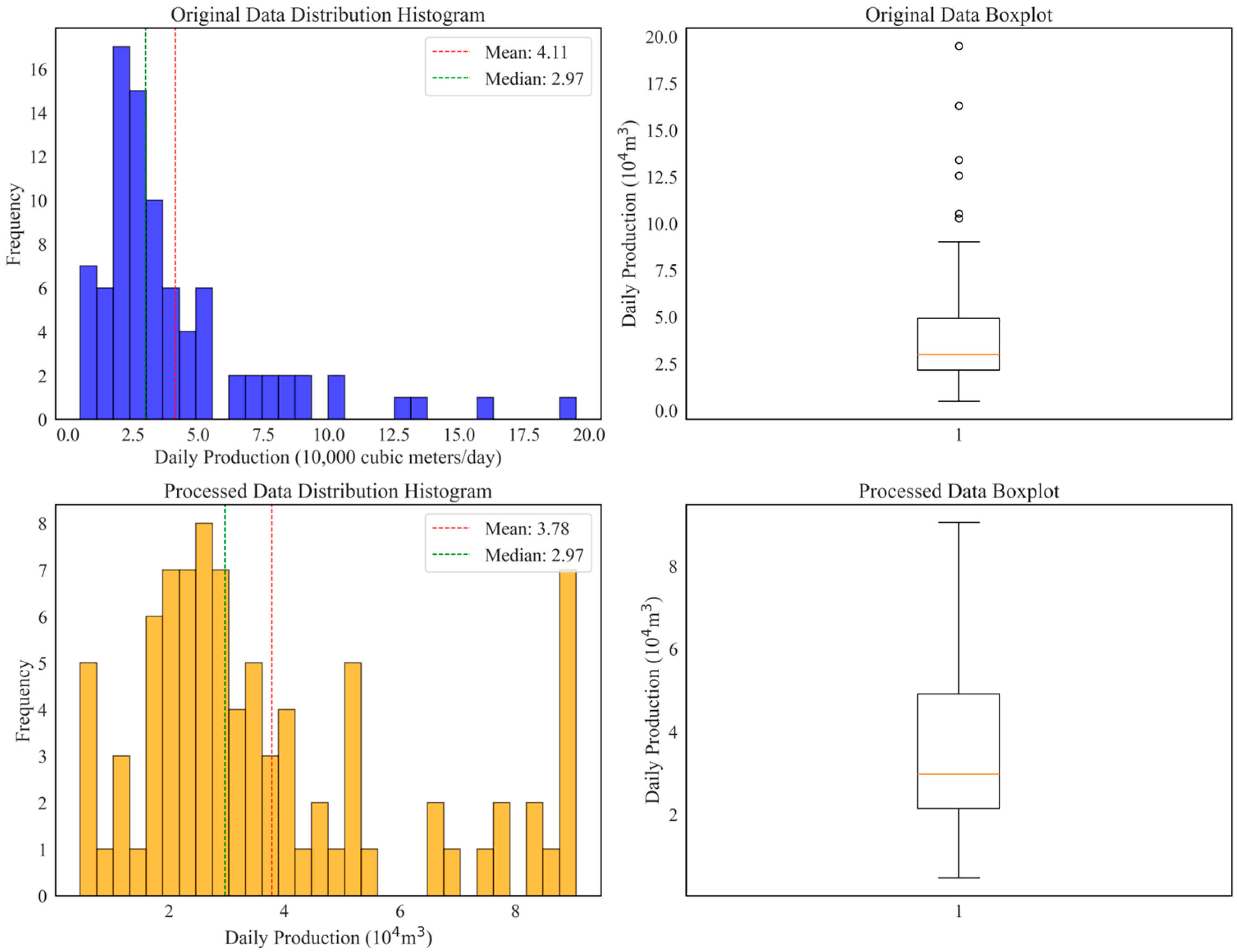
Figure 1. Distribution comparison of daily gas production before and after outlier treatment. The histogram illustrates the distribution transformation; the boxplot illustrates the dispersion improvement. For the 87 samples, minor data gaps (<5% missing rate) in variables, like casing head pressure and proppant intensity, were addressed with median imputation (Table 2). The dataset was partitioned into training (80%) and test (20%) subsets.
Processes 13 03279 g001
Figure 2. Heatmap of gray relational analysis for dominant controlling factors of shale gas productivity.
Processes 13 03279 g002
Figure 3. Gray relational matrix of dominant controlling factors for shale gas productivity.
Processes 13 03279 g003
Figure 4. Mechanism schematic of support vector regression.
Processes 13 03279 g004
Figure 5. Workflow of the random forest algorithm construction. Arrows show the aggregation of predictions from all trees. Orange circles mark the classification path taken by each tree for the given instance. The “Training Voting” module illustrates the majority voting mechanism that combines all tree outputs to determine the final predicted class.
Processes 13 03279 g005
Figure 6. Computational workflow of boosting ensemble algorithms. Rectangular boxes represent individual weak learners (decision trees). Arrows indicate the sequential flow of data and residual corrections. Orange circles highlight the specific path (tree branch) selected for the given instance at each stage. The “Sum” operation denotes the additive combination of all tree predictions to generate the final result.
Processes 13 03279 g006
Figure 7. Flowchart for machine learning model training and optimization.
Processes 13 03279 g007
Figure 8. Test set scatter plots: predicted vs. measured productivity across models. (a1) SVR training set capacity prediction regression curve; (a2) SVR testing set capacity prediction regression curve; (b1) RF training set capacity prediction regression curve; (b2) RF testing set capacity prediction regression curve; (c1) XGBoost training set capacity prediction regression curve; (c2) XGBoost testing set capacity prediction regression curve.
Processes 13 03279 g008
Figure 9. Comparative performance metrics of models.
Processes 13 03279 g009
Figure 10. Error distribution curves for productivity forecasting. (a) SVR gas well production prediction error curve; (b) RF gas well production prediction error curve; (c) XGBoost gas well production prediction error curve.
Processes 13 03279 g010
Figure 11. Model performance comparison: five-fold cross-validation R2 score analysis. (a) Box plots comparing the distribution of five-fold cross-validation R2 scores for three machine learning models (SVM, Random Forest, XGBoost). Statistical tests indicate highly significant performance differences among the models (F = 127.47, p < 0.001). (b) Enhanced box plots with 95% confidence intervals, providing additional evidence for the superiority of XGBoost in terms of prediction stability and reliability.
Processes 13 03279 g011
Figure 12. XGBoost-based productivity prediction for the Z201 Block of the Western Chongqing Gas Field.
Processes 13 03279 g012
Figure 13. SHAP-based interpretability analysis for the XGBoost productivity prediction model. (a) feature global importance ranking, quantifying the relative contribution strength of each feature; (b) beeswarm plots, identifying nonlinear effects (e.g., threshold behaviors) in continuous features; and (c) dependence plots, characterizing the direction and magnitude of influence of individual features.
Processes 13 03279 g013aProcesses 13 03279 g013b
Figure 14. Workflow diagram for parameter sensitivity analysis model construction.
Processes 13 03279 g014
Figure 15. Parameter–productivity sensitivity curves. (a) Total fracturing fluid volume; (b) Ceramic proppant fraction; (c) Proppant intensity; (d) Fluid placement intensity.
Processes 13 03279 g015
Table 1. Description of input variables for shale gas well productivity prediction.
Feature NamePhysical SignificanceUnit
Proppant IntensityProppant injection per unit layer thicknesst/m
Ceramic Proppant FractionMass fraction of ceramic sand in total proppant%
Fluid Placement IntensityFracturing fluid injection volume per unit thickness of formationm3/m
Total Fracturing Fluid VolumeTotal injection volume of fracturing fluid in a single wellm3
Flowback Recovery RatioPercentage of fracturing fluid returned to the wellhead%
Casing Head Pressure Production casing head pressureMPa
Tubing Head PressureTubing head pressureMPa
Pipeline Transfer PressureInput pressureMPa
Stabilized Gas RateStabilized daily gas production104 m3/d
Table 2. Data quality metrics of shale gas well parameters.
Selected ParametersAverage Missing Rate
Eight engineering production parameters4.5%
Porosity, brittleness index, total organic carbon, Poisson’s ratio26.7%
Table 3. Hyperparameter configuration and rationale for the SVR-based productivity prediction model.
ModelKey ParametersValuesBasis of Tuning Parameter
SVRKernel Type“rbf” (Radial Basis Function)Captures complex, nonlinear relationships between features and the target variable without the need for manual feature transformation.
Regularization
Parameter (C)
5Determines the trade-off between achieving a low error on the training data and minimizing the model’s complexity. A moderate value of 5 was chosen to prevent overfitting (which a very high C would cause) while still allowing the model to capture the underlying nonlinear trends (which a very low C would suppress).
Kernel Coefficient (gamma)3Defines the influence range of a single training example. A relatively high value of 3 means the influence of each example is more localized, leading to a more complex, finer-grained decision boundary. This value was optimized to capture the intricate patterns in the shale gas productivity data without excessive smoothing.
Table 4. Hyperparameter configuration and rationale for the RF-based productivity prediction model.
ModelKey ParametersValuesBasis of Tuning Parameter
RFNumber of trees (n_estimators)300Ensures model stability and predictive accuracy; beyond this point, performance plateaus (convergence)
Splitting criterion (criterion)“squared_error”Minimizes mean squared error (MSE), which is optimal for regression tasks and directly reduces prediction variance
Maximum depth (max_depth)3Strongly regularizes the model by creating simple, interpretable trees and effectively prevents overfitting on limited data
Minimum samples for split (min_samples_split)2Allows trees to grow to their maximum potential depth under the max_depth constraint, learning as much detail as the depth allows
Minimum samples in leaf (min_samples_leaf)1Works in conjunction with max_depth to control overfitting; a value of 1 allows for fine-grained predictions within the depth limit
Number of features for split (max_features)“sqrt”Introduces randomness in tree building using a subset of features (√(n_features)) for each split, improving model diversity and generalization
Bootstrap sampling (bootstrap)TrueTrains each tree on a different random subset of the data (with replacement), significantly enhancing the ensemble’s robustness and stability
Table 5. Hyperparameter configuration and rationale for the XGBoost-based productivity prediction model.
ModelKey ParametersValuesBasis of Tuning Parameter
XGBoost Number of Trees (n_estimators)1500Iterative saturation point of residuals.
Maximum Depth (max_depth)5Suppresses overfitting by limiting tree complexity for small sample sizes.
Learning Rate0.8Balances convergence speed and final model accuracy.
L2 Regularization (reg_lambda)1.6Constrains leaf node weights to improve generalization and prevent overfitting.
L1 Regularization (reg_alpha)0.2Encourages sparsity and performs feature selection by shrinking less important feature weights to zero.
Minimum Child Weight (min_child_weight)1Sets the minimum sum of instance weight needed in a child node, controlling tree growth in sparse data.
Gamma0.005The minimum loss reduction required to make a further partition on a leaf node. A higher value makes the algorithm more conservative, preventing overfitting.
Subsample Ratio (subsample)0.75The fraction of samples used for fitting individual trees. Introduces randomness to improve model robustness and generalization.
Column Subsample Ratio (colsample_bytree)0.7The fraction of features used to build each tree. Enhances diversity among trees and helps prevent overfitting.
Number of Trees (n_estimators)1500Iterative saturation points of residuals.
Maximum Depth (max_depth)5Suppresses overfitting by limiting tree complexity for small sample sizes.
Learning Rate0.8Balances convergence speed and final model accuracy.
L2 Regularization (reg_lambda)1.6Constrains leaf node weights to improve generalization and prevent overfitting.
Table 6. Comparative performance analysis of productivity prediction models.
Evaluation IndexRFSVRXGBoost
Training SetTesting SetTraining SetTesting SetTraining SetTesting Set
RMSE0.073130.091430.074860.163160.046270.06393
MAE0.054760.064560.067240.105790.034960.05059
MSE0.005350.008360.00560.026620.002140.00409
R20.8110.8090.8020.3920.9240.907
Table 7. Five-fold cross-validation R2 score statistical summary.
Statistical MetricXGBoostRandom ForestSVM
Sample Size (n)100100100
Mean (Mean)0.55210.45590.3652
Standard Deviation (SD)0.07790.11670.0696
Median (Median)0.55430.45900.3619
95% Confidence Interval[0.5368, 0.5674][0.4330, 0.4788][0.3515, 0.3789]
Table 8. Analysis of productivity elasticity coefficients for relevant parameters.
ParameterElasticityInterpretation
Total Fracturing Fluid Volume0.73Highly Elastic
Ceramic Proppant Fraction−0.05Inelastic
Proppant Intensity0.98Highly Elastic
Fluid Placement Intensity0.63Highly Elastic
Disclaimer/Publisher’s Note: The statements, opinions and data contained in all publications are solely those of the individual author(s) and contributor(s) and not of MDPI and/or the editor(s). MDPI and/or the editor(s) disclaim responsibility for any injury to people or property resulting from any ideas, methods, instructions or products referred to in the content.