Optimizing Steel Industry and Air Conditioning Clusters Using Coordination-Based Time-Series Fusion Transformer

Abstract

The steel industry, a typical energy-intensive sector, experiences significant load power fluctuations, particularly during peak periods, posing challenges to power-grid stability. Traditional studies often overlook its unique production characteristics, limiting a comprehensive understanding of power fluctuations. Meanwhile, air conditioning (AC), as a flexible load, offers stable regulation with an aggregation effect. This study explores the potential for coordinated load dispatch between the steel industry and air conditioning clusters to enhance power system flexibility. A power characteristic model for steel loads was developed based on energy consumption patterns, while a physical ETP model aggregated air conditioning loads. To improve forecasting accuracy, a parallel LSTM-Transformer model predicts both steel and air conditioning loads. CEEMDAN-VMD decomposition reduces noise in steel-load data, and the QR algorithm computes confidence intervals for load responses. The study further examines interactions between electric-arc furnace control strategies and air conditioning demand response. Case studies using real-world data demonstrate that the proposed model enhances prediction accuracy, peak suppression, and variance reduction. These findings provide insights into steel industry power fluctuations and large-scale air conditioning load adjustments.

1. Introduction

The continuous evolution of energy consumption, supply, and technology, along with the deepening of international cooperation, has accelerated the pursuit of low-carbon and environmentally sustainable development. The green transformation of energy-intensive industries, such as the steel sector, is crucial to achieving this goal [1]. As energy systems transition towards new paradigms marked by high uncertainty and low controllability, maintaining a power balance and integrating renewable energy sources is becoming increasingly challenging. To address these challenges, unlocking the potential of demand-side resources and enhancing supply-demand coordination are paramount.

The steel industry, a major energy consumer, accounted for over 11% of total industrial energy consumption and 15% of total carbon emissions by the end of 2022. In response to low-carbon goals, the sector faces challenges such as high energy consumption, low efficiency, and significant emissions [2]. Research on load forecasting and optimal dispatch in steel industries has mostly focused on short-term load forecasting and dispatch optimization [3,4,5,6]. Although studies have improved forecasting accuracy, issues such as neglecting load correlations, low prediction accuracy, and insufficient consideration of external factors persist. Furthermore, long-term load forecasting and dispatch models lack sufficient economic benefit analysis and integration of low-carbon objectives [7,8,9,10,11,12,13].

Air conditioning load, as a crucial demand-side resource, is characterized by its rapid response and high controllability. Effective scheduling of air conditioning load can not only reduce the investment in distribution network equipment but also promote the integration of distributed renewable energy sources and balance supply and demand during peak-electricity-consumption periods [13,14]. In recent years, extensive research has been conducted on air conditioning load forecasting. Yang et al. [15] proposed a high-precision forecasting model based on an improved sparrow search algorithm (ISSA), which, in combination with the SSA1 and LSTM algorithms, significantly improved forecasting accuracy in various scenarios. In [16], a study based on data mining methods proposed short-term forecasting of building environment cooling and heating load demands, but it has certain limitations due to its reliance on large datasets. He et al. [17] introduced a short-term cooling load forecasting model based on variational mode decomposition (IVMD) and temporal convolutional networks (TCN), which significantly enhanced prediction performance using a small sample dataset. He et al. [18] combined hybrid data decomposition with a non-parametric fusion model to achieve more accurate air conditioning load forecasting, although dynamic changes in residential electricity consumption behavior were not thoroughly addressed.

In addition, several studies have focused on optimizing air conditioning load scheduling. Jia et al. [19] proposed a market-driven load reduction method within a cloud-edge collaboration framework. By adopting a collaborative trading scheme that protects the interests of load aggregators and users, this method reduces computational complexity and data security risks. Song et al. [20] introduced a potential assessment method based on data-driven and physical models, combined with ETP parameter identification for precise control. In another study [21], a meta-ensemble learning prediction model aimed at enhancing the accuracy of air conditioning load forecasting was presented. Meanwhile, Reference [22] proposed a dual-layer control framework that integrates multiple resource types to precisely regulate the response potential of air conditioning loads, thereby mitigating the negative impacts of power fluctuations.

Most existing research, however, focuses on optimizing individual flexible loads without considering their collaborative operation. Steel production loads, which are large and stable but with some flexibility, can work well with the periodic and volatile nature of AC loads, which are highly influenced by external environmental factors. The complementary nature of these two load types allows them to effectively smooth the overall load curve, reduce system fluctuations, and improve grid stability [23,24].

Based on this complementary relationship, this paper proposes an aggregated modeling method combining a steel-load power characteristic model with an air conditioning load model based on the Equivalent Thermal Parameter (ETP). To accurately forecast both steel and AC loads, a parallel Transformer-LSTM framework is applied. Additionally, to reduce large fluctuations in steel loads, the CEEMDAN-VMD method is utilized for noise reduction, while the Quantile Regression (QR) method is used to calculate the confidence intervals of the load responses [25]. Moreover, considering the varying start-stop strategies of electric-arc furnaces and the demand response potential of AC load groups, a collaborative scheduling strategy is introduced. This scheduling strategy focuses on reducing peak demands and minimizing load fluctuations, while ensuring cost efficiency and maintaining user comfort.

The main innovations of this paper are as follows:

(1)

The construction of a steel-load power characteristic model and an AC ETP model to implement collaborative modeling for both load types, addressing their complementary characteristics.

(2)

The introduction of a parallel Transformer-LSTM framework, combined with CEEMDAN-VMD decomposition and Quantile Regression, which significantly improves the prediction accuracy and uncertainty quantification of both steel and AC loads.

(3)

The development of a collaborative scheduling method that integrates steel furnace control strategies and AC load response potential, effectively reducing peak loads and minimizing fluctuations, providing a new approach for flexible grid scheduling.

2. Iron and Steel Industry and Air Conditioning Load Group Modeling

2.1. Energy Utilization and Process Characteristics Model of the Steel Industry

The steel industry has long been recognized as an energy-intensive sector. China is one of the world’s largest steel producers, with annual crude steel production consistently stable around 750 million tons, driven by government policies aimed at eliminating outdated production capacities. Currently, the average electricity consumption per ton of crude steel in China is approximately 500 kWh, accounting for 10% of the nation’s total electricity usage. The industry’s power demand is highly varied, involving equipment such as rolling mills, electric-arc furnaces, oxygen generators, blowers, pumps, and conveyors. Previous studies typically classified steel industry loads into shock loads and steady loads [26]. To better understand load fluctuations, this study categorizes them based on their dynamic characteristics: shock loads associated with process-specific impacts and stable loads. 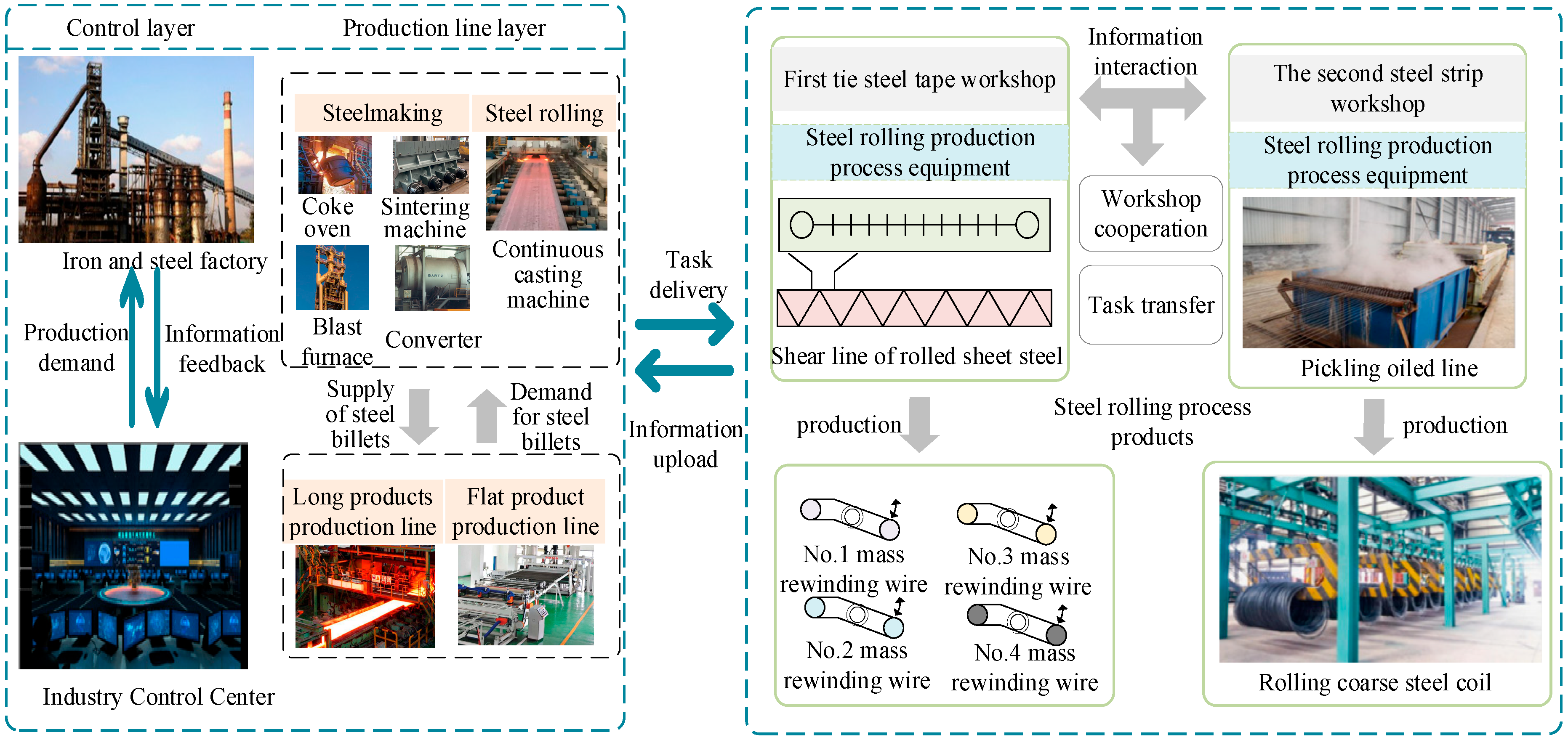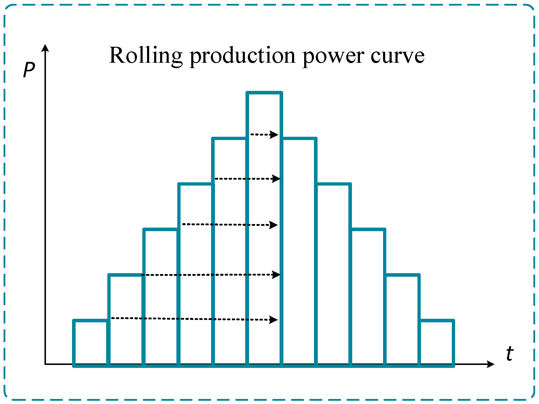Figure 1 and Figure 2 illustrate the power curve of a steel plant in a Chinese city, showing the rolling process. Steel billets first pass through roughing mills, followed by multi-pass rolling, before entering the finishing mills, where they move at a constant speed. Each pass through a mill induces power fluctuations due to mechanical impacts on the billets.

Taking the production of medium-thick steel plates as an example, the power required for the rolling process of billet steel can be expressed as follows:

$$P_n\left(t\right)=P_o^S\left(t\right)+P_o^E\left(t\right)+\sum _{i=1}^n\sum _{j=1}^m\left(P_i^S\left(T_j\right)+P_i^E\left(T_j^{*}\right)\right)$$

(1)

where $P_n\left(t\right)$ represents total power; $P_o^S\left(t\right)$ and $P_o^E\left(t\right)$ represent the initial power of roughing train and finishing train, respectively; $P_i^S\left(T_j\right)$ and $P_i^E\left(T_j^{*}\right)$ respectively represent the i-th billet consumes T_j and $T_j^{*}$ hours of power in the j device in the roughing mill and the finishing mill.

Electric-arc furnace (EAF) refining technology utilizes electric-arc heating, argon stirring, and slag refining processes. Steel produced in the blast furnace is transferred to the refining furnace for further purification, where impurities are removed and alloy elements are added. The refined steel is then cast into various shapes in the continuous caster. During production, the refining furnace consumes significant amounts of electricity, with its power demand and operational rhythm demonstrating a certain level of flexibility. The furnace operates in batch mode, and its power can be adjusted by modifying the load tap changer settings. Traditional EAF production processes exhibit high-frequency harmonic components, creating a characteristic ‘striped’ fluctuation pattern. Upon completion of the refining process, the operator slowly raises the electrode to extinguish the arc, followed by cutting the power supply. The entire shutdown process is typically completed in seconds. With advancements in manufacturing technologies, low-carbon emission techniques, such as bottom tapping, are gradually being adopted in China.

EAF power is as follows:

$$P_{\mathrm{EA}}(t)=\left\{\begin{array}{cc}0& t⩽t_{\mathrm{on}}\\ {\displaystyle \frac{P_{e_i}}{t_s-t_{on}}}(t-t_{\mathrm{on}})& t_{\mathrm{on}}⩽t⩽t_s\\ (1+\alpha )P_{e_i}& t_s⩽t⩽t_x\\ {\displaystyle \frac{P_{e_i}}{t_{off}-t_x}}(t_{\mathrm{off}}-t)& t_x⩽t⩽t_{\mathrm{off}}\\ 0& t_{\mathrm{off}}⩽t\end{array}\right.$$

(2)

where $P_{\mathrm{EA}}(t)$ represents the operating power of electric-arc furnace at time t; t_on represents the time when the electric-arc furnace starts to power up and produce an arc; t_s represents the time from the start of the arc to reach a stable rated power; t_x represents the time required from the time when the operator issues the shutdown command to the time when the EAF power drops to 0; t_off represents the moment the electric arc furnace completely loses power; $P_{e_i}$ represents rated power of electric-arc furnace in normal operation; and $\alpha$ represents the random power fluctuation of electric-arc furnace under stable operation; it is usually set at 5% to 20% of the rated power.

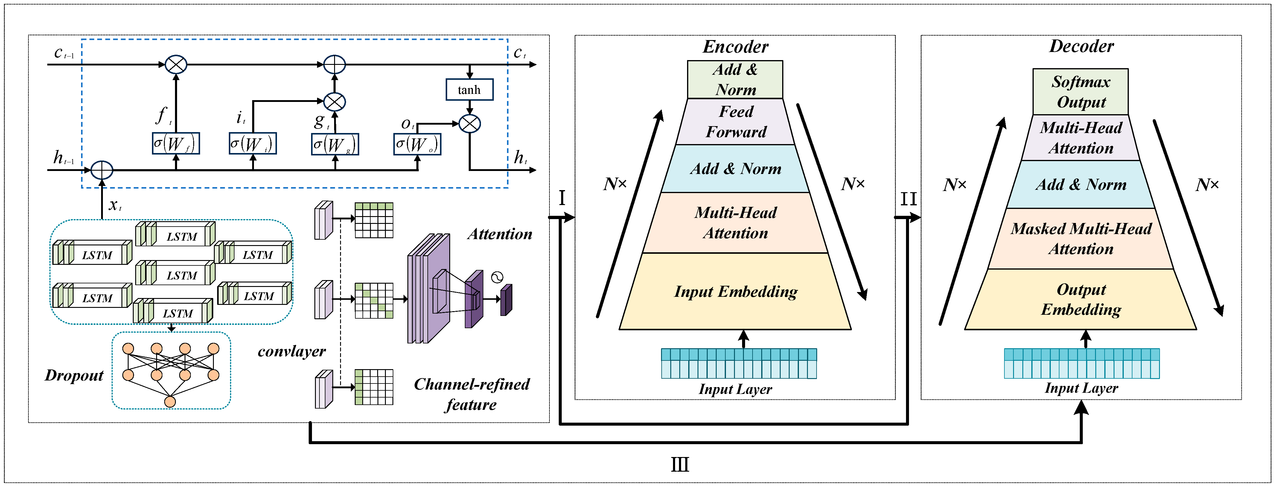
In addition to production loads, office and service departments in steel plants also contribute to electricity demand. These loads are mainly affected by working schedules and typically remain stable, as they are less influenced by production maintenance. When their share in the total consumption is small, they can be regarded as stable background loads. Due to the differences in volatility and seasonality between steel and air conditioning loads, a parallel Transformer-LSTM framework is applied for joint prediction. Steel loads are primarily related to production orders and exhibit relatively stable patterns, although cooling systems within plants show weather-related fluctuations. In contrast, air conditioning loads are strongly weather-driven and highly volatile. By incorporating these heterogeneous features into the joint prediction model, complementary adjustments are achieved without sacrificing accuracy. The Transformer captures global temporal dependencies, while the LSTM focuses on local variations, allowing the model to balance the distinct characteristics of both loads [27,28].

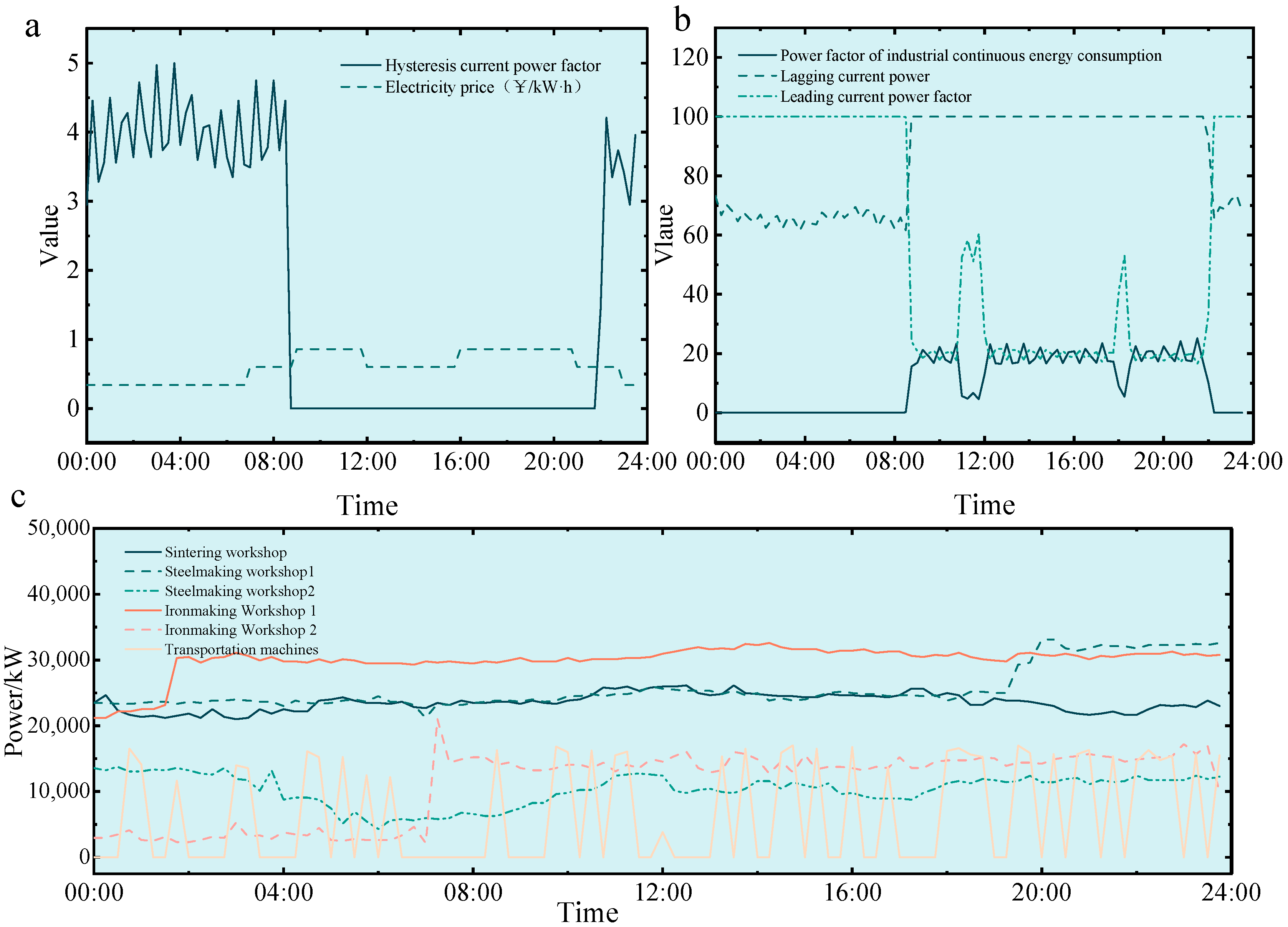
Figure 3 illustrates the hysteresis current power of steel loads, industrial continuous power consumption, lagging current factors, industrial electricity prices, and typical load curves for different workshops. The figure highlights the heterogeneity of load behaviors, showing both stable base consumption and fluctuating components driven by production and environmental conditions.

2.2. Physical Aggregation Model of Air Conditioner Equivalent Thermal Parameter (ETP)

The fluctuation of air conditioning loads is mainly influenced by weather conditions, whereas steel loads are closely related to production orders and equipment operating states. In this study, a joint prediction framework is proposed by combining the different characteristics of steel and air conditioning loads. Steel loads are generally stable during daily production; however, subsystems such as cooling units are also affected by ambient temperature, and their variations are therefore included as input features. In contrast, air conditioning loads exhibit significant seasonal fluctuations, especially during summer and winter peaks. The complementary nature of these two load types enables their joint prediction, where both fluctuation patterns are leveraged to improve overall forecasting accuracy and to support optimized grid scheduling strategies.

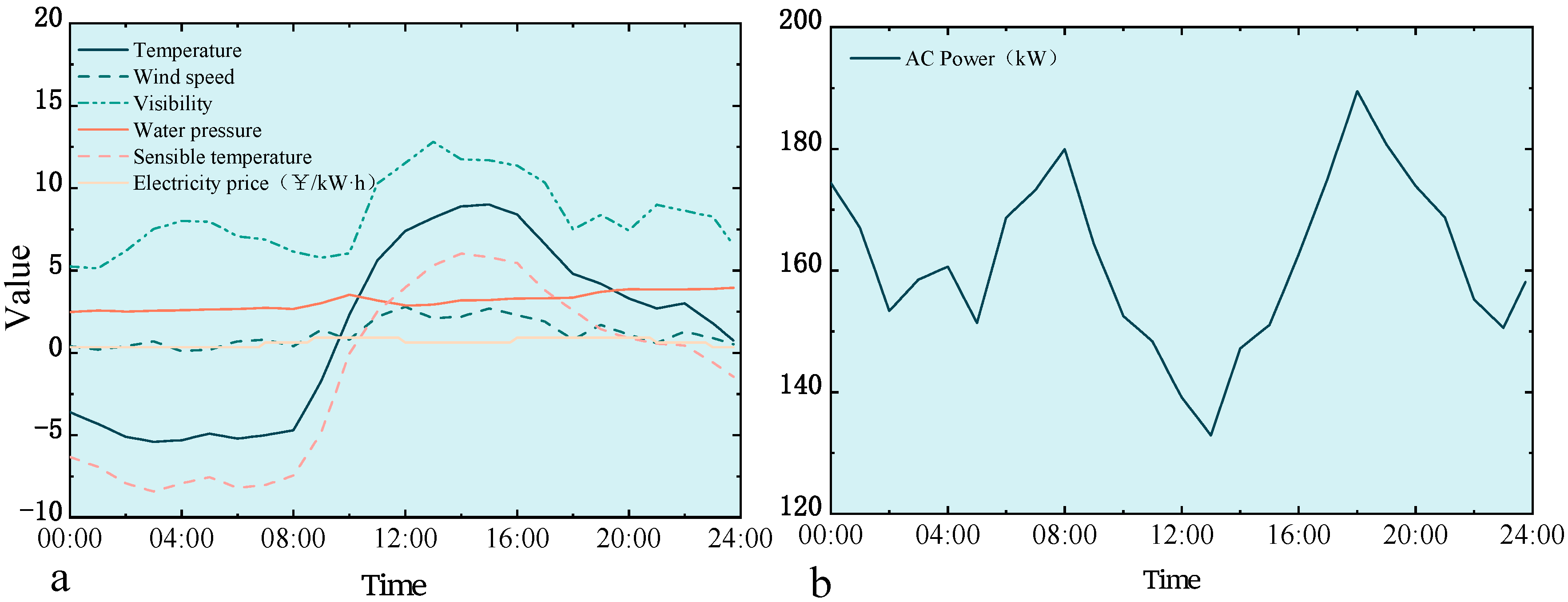
Figure 4 shows the input variables for air conditioning loads and their meteorological factors: (a) characteristics of weather influence and (b) typical load patterns.

Air conditioning load accounts for the largest share of electricity consumption in urban residential areas and possesses significant demand response potential. By constructing its thermodynamic equivalent model, the operational status of a single air conditioner can be simulated. The thermodynamic model of a single air conditioner is formulated as follows:

$$P^{LAC}={\displaystyle \frac{-\frac{d{T}_{in}(t)}{dt}c\cdot R_o-T_{in}(t)+T_{out}(t)}{\gamma (t)R_o}}$$

(3)

where $T_{in}(t)$ and $T_{out}(t)$ represent the real time temperature indoor and outdoor temperature, respectively; $c$ represents the equivalent heat capacity; $R_o$ represents the total thermal resistance; $P^{LAC}$ represents the cooling power of residential air conditioners; $\gamma (t)$ represents the switching time of the air conditioner; and 1 and 0 represent the air conditioner power, on and off, respectively.

Based on the switching time of the air conditioner, its operational behavior can be determined by solving the first-order linear differential equation in Equation (4):

$$\left\{\begin{array}{l}{{\displaystyle e}}^{{\displaystyle \frac{T^{\mathrm{on}}}{c{R}_o}}}={\displaystyle \frac{P^{\mathrm{LAC}}{R}_o+T^{\mathrm{set}}+\tau /2-T^{out}}{P^{\mathrm{LAC}}{R}_o+T^{\mathrm{set}}-\tau /2-T^{out}}}\\ {{\displaystyle e}}^{{\displaystyle \frac{T^{\mathrm{off}}}{c{R}_o}}}={\displaystyle \frac{T^{out}-T^{\mathrm{set}}+\tau /2}{T^{out}-T^{\mathrm{set}}-\tau /2}}\end{array}\right.$$

(4)

where $T^{\mathrm{set}}$ represents the set temperature for the air conditioner, $\tau$ represents the temperature dead zone; and $T^{\mathrm{on}}$ and $T^{\mathrm{off}}$ represent the air conditioning on and off time, respectively.

In the same distribution area, the load characteristics of all air conditioners are similar, so their equivalent thermal capacity, thermal resistance, and other parameters can be considered uniform. Following the method in [29], the aggregated load of the air conditioners can be expressed as:

$$P_{ag}(t)=\overline{N}Mp(t){\displaystyle \sum }_{\theta =16}^{31}X(t)L_{\theta }$$

(5)

where $P_{ag}(t)$ represents the aggregate power of the air conditioner at time t; $\overline{N}$ represents the average number of air conditioners per 100 households in the Taiwan district; M represents the number of residents in the Taiwan area; $p(t)$ represents the probability of the user turning on the air conditioner at time t; $X(t)$ represents the number of air conditioners at the temperature of $\theta$ at time t; and $L_{\theta }$ represents the air conditioning power at the temperature of $\theta$ at time t.

The startup rate and the probability of temperature set-points are determined from statistical data. The startup rate is estimated based on historical data from the same month of the previous year under similar weather conditions.

In addition, the linear relationship between air-conditioning load and temperature difference (ΔT) is analyzed using more than 30,000 samples collected from a region in China. As shown in Figure 5, the blue dots represent individual observations of air-conditioning load corresponding to different temperature differences. The data points are generally concentrated along the red regression line, indicating a strong and significant positive correlation between the two variables. The residual plot on the right further illustrates that the residuals (blue dots) are randomly scattered around the zero line, with no apparent pattern or systematic bias. This random distribution suggests that the model’s linearity assumption is valid and that the regression adequately captures the main relationship between air-conditioning load and ΔT.

3. Parallel Transformer-LSTM Model for Load Prediction

3.1. Parallelized Transformer-LSTM Model for Load Prediction

The Transformer architecture primarily consists of position encoding, a multi-head attention mechanism, and a feed-forward neural network. To better capture positional information in long-sequence processing, position encoding is applied. The fundamental equation is as follows:

$$\left\{\begin{array}{l}{W}_{\mathrm{E}(q,2i)}=\sin (q/{10000}^{2i/d})\\ W_{\mathrm{E}(p,2i+1)}=\cos (q/{10000}^{2i/d})\end{array}\right.$$

(6)

where $q$ represents position in the time series; $i$ represents the index of the feature dimension; $d$ represents the embedded dimension of node load; and $k$ represents a natural number.

The input to the self-attention network requires position encoding:

$${\mathit{E}}_t[i,:]={\mathit{e}}_t[i,:]+\mathit{p}$$

(7)

where $\mathit{p}$ represents the positional encoding of fusion parity dimensions; ${\mathit{e}}_t$ represents the load information matrix of a single node; and ${\mathit{E}}_t$ represents the self-attention level total input.

The multi-head self-attention mechanism in the Transformer processes multiple attention heads in parallel, enabling the model to capture diverse contextual features within the input representations.

$$\left\{\begin{array}{l}{H}_{\mathrm{att}i}=\mathrm{softmax}({\displaystyle \frac{Q{K}^{\mathrm{T}}}{\sqrt{d}}})V\\ H_{\mathrm{matt}}=W_{\mathrm{matt}}[H_{\mathrm{att}1},H_{\mathrm{att}2},...,H_{\mathrm{att}h}]\end{array}\right.$$

(8)

where $d$ represents the dimensional size of the model; $H_{\mathrm{att}}$ represents the attention value of load correlation; $Q$ and $K$ represent the query vector and key vector, respectively; and $V$ represents load history data eigenvalue vector.

To optimize the performance of the Transformer and enhance its ability to capture local features, a parallel approach using both the Transformer and LSTM is employed. By using two branches for parallel learning, the model is able to extract and process information across different time scales: the Transformer handles global temporal features, effectively capturing long-term behavioral patterns in sequential data, while the LSTM processes local temporal features, enabling it to capture short-term dynamics and changes in the data sequence. This architecture is illustrated in Figure 6.

3.2. Quantile Regression Interval Evaluation

During the steel production process, load fluctuations can occur rapidly, with power variations reaching hundreds of megawatts. Similarly, the start-stop behavior of large-scale air conditioning loads in the substation area may cause significant deviations between the model’s estimated and actual values. To address this, this paper introduces the Quantile Regression (QR) method, which considers the probabilistic distribution characteristics of the sample data. QR calculates the regression results of the dependent variable relative to the independent variables at different quantiles, providing the functional relationship between them at a specific quantile. When a specific quantile is given, the QR method can estimate the predicted value at that quantile.

Assuming the error term follows a normal distribution, the QR method is applied to obtain the values of the dependent variable at the 0.05 and 0.95 quantiles, which represent the 90% confidence interval. The quantile regression model is defined as follows:

$$Q_Y(\tau |X)=\delta (\tau )X$$

(9)

where $Q_Y(\tau |X)$ represents the conditional quantile given by $Y$ at X = {x^t_i; i = 1, 2, …, n}; $\delta (\tau )$ = {$\delta {(\tau )}_i$; i = 1, 2, …, n} represents the parameter vector; and $\tau$ represents the quantile.

The parameter vector in Equation (10) can be determined by transforming the problem into a least-squares optimization formulation.

$$\underset{\delta (\tau )}{\min }\sum _{i\left|Y_i\ge \delta (\tau )X_i\right|}\tau {\left(Y_i-\delta (\tau )X_i\right)}^2+\sum _{i\left|Y_i<\delta (\tau )X_i\right|}(1-\tau ){(Y_i-\delta (\tau )X_i)}^2$$

(10)

where $i$ represents the serial number index of the sample; and $N$ represents the sample count.

3.3. CEEMDAN-VMD Steel-Load Data Noise Reduction Method

Steel-load data exhibit impulsive characteristics, necessitating an initial decomposition step to extract components at various frequencies. The CEEMDAN (Complete Ensemble Empirical Mode Decomposition with Adaptive Noise) method enhances traditional Empirical Mode Decomposition (EMD) and Ensemble EMD by incorporating adaptive Gaussian white noise. This technique decomposes the load data series into multiple Intrinsic Mode Functions (IMFs), with each IMF corresponding to a distinct level of fluctuation, based on frequency differences. The decomposition process is as follows:

Gaussian white noise is added to the signal x(t), followed by the application of the EMD method to process the mixed signal. The IMFs are separated from the signal after processing through EMD, isolating different frequency components.

$$E(x(t)+{(-1)}^q\partial x^j(t))=A_1^j(t)+z^j$$

(11)

In CEEMDAN decomposition, the sum of N modal components is calculated and averaged to obtain the first Intrinsic Mode Function (IMF). The first IMF is then subtracted from the original signal to yield the residual signal:

$$I(t)=x(t)-{\displaystyle \frac{1}{N}}\sum _{j=1}^N{A}_1^j(t)$$

(12)

A new signal is generated by adding paired positive and negative Gaussian white noise-to-signal $I(t)$. EMD is then applied to this new signal, with the first-order modal component $A_1^j(t)$ directly used as the second IMF in the CEEMDAN method. This process is repeated until the residual signal becomes monotonic, yielding $k$ IMF components. The original signal $y(t)$ is decomposed into multiple independent components:

$$x(t)=\sum _{k=1}^K\overline{A_k(t)}+I_i(t)$$

(13)

Subsequently, a variational framework is established using VMD to ensure the effective extraction of IMF. The Hilbert transform is applied to each mode function ${\stackrel{\wedge }{\mathrm{q}}}_i(\omega )$ to adjust the mode’s frequency to its respective reference frequency band. By solving the variational problem outlined in Equations (14)–(16), Lagrange multipliers $\lambda$ and penalty factor $\mathrm{\Omega }$ are introduced, and the solution to the quadratic optimization problem is derived iteratively.

$${\stackrel{\wedge }{\mathrm{q}}}_k^{n+1}(\omega )={\displaystyle \frac{\stackrel{\wedge }{\mathrm{f}}(\omega )-\sum ^{\wedge }{\stackrel{\wedge }{\mathrm{q}}}_i(\omega )+\frac{\stackrel{\wedge }{\lambda }(\omega )}{2}}{1+2\mathrm{\Omega }{\left(\omega -{\omega }_k\right)}^2}}$$

(14)

$${\omega }_k^{n+1}={\displaystyle \frac{{\int }_0^{\infty }\omega |\stackrel{\wedge }{q}(\omega ){|}^{2}d\omega }{{\int }_0^{\infty }|q(\omega ){|}^{2}d\omega }}$$

(15)

$${\stackrel{\wedge }{\lambda }}^{n+1}={\stackrel{\wedge }{\lambda }}^n+\tau (\stackrel{\wedge }{f}-{\displaystyle \sum {\stackrel{\wedge }{\mathrm{q}}}^{n+1}})$$

(16)

4. Coordinated Optimization Scheduling Strategy for Steel-Industry- and Air Conditioning-Load Clusters

In the steel manufacturing industry, processes such as the operation of the electric-arc furnace (EAF) are based on electrical heating principles. The inherent thermal inertia of electric heating loads means that even in emergency situations, the temperature of the EAF does not immediately decrease significantly after the arc is quickly shut down. Additionally, a buffer inventory area exists between the EAF stage and subsequent processes in the steelmaking flow, allowing for a 0.5-min startup delay without disrupting the overall production process. Due to the interruptibility and dispatchability of the EAF, it can be leveraged as a tool for demand-side management. In emergency situations, strategically pausing or delaying the startup of equipment within this area can effectively mitigate power fluctuations in the steel plant. By adjusting the EAF, roughing mill, and finishing mill equipment, a maximum load reduction can be achieved during the operation period, as calculated by the following formula:

$$\mathsf{\Delta }\mathrm{P}=(v_1{P}_S+v_2{P}_E+v_3{P}_{EA})\tilde{\tau }$$

(17)

where $v_1$, $v_2$, and $v_3$ represent, respectively, the maximum power regulation ratio of the roughing mill, the finishing mill, and the electric-arc furnace to minimize the impact on production; $P_S$ and $P_E$ represent, respectively, the current running power of roughing mill and finishing mill; $\mathsf{\Delta }\mathrm{P}$ represents the total load that can be reduced, and $\tilde{\tau }$ represents the duration of the cuts.

When an air conditioner operates under steady-state conditions, its power consumption exhibits a linear relationship with the indoor–outdoor temperature difference. Assuming the outdoor temperature remains constant over the short term, the power consumption of the air conditioner also shows a linear dependence on the set temperature. Prior to demand response activation, the compressor operates intermittently to maintain the indoor temperature near the set point. Upon initiating demand response, users follow load adjustment instructions (LA) to raise the set temperature, thereby entering the dynamic adjustment phase. During this phase, the compressor stops, and the indoor temperature gradually increases until it reaches the new set point, at which point the compressor restarts and resumes intermittent operation, transitioning into a static phase. Under identical outdoor conditions, an increase in the set temperature significantly reduces the total power consumption, thus enhancing the scheduling potential.

The aggregated power when the set temperature is 23 °C is defined as the baseline value, P_r, and after adjusting the set temperature, the new aggregated power is P_n. The regulatory potential P is the difference between these two values. The proposed cooperative optimization scheduling strategy for steel plants and air conditioning load groups calculates the aggregated air conditioning power in the substation area based on Equation (5). It determines the optimal adjustment of the set temperature to uncover the adjustable potential of the temperature control load group without affecting user comfort. LA instructions are then used to mitigate the power impact from steel plant loads. Finally, an optimal scheduling scheme is determined through various electric arc furnace start-stop strategies, coordinating steel and air conditioning loads to stagger peak usage times, avoid exacerbating power supply and demand conflicts, and achieve peak shaving and valley filling by reducing air conditioning power consumption during peak periods while ensuring resident comfort. The coordination strategy process between steel and air conditioning is shown in Figure 7.

5. Simulation Results and Discussion

5.1. Research Scenario

To validate the accuracy of the proposed model, real measurement data from a steel plant in China were used for a simulation analysis. In 2023, the plant produced over 2 million tons of steel, with a total electricity demand of approximately 1025.273 MW. The plant consists of several workshops, including the intelligent ironmaking factory, sintering workshop (comprising large fans, oxygen machines, and wastewater treatment facilities), steelmaking workshops (including blast furnaces, and sintering machines), and rolling mills. Additionally, within the same district, 35,038 records of air conditioning loads were collected at 15-min intervals.

The uncertainty of the interval estimates was quantified by the interval mean width, with smaller widths indicating higher reliability. Model accuracy was further evaluated using multiple metrics, including mean square error (MSE), root mean square error (RMSE), mean absolute error (MAE), mean absolute percentage error (MAPE), and the coefficient of determination (R²). The parameter settings for CEEMDAN decomposition, Transformer encoder, and LSTM layers are summarized in

Table 1. Parameter settings.

Type	Optimized Parameter	Search Range	Selected Value
CEEMDAN Parameters	Noise weight	[0.1, 0.5]	0.2
	Number of noise additions	[100, 1000]	500
	Max iterations for envelope	[2000, 6000]	5000
Transformer Encoder Parameters	Embedding dimension	[64, 512]	256
	Number of attention heads	[4, 16]	8
LSTM Layer Parameters	Hidden units	[64, 256]	128
	Dropout rate	[0.1, 0.5]	0.3

, where the optimized values were selected within their respective search ranges.

5.2. Data Preprocessing

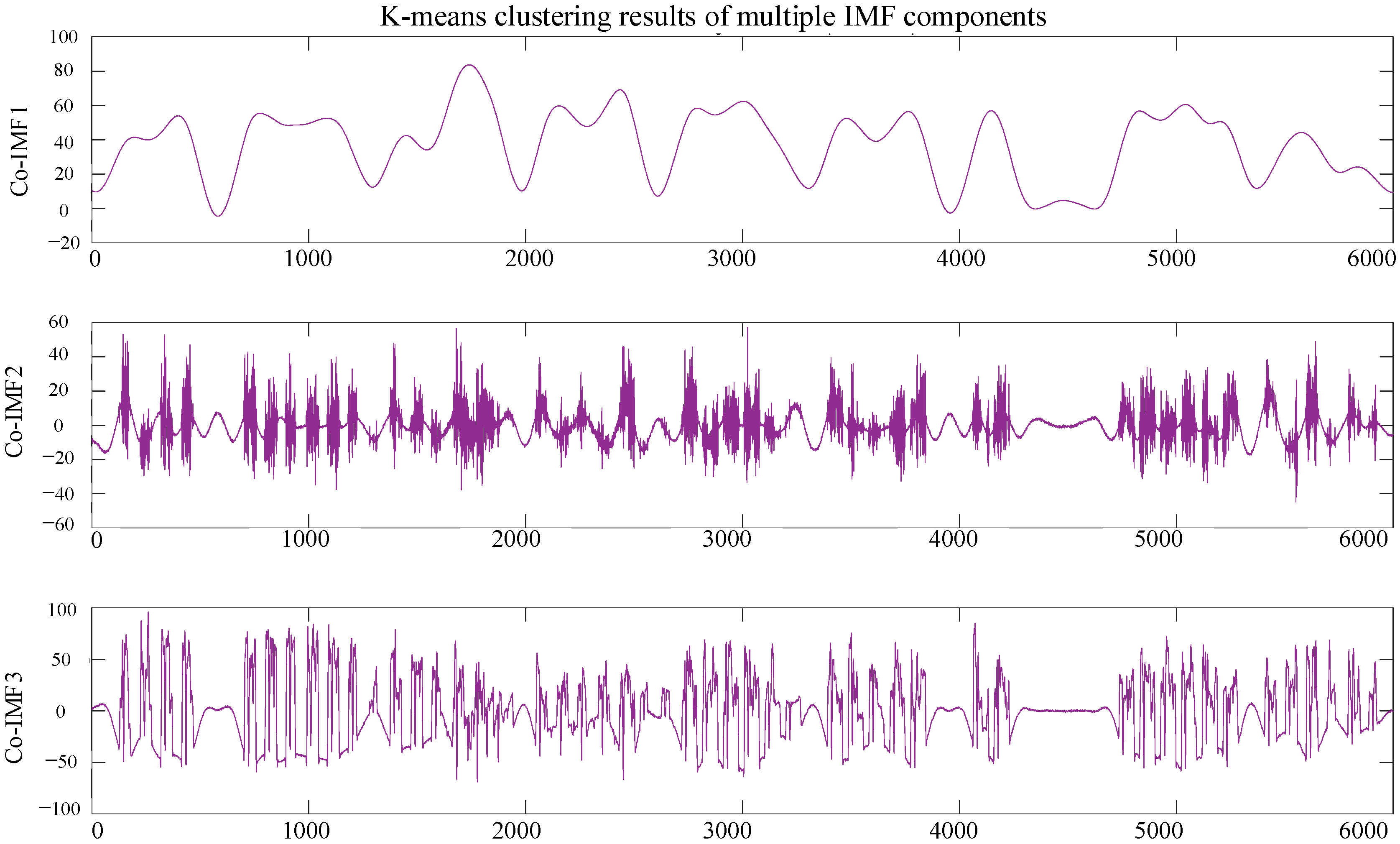
In this approach, load data from a steel plant, consisting of 35,041 data points, was first preprocessed and decomposed using the CEEMDAN-VMD method. This decomposition process separated the data into distinct frequency components, where high-frequency components captured abrupt fluctuations, while low-frequency components reflected long-term trends. The decomposition was performed using a noise weight of 0.2, 500 noise realizations, and a maximum envelope count of 5000. As a result, the CEEMDAN-VMD method generated 14 components, which were categorized into three groups: (1) high-frequency components (IMF1 to IMF7), characterized by frequent and irregular fluctuations; (2) low-frequency components (IMF8 to IMF13), exhibiting smoother long-term variations; and (3) the trend component (IMF14), which captured the overall load evolution, as shown in Figure 8.

As shown in Figure 8 and Figure 9. To quantify the complexity of the components, sample entropy was calculated, followed by k-means clustering to classify them based on entropy values. The high-frequency component, Co-IMF1, was further decomposed using Variational Mode Decomposition (VMD) into finer frequency components, Co-IMF2 and Co-IMF3. These components served as target outputs for a neural network model, which was trained to predict each component separately. The predicted components were then aggregated to reconstruct the final load prediction for the steel plant.

This approach integrates decomposition techniques and neural networks to enhance prediction accuracy by systematically analyzing data across multiple frequency levels.

The selection of input variables has a significant impact on the predictive performance of the model. In this study, Spearman’s correlation coefficient was used to evaluate the relationships between steel and air conditioning loads, production rhythm, and weather information. Variables with higher absolute correlation values were retained as key influencing factors for joint prediction. The steel plant load data mainly included electric arc furnaces (EAFs), rolling mills, and auxiliary systems. To ensure consistency with air conditioning loads, the sampling interval was uniformly set to 15 min, producing 96 data points per day. Missing values were filled using a sliding window moving average, which smoothed fluctuations and reduced errors in subsequent analysis. Outliers were identified by the 3σ criterion; random errors were removed, while abnormal values related to actual production events were corrected with adjacent averages. The processed dataset and results are presented in Figure 10.

As illustrated in Figure 11, correlation coefficients for both air conditioning and steel loads were computed. Weather and industrial process variables with absolute correlation coefficients exceeding 0.3 were selected as input features to enhance the model training efficiency. Key influencing factors for air conditioning loads include outdoor temperature, perceived temperature, water vapor pressure, and electricity prices. For steel loads, significant factors include industrial continuous energy consumption, carbon dioxide concentration (ppm), lagging current power factor, and industrial electricity prices. These variables were incorporated as primary predictors in the steel–air conditioning load forecasting model.

The detailed results of the correlation analysis are presented in

Table 2. Correlation of factors influencing AC load.

Influencing Factors	Humidity	Temperature	Wind	Pressure	Precipitation	Visibility	Water Pressure	AT	Price
Spearman coefficient	0.10	0.33	0.05	−0.24	0.00	0.05	0.35	0.34	0.29

and

Table 3. Correlation of factors influencing steel load.

Influencing Factors	Lagging Current Reactive	Leading Current Reactive	CO2	Lagging Current Power	Leading Current Power	NSM	Price
Spearman coefficient	0.64	−0.13	0.88	0.38	0.19	0.32	0.56

. Table 2 shows that outdoor temperature (0.33), perceived temperature (0.34), and water vapor pressure (0.35) exhibit relatively strong correlations with air conditioning loads. Table 3 indicates that CO₂ concentration (0.88), lagging current reactive power (0.64), and electricity prices (0.56) are the dominant factors for steel loads. These findings confirm the appropriateness of the selected features for subsequent model development.

5.3. Forecasting Outcomes for Steel and Air Conditioning Load Groups

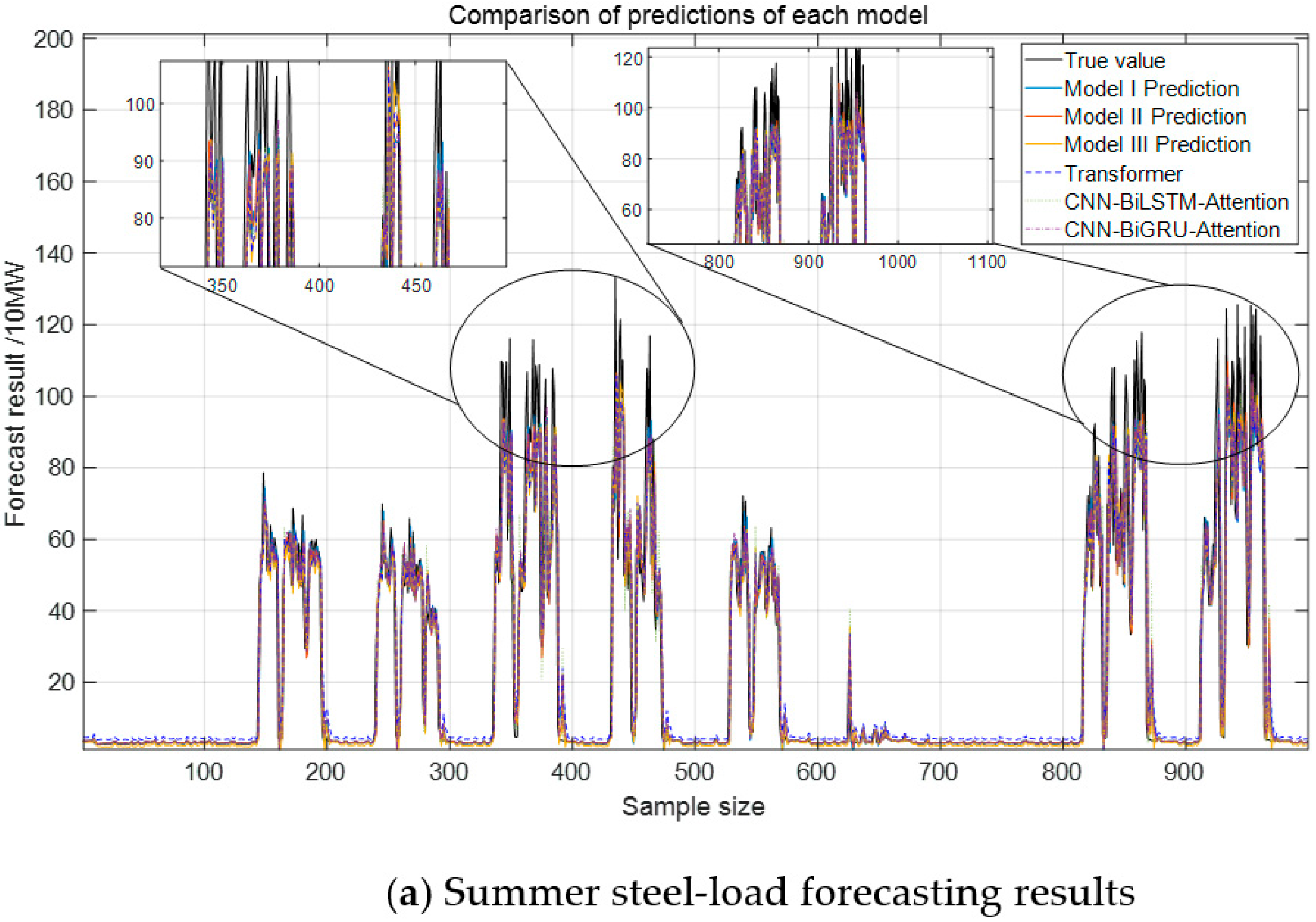
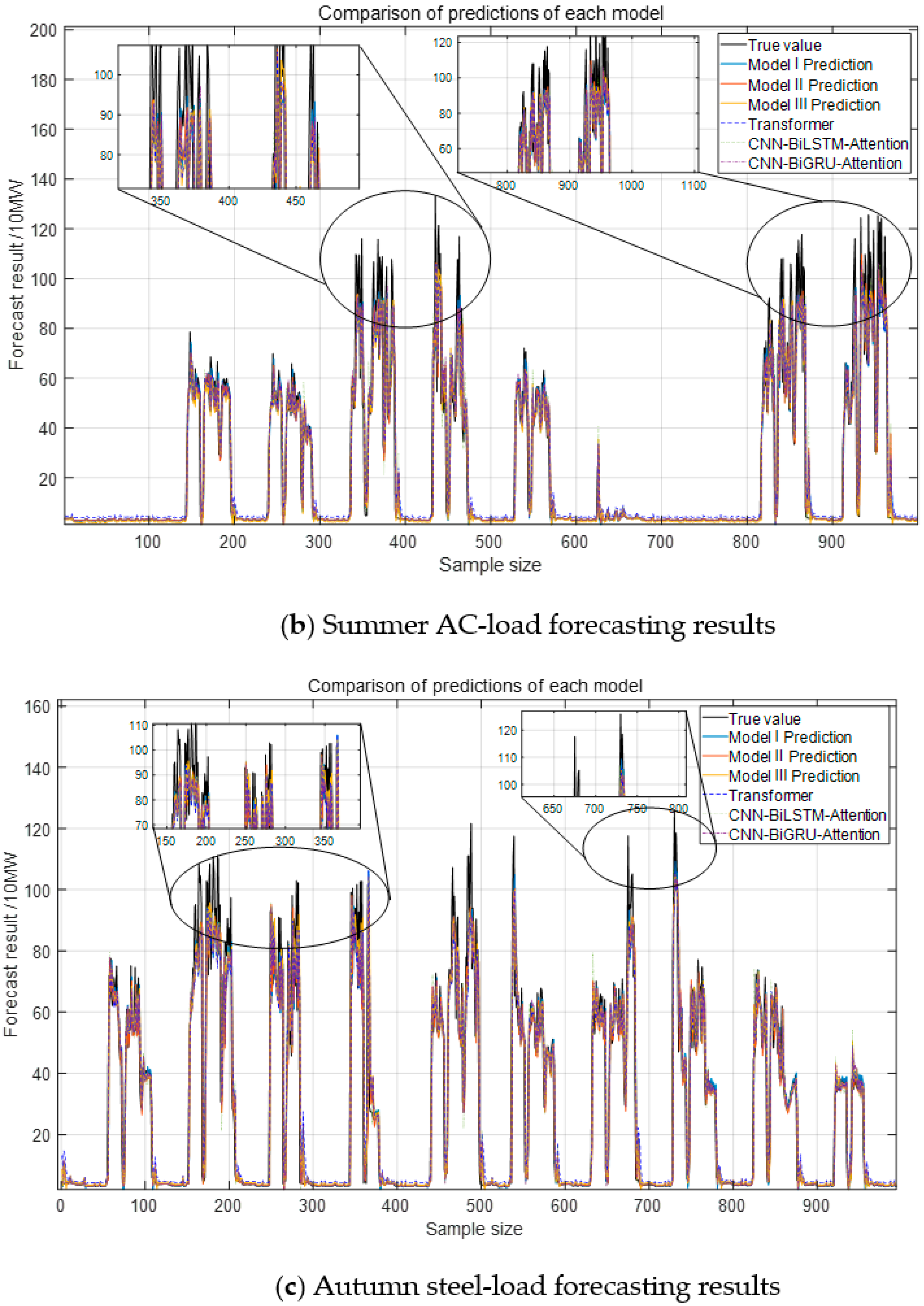
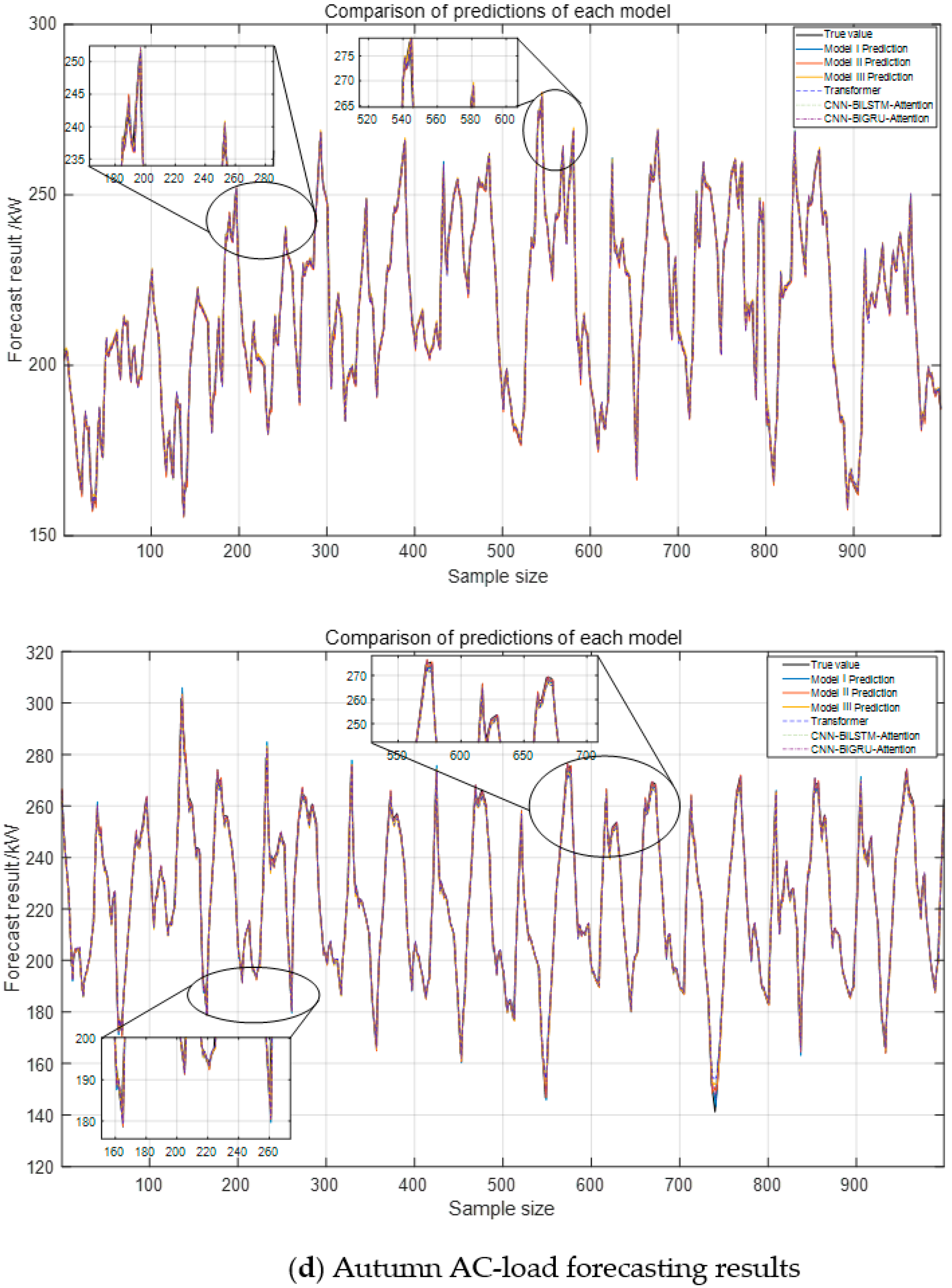
To compare the predictive accuracy between raw and CEEMDAN-VMD decomposed data, we adopted a training-to-test ratio of 8:2 and selected a state-of-the-art bi-directional neural network model for benchmarking, as referenced in [30,31,32,33]. The results, presented in Figure 11, indicate that the proposed Model III model closely aligns with the actual load curve. In contrast, other models, constrained by convolutional operations, primarily capture local features while failing to extract critical information from the original data and external factors, leading to reduced accuracy.

To ensure model robustness and avoid data leakage, we implemented a rolling-backtest approach with dynamic moving training/validation windows. Initially, we tested with a training-to-validation ratio of 7:3 and 6:4, but after evaluating performance across different conditions, we found that an 8:2 split provided the best balance between training efficiency and accuracy. During the rolling-backtest, each time the model was validated, only data from the training window (prior to the “origin” time) were used for validation, ensuring no future data were leaked into the model. This approach prevents overfitting and time-dependent bias, offering a more realistic performance evaluation.

To further assess the model’s generalizability across varying climate conditions, we conducted tests during peak air conditioning periods in summer and autumn, when fluctuations in humidity, temperature, and steel plant scheduling are significant.

From the analysis of Figure 12, the proposed Model III model demonstrates the best performance across evaluation metrics, reducing the error by approximately 2.32% compared to the CEEMDAN-VMD decomposition method. This improvement is attributed to the incorporation of adaptive Gaussian white noise in the decomposition process. The model achieves 150% higher predictive accuracy for steel load compared to air conditioning load due to the latter’s stability and strong correlation with weather factors. In contrast, the steel load is influenced by factory process rhythms and frequent load shocks, introducing greater variability and reducing prediction accuracy.

Model I adopts a sequential Transformer-LSTM structure, where the Transformer first extracts global temporal dependencies, followed by LSTM capturing short-term fluctuations. Model II reverses this sequence, applying LSTM before Transformer to refine local features before global context processing. While both models leverage bidirectional information, they remain constrained by sequential computations, lacking the parallel structure of Model III.

From

Table 4. Training performance comparison of joint prediction models with different methods in summer (steel/AC, * represents the algorithm in this paper).

Method	MSE	RMSE	MAE	MAPE/%	R2/%
Model Ⅰ	160.00/7.99	12.65/2.83	5.79/1.77	28.74/0.80	83.87/99.01
Model Ⅱ	155.31/7.99	12.46/2.83	5.58/1.85	26.27/0.85	84.35/99.01
Model Ⅲ *	154.12/7.06	11.45/2.66	5.38/1.53	25.45/0.69	83.36/99.13
Transformer	157.60/8.52	12.55/2.92	5.84/2.01	33.78/0.89	84.13/98.95
CNN-BiLSTM- Attention	160.78/8.94	12.68/2.99	6.52/2.05	53.38/0.93	83.79/98.89
CNN-BiGRU- Attention	158.49/8.65	12.59/2.94	5.58/1.92	26.03/0.88	84.03/98.93

and

Table 5. Training performance comparison of joint prediction models with different methods in autumn (steel/AC). (* represents the algorithm in this paper).

Method	MSE	RMSE	MAE	MAPE/%	R2/%
Model Ⅰ	151.84/7.39	12.32/2.72	6.17/1.61	30.09/0.75	84.82/98.88
Model Ⅱ	149.48/7.03	12.22/2.65	6.02/1.53	27.63/0.70	85.06/98.94
Model Ⅲ *	140.06/6.59	11.83/2.57	5.78/1.51	26.34/0.70	85.99/99.109
Transformer	148.66/7.14	12.19/2.67	6.24/1.63	34.92/0.77	85.14/98.92
CNN-BiLSTM- Attention	150.73/7.12	12.28/2.66	6.77/1.57	49.63/0.74	84.93/98.83
CNN-BiGRU- Attention	146.41/7.53	12.10/2.74	6.04/1.67	28.89/0.78	85.36/98.86

, it can be observed that Model III achieves more favorable results with respect to several metrics. In summer experiments, Model III reduces MAPE by 11.5% compared with Model I (28.74% → 25.45%) and by 24.7% compared with CNN-BiLSTM-Attention (33.78% → 25.45%), while maintaining an R² above 99% for AC loads. In autumn, Architecture III lowers MAPE by 12.4% compared with Model I (30.09% → 26.34%) and by nearly 47% compared with CNN-BiLSTM-Attention (49.63% → 26.34%). At the same time, the coefficient of determination (R²) reaches about 86% for steel loads, which is slightly higher than for Models I and II. These findings indicate that changing the order of Transformer and LSTM provides only marginal benefits, whereas the parallel combination in Model III yields more consistent improvements across different indicators. In addition, compared with point predictions, interval estimation offers a broader representation of fluctuations, which is valuable for capturing steel-load shocks and facilitating timely demand response [34].

5.4. Collaborative Demand Response Strategy for Steel and Air Conditioning Loads

This section investigates the air conditioning usage patterns of approximately 2000 households in a region of China, based on the fact that 145.9 air conditioners are owned per 100 urban households. As shown in Figure 13, panels (a) to (d) illustrate the relationships between user comfort level, demand response willingness, and air conditioning load shedding under the influence of user-set temperature preferences and air conditioning on/off rates. Additionally, the adjustable load potential is analyzed in relation to the impacts of air conditioning on/off rates and user temperature preferences. The residents in this region predominantly set their temperature preferences within the range of 18–30 °C. For comfort, the highest level is observed when the temperature is maintained at around 25 °C, and the air conditioning on/off rate is high. As the on/off rate decreases, the comfort level declines at a rate of approximately 5% per unit reduction in the on/off rate. Similarly, demand response willingness follows a trend similar to comfort, with the highest willingness occurring at the 25 °C setting, reaching a value of approximately 0.8. As the on/off rate decreases, the willingness decreases at a rate of approximately 1% per unit reduction in the on/off rate. In contrast, the degree of air conditioning load shedding is inversely proportional to the on/off rate; the higher the on/off rate, the lower the load shedding degree, with the highest shedding occurring at a temperature setting of 25 °C. Regarding the adjustable load potential, the optimal load regulation is achieved when the temperature is set to 24 °C and the air conditioning on/off rate is near 0%, where the load adjustment level reaches its peak while considering user comfort.

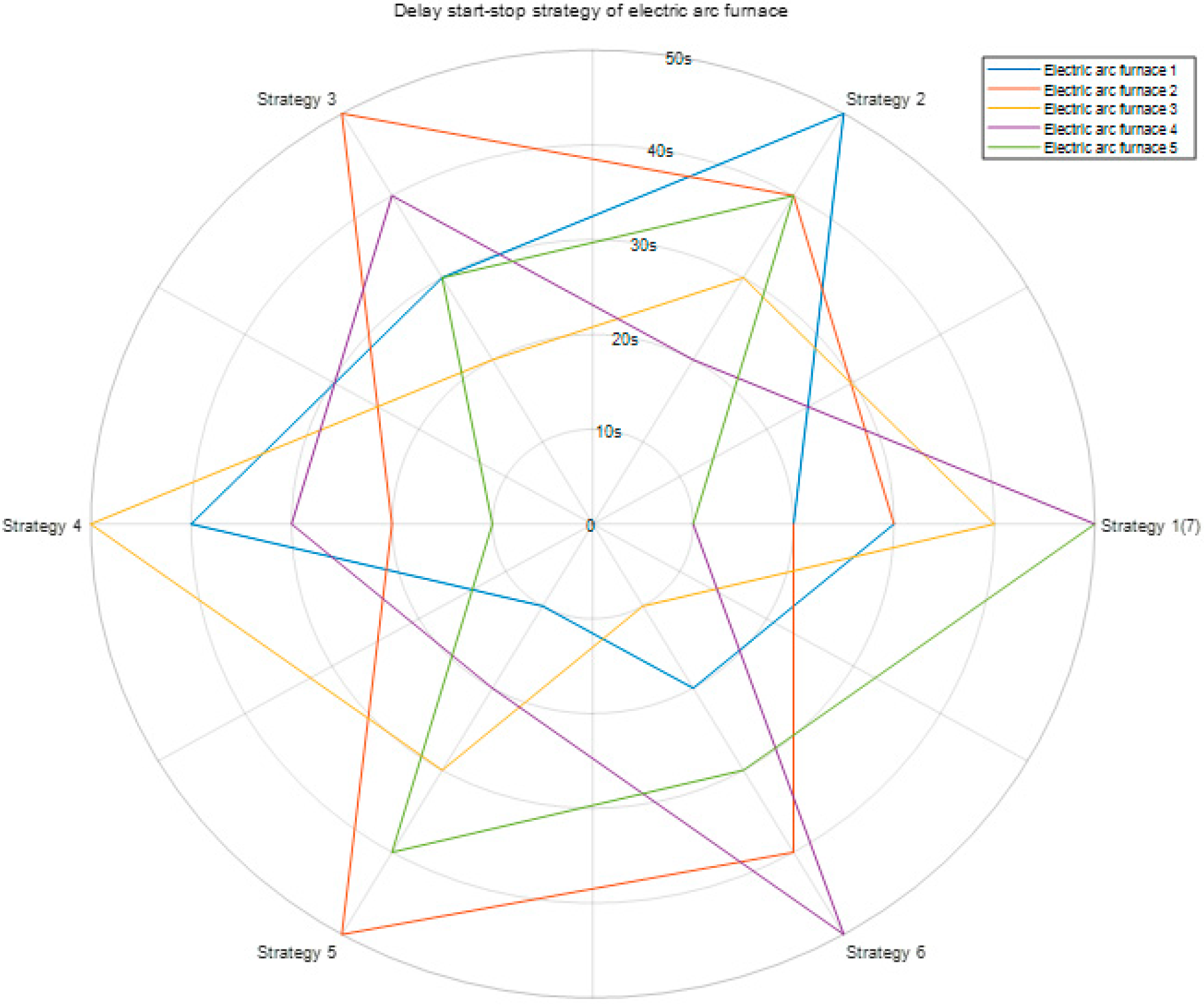
In the context of demand-side response, the load from electric-arc furnaces (EAFs) in steel enterprises can be optimally adjusted within a short time frame, allowing for flexible start-stop control without disrupting production schedules. This approach helps to mitigate the impact on the power grid. By precisely controlling the start-stop sequence of EAFs, power consumption can be optimized, thereby alleviating the burden on the power system. For this analysis, 600 load data points were collected over a given period, and the proposed model was applied to optimize the load sequencing. During this period, the steel plant included two rolling mills, five electric-arc furnaces, three continuous casting lines, and approximately 300 MW of other loads.

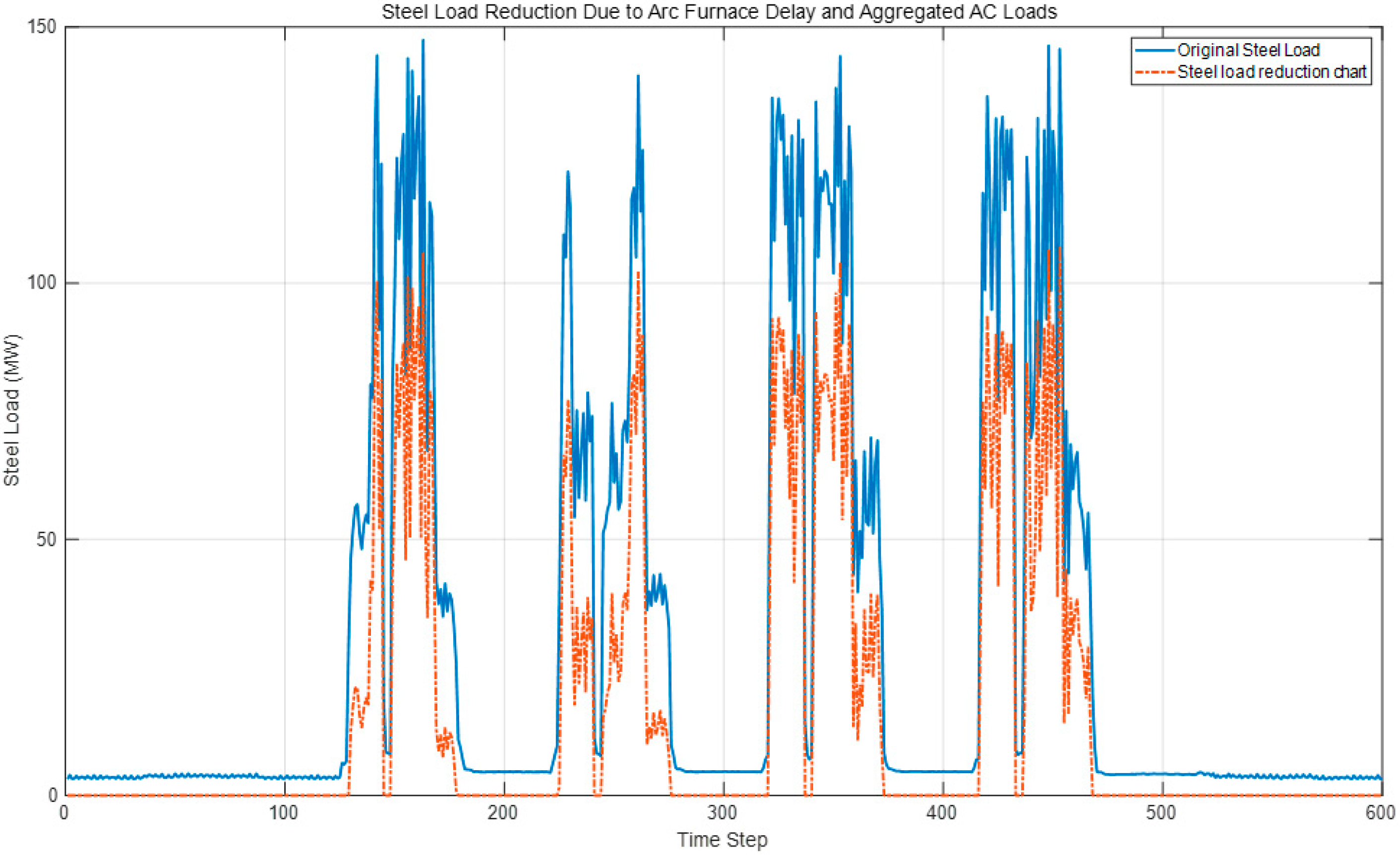
Based on the preliminary prediction, an optimization strategy for the startup and shutdown sequence of the five refining furnaces in the steel plant was proposed, comprising seven scenarios, as depicted in Figure 14. These strategies consider load balancing while integrating the potential for air conditioning load reduction. Figure 15 demonstrates the positive correlation between steel-load reduction and the compensatory effects of air conditioning load adjustments under the combined optimization of electric-arc furnace scheduling and air conditioning load control. Specifically, the peak shaving range and variance reduction for steel loads reached 20.47% and 49.23%, respectively, with a user response willingness rate of 51%. According to the forecast, the air conditioning group can provide up to 20 MW of compensation for steel-load adjustments, offering significant flexibility for grid load regulation.

6. Conclusions and Future Work

This study develops a joint prediction and coordinated scheduling framework for steel loads and air conditioning clusters. By integrating decomposition techniques with a parallel Transformer-LSTM structure, the model achieves higher forecasting accuracy compared with benchmark methods, with MAPE reductions of up to 24.7% in summer and 47% in autumn. When applied to coordinated scheduling, the strategy reduces peak demand by about 9.6% and lowers load variance by approximately 13.4%, demonstrating its effectiveness for alleviating grid stress and smoothing demand profiles. These results highlight the potential of cross-sectoral demand response to enhance flexibility in real-world power systems.

In practical terms, the proposed scheduling framework can be applied through advanced metering and control infrastructures, where residential air conditioning clusters respond rapidly to price signals while steel enterprises participate within operational safety limits. Such coordination contributes to demand-side management by balancing system efficiency with user constraints, reducing the need for costly grid reinforcements, and supporting renewable energy integration. Future work will extend the approach to additional industrial loads, refine incentive mechanisms, and validate the strategy through pilot projects under real communication and control environments.