Abstract
The flexible job shop scheduling problem (FJSP) becomes significantly more complex when real-world factors such as due dates, sequence-dependent setup times, and processing times are considered as multiple criteria. This study presents a hybrid scheduling approach that combines a genetic algorithm (GA) and variable neighborhood search (VNS), where several dispatching rules are used to create the initial population and improve exploration. The multiple objectives are to minimize makespan, total tardiness, and total setup time while improving overall production efficiency. To test the proposed approach, standard FJSP datasets were extended with due dates and setup times for two different environments. Due dates were generated using the Total Work Content (TWK) method. This study also introduces a dynamic scheduling framework that addresses dynamic events such as machine breakdowns and new job arrivals. A rescheduling strategy was developed to maintain optimal solutions in dynamic situations. Experimental results show that the proposed hybrid framework consistently performs better than other methods in static scheduling and maintains high performance under dynamic conditions. The proposed method achieved 6.5% and 2.59% improvement over the baseline GA in two different environments. The results confirm that the proposed strategies effectively address complex, multi-constraint scheduling problems relevant to Industry 4.0 and smart manufacturing environments.
1. Introduction
In the manufacturing process, scheduling plays a crucial role in optimizing the use of resources and time. It involves decision-making to assign resources to jobs so that tasks are completed according to a planned schedule [1]. The demand for effective scheduling has grown significantly due to increasing market pressures for flexibility and timely delivery of products. The flexible job shop scheduling problem (FJSP) is an extension of the job shop scheduling problem (JSSP) that offers more flexibility by allowing operations to be processed on any available machine [2]. The FJSP is one of the most difficult combinatorial optimization problems due to its large solution space and number of possible combinations for assigning jobs to machines while dealing with various constraints [3], which is why it is classified as a non-deterministic polynomial-time hard (NP-Hard) problem [4].
Over the last few years, many researchers have proposed priority dispatching rules (PDRs) for ranking jobs. These rules are easy to implement, have lower complexity, and have the capacity to produce effective results in less time [5]. Simple priority rules utilize only one criterion, which might be the due date parameters, processing time, arrival time, or number of operations. Blackstone et al. used the first-in–first-out (FIFO) priority rule to select the next job in front of the queue, which is easy to implement [6]. Oliver and Chandrasekharan introduced a rule based on slack time to select the job with the minimum slack time, which helped to reduce the total tardiness of jobs [7]. Shi et al. proposed a multi-population genetic algorithm with an ER 20 network to address FJSP, demonstrating significant performance improvement over the traditional GA [8]. Jayamohan and Rajendran proposed new dispatching rules for shop scheduling and compared them with the shortest processing time (SPT) and the earliest due date (EDD). The composite dispatching rule (CDR) combines two or more SPRs. Tay and Ho proposed composite dispatching rules with GA for solving a multi-objective FJSP with criteria like released time and due dates [9]. Ozturk et al. applied gene expression programming to extract priority rules for a dynamic multi-objective FJSP. Their approach considered criteria such as due dates and release time, achieving improvement in makespan, mean lateness, and flow time as compared to traditional methods like FIFO and SPT [10]. Cheung and Zhou proposed a hybrid algorithm integrating genetic algorithms and heuristic rules for solving the JSSP with sequence-dependent setup time [11]. Cemal et al. contribute to mixed integer programming models for the FJSP with separable and non-separable sequence-dependent setup times [12]. Dos Santos et al. used NSGA for multi-objective optimization while considering sequence-dependent setup times and machine-dependent setup times to schedule jobs on unrelated parallel machines, demonstrating the effectiveness of evolutionary approaches in minimizing makespan and average completion time [13]. Meguel et al. proposed an integrated dispatching algorithm using fuzzy AHP and TOPSIS for scheduling flexible job shop systems [14]. Thenarasu et al. combined discrete event simulation (DES) with decision-making methods, focusing on multi-criteria scheduling problems, considering factors like due dates and setup time, with objectives like minimizing makespan and tardiness [15]. Liu and Qin proposed an improved GA framework for the FJSP where the multiple objectives are maximizing makespan, balancing machine load, and resource utilization [16]. Gong et al. addressed the distributed FJSP with job priority using the new memetic algorithm with multiple objectives, such as reducing resource waste and time loss by unreasonable production plans [17]. Sels et al. performed detailed research evaluating various priority rules for the FSSP under multiple objectives. Their research evaluated both simple and hybrid priority rules, including dynamic job arrivals and sequence-dependent setup time [18]. Rahmati et al. developed a non-dominated ranking genetic algorithm (NRGA), with objectives such as makespan, critical machine workload, and total workload of machines [19]. Draz et al. proposed a hybrid metaheuristic framework that combines bio- and natural-inspired algorithms to improve scheduling and energy efficiency in an underwater Internet of Things network [20]. Tay and Ho applied the GA to evolve composite dispatching rules for the multi-objective FJSP, with objectives of makespan, mean tardiness, and mean flow time [21]. Willian et al. proposed a method that uses metaheuristics, including the GA and tabu search (TS), to solve the online printing shop scheduling problem with criteria sequence-dependent setup times and a single objective minimizing makespan [22]. The hybrid metaheuristic algorithm was proposed to address dynamic events like job arrivals in the FJSP [23]. The genetic algorithm (GA) with a hybrid approach was presented by Ben Ali et al. for addressing the new job arrival in the JSP to minimize the makespan [24]. Tariq et al. proposed a framework for dynamic scheduling, like machine breakdown, which addresses challenges in the FJSP in the manufacturing industry [25]. Said Gattoufi et al. propose an improved GA combined with local search to solve the DFJSP to minimize makespan [26]. Le Mai Thi et al. proposed an improved hybrid metaheuristic approach for solving dynamic events such as machine breakdowns, with objectives including minimizing makespan and improving stability. The approach integrates the GA with heuristic rules to efficiently find near-optimal solutions [27]. Ding et al. developed an algorithm for the new job arrival using Fluid Randomized Adaptive Search (FRAS) and improved tabu search as local search, with the main objective of minimizing the makespan [28].
Many researchers have adopted multi-strategy approaches for initializing the population in FJSP algorithms, instead of starting randomly. These strategies improve both the quality and the diversity of the initial solution. Pezzella et al. proposed a GA for FJSP that employed a multi-rule strategy for generating the initial population. They adopted a hybrid strategy that combined two assignment rules with three sequencing rules, such as random, Most Work Remaining (MWR), and Most Operations Remaining (MOR), to enhance both the quality and diversity of the initial solution [29]. Azzouz et al. introduced the FJSP with sequence-dependent setup times and initialized their population using a combination of dispatching rules such as SPT, Longest Processing Time (LPT), and local search, along with a random solution to enhance diversity of the initial solution [30]. Huang and Yang proposed a hybrid GA integrated with simulated annealing (SA) for the multi-objective FJSP, considering transportation time; in their approach, the initial population was generated by combining a random solution with heuristic-based individuals that assign operations to the machine having the shortest combined processing and transportation time, achieving a balance between diversity and convergence efficiency [31].
While most research on FJSP has focused on a single objective and criteria, some studies have used a hybrid GA and local search or VNS for the FJSP. For example, Bulkan et al. proposed a hybrid GA with VNS aiming to minimize total tardiness [32]. Wang and Zhu introduce a hybrid GA and TS to SDST and job-lag times with the objective of minimizing makespan on an extended datasets [33]. Sun et al. proposed a hybrid GA and VNS in a machine system, which has the objective of optimizing makespan while balancing machine workload [34]. However, this paper contributes by addressing multiple objectives. This study considers additional practical factors, including sequence-dependent setup times, processing times, and due dates. The proposed approach aims to minimize tardiness, total setup time, and makespan simultaneously. It integrates a genetic algorithm with local search and employs multi-strategy population initialization. To evaluate the proposed method, the FJSP dataset was extended with due dates and setup times, covering both single-purpose and multi-purpose machine environments. For the dynamic FJSP, this paper further contributes by addressing dynamic events such as machine breakdowns and new job arrivals, using a hybrid optimization framework to achieve better results.
The rest of this article is arranged as follows. Section 2 describes the extended dataset for the FJSP and defines the scheduling problem and the machine environments for multi-purpose machines and single-purpose machines. Section 3 presents the proposed method for static scheduling. Section 4 presents the dynamic event method, including job arrival and machine breakdown. In Section 5, we perform the experimental verification on FJSP and DFJSP instances. Section 6 concludes this article.
2. Problem Description
The FJSP is currently widely used for the efficient distribution of operations among machines, for the efficient use of machines, and for the reduction of overall time, and it helps in the efficient use of resources, leading to cost savings and reduced waste. In the textile industry, this approach of the FJSP is used to schedule operations like weaving, dyeing, and printing on a bank of shared machines for further improvement in machine utilization. In the semiconductor manufacturing process, this complicated process with photolithography and etching is optimized with FJSP by minimizing setup times and tuning the process according to machine availability. It enables the automotive and aerospace industries to efficiently manage the assembly and testing of components with the help of multi-machine involvement, performing the same task. The constraints that have been considered in this study ensure the feasible assignment of operations on the machine while maintaining the SDST, which increases the process efficiency without compromising production feasibility. In electronics manufacturing, the FJSP would schedule soldering and testing operations over various machines for reduced overall production delays. Generally, the main task of the FJSP is to redistribute workload uniformly in industries and to reduce idle time concerning meeting deadlines for the completion of production. The flexible job shop scheduling problem, along with its various criteria and objectives, is described as follows:
2.1. Extension of the Dataset
We extended the standard Brandimarte MK01–MK10 benchmark datasets and single-purpose machine datasets, which originally include only operation sequences and processing times, by adding the following:
2.1.1. Due Dates
For the generation of due dates for FJSP data, the Total Work Content (TWK) method has been widely adopted. This approach ensures that the extended datasets remain consistent with the standard FJSP dataset, which makes the dataset more realistic for real-world problems [35,36,37]. Due dates are calculated using the TWK method, formulated as follows:
Equation (1) is for calculating the due date, where dj is the due date for job j, rj is the release time (set to 0 for static cases), and the TWK is the sum of processing times for all operations of job j. Tightness factors ranging from 1.0 to 3.0 were used to simulate varying levels of scheduling pressure (tight, medium, and loose schedules) or the size of instances.
This equation shows the due dates for a number of jobs.
2.1.2. Sequence-Dependent Setup Times
The sequence-dependent setup times define how much time it takes when switching from one job to another on the respective machine. Setup time is a significant factor in real-world scheduling problems that involve complex scheduling with multiple objectives [5,30]. The setup time matrix is as follows:
Sm,j,j′ represents the setup time from job j to job j′ on machine m. m represents a machine, j represents a job, and J′ represents the next job.
2.2. Scheduling Problem Introduction
In a flexible job shop, scheduling problems play a critical role in optimizing the allocation of the number of jobs into the set of m machines. Every job has a set of operations. Every machine needs some preparation time to transition between various jobs; that preparation time is referred to as setup time. This setup could include changing settings, cleaning, or reconfiguring the machine for the next operation. The setup time depends on the complexity of switching jobs on the machine. The efficiency can be increased by scheduling the same job back-to-back on the same machine because there is no setup time needed between runs. The setup time is indicated as Sijk. Each job has a due date, which represents the deadline by which the production must be completed. If a job exceeds its due date, it is referred to as tardiness, and it should be reduced as much as possible. Supposed due dates for each job are given as d = {d1, d2, …, dj} for each job. If the completion time Ci of a job Ji exceeds its due date di, the job is considered tardy, and the tardiness Ti is defined as Ti = max (0, Ci − di). If a job is completed on or before its due date (Ci ≤ di), the tardiness is zero. The static FJSP is formulated under the following constraints:
- Machine assignment constraint: Ensure that each operation k of job j is assigned to exactly one machine out of the available machine among available machines. This ensures that no operation is processed by multiple machines simultaneously.
Equation (4) ensures that every job operation is assigned to exactly one machine.
xi,j,k is a binary decision variable. xi,j,k is equal to 1 if operation k of job j is assigned to machine i.
- Completion time constraint: The completion time of operation k of job j on machine i is the sum of its start time, processing time, and setup time.
- Precedence constraint: For each job j, the start time of operation (k + 1) must occur after the finish of operation k. Each job consists of multiple operations that must be performed sequentially.
There are three primary objectives, which are as follows:
1. Minimizing the makespan ().
2. Minimizing the total setup time ).
3. Minimizing the tardiness .
Equation (7) shows the multiple objectives that are used in the FJSP.
In the manufacturing industry, two types of environments are observed. One involves single-purpose machines, and the other involves multi-purpose machines [23].
2.3. Multi-Purpose Machine Environment
Multi-purpose machines are capable of handling various operations with flexibility; one machine can perform multiple operations. They are used in industries such as the aerospace industry for machining complex parts and in automotive and electronics assembly for tasks performed by robotic arms.
The FJSP dataset presented in Table 1 illustrates the processing times required for executing operations on the machine. As shown in the figures, there are four jobs and three machines. There are several jobs, indicated as J = {J1, J2, J3, …, Jn}. Each job has a set of operations O = (Oi1, Oi2, …, Oik, … Oi, ni), and each operation can be processed by one of the available machine choices M = {M1, M2, …, Mm}. Job 1 contains three operations: O11, O12, and O13. For example, O11 can be processed on machine 1 (M1) for 17 time units, machine 2 (M2) for 12 time units, or machine 3 (M3) for 13 time units, allowing for flexible machine assignment based on availability and optimization goals. Job 2 involves four operations with O21 processable on M1 for 12 units of processing time or M3 for 15 time units; M2 is not available for this operation. Similarly, Job 3 and Job 4 have three and four operations, respectively.

Table 1.
FJSP dataset with 4 jobs and 3 machines.
Table 2 presents the sequence-dependent setup times for the FJSP, which are the time required to prepare each machine when switching between jobs [38]. These setup times vary based on both the machine and the sequence of jobs. The columns represent the current job, and the rows represent the previous job, which is scheduled on the same machine. This setup time depends on the order in which jobs are processed on each machine. Sequence dependency adds complexity to the scheduling process, as the job order affects both setup and processing times. When considering two consecutive operations performed on the same machine M2, but they have different jobs J2 and J3, then it will take 5 units to switch, which is the setup time.
Table 2.
Sequence-dependent setup time.
Table 3 presents the due date information for jobs J1, J2, J3, and J4. These due dates represent the deadlines by which each job must be completed. To extend the due date data for the FJSP, this paper used a method based on the total processing time or workload of all operations assigned to the job, which is the total workload (TWK) method. The due date for each job is calculated by the processing time and the tightness factor.
Table 3.
Due dates for jobs.
Equation (8) shows how the due date is determined. ‘dj’ is the due date for job j, ‘atj’ represents the available arrival time of job j, ‘Kx’ represents the allowance factor that determines the tightness of delivery time, and ‘n’ is the total number of operations for job j. ‘Pi,j,k’ represents the processing time for operation i of job j on machine k. min {Pi,j,k} finds the minimum processing time for operation i of job j from all available choices k.
2.4. Single-Purpose Machine Environment
Single-purpose machines, which perform specific, dedicated tasks and can perform only one operation, are commonly used in industries such as the plastic and textile manufacturing industries. The available jobs are indicated as J = {J1, J2, J3, …, Jn}, and the set of machine groups MG = {MG1, MG2, MG3, …, MGg}. Each machine group has the number of machines MGg = {M1, M2, …, Mm}. Each job consists of a sequence of operations, represented as O = (Oi1, Oi2, …, Oik, … Oi, ni). In the case of the textile industry, jobs are considered product categories like bedsheets, curtains, winter wear, and clothes. Each job involves performing a set of operations such as weaving, dyeing, cutting, whipstitching, cleaning, packing, etc. [39]. Every operation has a set of machines to perform the task. Each machine has a different processing time for its respective job.
Table 4 illustrates the single-purpose machine environment for the FJSP. There are 12 jobs and 6 operations, and 17 machines. Each cell represents processing time across eligible machines. Operation OP1 will be performed by MG1. The machine group MG1 has four machine choices, each performing the same operation with different processing times, while OP2 can be performed by machines M5 and M6. Similarly, each operation has its dedicated group of machines to perform the task. To operate, each operation has a set of machines, referred to as a machine group, where all machines in the machine group perform a specific operation.
Table 4.
FJSP dataset with 12 jobs and 17 machines.
For a single-purpose machine environment, sequence-dependent setup time is considered. The setup times depend on the machine and the sequence of jobs. The setup time for 12 jobs and 17 machines is considered in the range [1,9], to demonstrate the results. Table 5 presents the due dates for 12 jobs and 17 machines in the FJSP dataset of a single-purpose machine environment.
Table 5.
Due dates for jobs.
3. Proposed Method for Scheduling
The proposed method addresses the FJSP by considering both setup times and due dates, with multiple objectives, which are complex factors in real-world production environments. This problem has two subproblems in the decision-making stage: the first is machine selection from available machine choices, and the second is operation sequencing on machines [40]. To optimize this complex problem, an improved GA is combined with variable neighborhood structures (VNSs). A VNS is a powerful local search technique that helps to avoid local optima and move toward more globally optimal solutions. In this approach, the GA generates an initial population of feasible solutions. The proposed method uses different dispatching rules for generating the population, which helps with decision-making. To determine the fitness value, the weighted sum method is used, which helps to prioritize and weight multiple criteria. The steps of the proposed algorithm are shown in Figure 1.
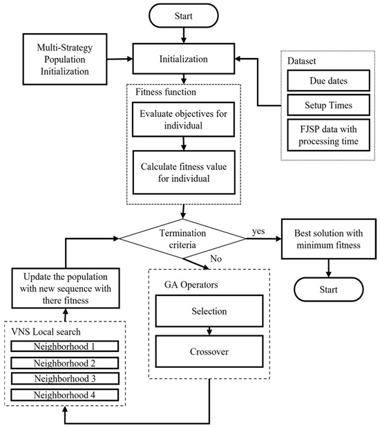
Figure 1.
Flowchart for the proposed algorithm.
The approach to solving the multi-criteria, multi-objective FJSP optimization problem is as follows:
3.1. Multi-Strategy Population
As the population size is limited and problem dimensions are high, the problem becomes promising for obtaining the required search space. In this study, the initial population size is 200, and for every subpopulation, the size is 50. The multi-strategy population approach introduces a diverse set of feasible solutions. To create a well-diversified initial population, multiple dispatching rules are used for the assignments of machines and operation sequencing, which can improve the process of creating near-optimal schedules. It helps to converge faster toward a near-optimal solution. To maintain a better balance between exploration and exploitation, a combination of heuristic rules with randomization approaches helps the algorithm converge faster and improve the quality of the solution to achieve the required solution objective.
P = p1 ∪ p2 ∪ p3 ∪ p4
Equation (9) indicates the initial population produced by four subsets.
Table 6 illustrates four different strategies used for machine selection and operation sequencing to form the population. In p1, both machine selection and operation sequencing are performed randomly, encouraging broad exploration. p2 uses the shortest processing time heuristic for machine selection, with random operation sequencing. p3 uses random selection for machine selection and prioritizes operation sequencing based on a combination of Least Work Remaining (LWKR) and Flow Due Date (FDD) [41]. p4 applies random machine selection and sequencing of the operation using the critical ratio (CR) heuristic [42].
Table 6.
Multi-strategy population approach.
3.2. Fitness Function
In the fitness function, calculate the fitness value of each sequence present in the population. To calculate the fitness of each feasible sequence, it should be scheduled to satisfy all constraints as shown in Equations (2)–(4). After obtaining the makespan, total tardiness, and total setup time values for a sequence, calculate the fitness value using the weighted sum method. The weight is determined by the priority of the criteria. Here, weight is allocated equally, but it can vary based on requirements.
Equation (10) shows how fitness is calculated by the weighted contributions. The weight can vary according to the priority. For this study, ensure that all objectives are treated as equal, so w1 = w2 = w3 = 1/3 while keeping the sum of weights normalized to 1.
3.3. GA Operators
In the framework of the proposed hybrid method, two GA operators, selection and crossover, are utilized in the evolutionary process:
3.3.1. Selection
The selection operator is utilized to choose individual sequences from the population for the next generation. This paper used the random selection method. Initially, any two subsets of a population are selected from which individual sequences are randomly chosen without considering their fitness.
3.3.2. Crossover
In the crossover operation in the GA, two-parent sequences exchange information to create two child sequences. This study proposes the two crossover methods, which are selected randomly over each iteration. The first is a two-point crossover, and the second is a multi-point crossover. The crossover probability is set to 0.8, which ensures diversity in generating offspring.
Equations (15) and (16) show the parent sequences selected by the selection operator. Two points were selected randomly (17). In this, the selected operation from parent 2 has the same job number and operation number as parent 1, which results in two unique child sequences that combine information from both parents.
3.4. Local Search
In this proposed algorithm, the VNS is used as a local search. There are four neighborhood structures used.
- N1 (swap): randomly select two operations from the sequence and swap their positions.
- N2 (reversion): randomly selects two positions from the sequence and reverses all operations between those positions.
- N3 (insertion): two operations are chosen randomly, and the second operation is placed in front of the first.
- N4 (rearrangement): four positions are randomly chosen from the sequence and shuffled in their order.
In this study, new solutions are generated by utilizing the four neighborhood structures. The sequence obtained from the GA operator is used for the VNS local search to escape from the local optima. The local search is applied to vary the order of operations in the job. The detailed steps of VNS are given in Algorithm 1.
| Algorithm 1 Local search |
|
|
|
|
|
|
|
Set |
|
|
3.5. Termination Criteria
After each iteration, the initial population is updated with a new sequence generated by the hybrid GA and VNS algorithms. In the proposed method, 500 iterations are used to obtain a near-optimal solution. The stopping criterion was set to 500 iterations after observing multiple runs of the problem, where the algorithm consistently reached near-optimal solutions for small datasets. For medium or more complex datasets, the number of iterations can be increased beyond 500 according to the dataset size to improve solution quality.
4. Proposed Rescheduling Methods for Dynamic Events
In this section, different dynamic events are discussed using a rescheduling approach within the FJSP with multiple criteria.
4.1. Rescheduling for Job Arrival
Figure 2 shows the workflow for the job arrival dynamic event. In this dynamic event, a new batch of jobs arrives unexpectedly at a particular time while the 1st batch is scheduled. To demonstrate this event, this paper considers flexible processing time with sequence-dependent setup time. In this proposed method, this article used the rescheduling technique, which extracts the required data of the first batch solution and computes with the required data of the second batch. To optimize the solution, the hybrid GAVNS algorithm with a multi-strategy population is used, which is mentioned in the static proposed method.
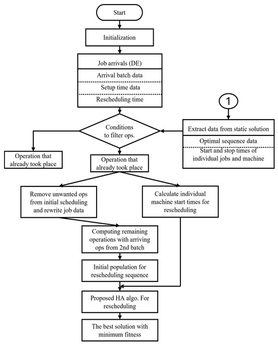
Figure 2.
Flowchart for the job arrival rescheduling strategy.
In the job arrival dynamic event, initialize the method with a second batch of jobs with processing time, sequence-dependent setup time, and rescheduling time, which is the new job’s arrival time. According to conditions, first filter out the first batch operations that have already taken place before the scheduled time, as well as operations that need to be rescheduled with the second batch operation.
The conditions for identifying operations to be included in the rescheduling process are outlined as follows:
- Operations Oi,j that started before the rescheduling time—that is, the start time Si,j of the operation is earlier than the rescheduling time Tresch—will be excluded from the rescheduling process.
Okeep = { Oi,j| (Si,j < Tresch) }
- 2.
- Operations that did not start before the rescheduling time—that is, the start time Si,j of the operation is later than the rescheduling time Tresch—will be included in the rescheduling process.
Oreschedule = { Oi,j| (Si,j ≥ Tresch) }
After eliminating unnecessary operations from the initial static scheduling sequence, the remaining relevant operations are combined with operations from the newly arrived job dataset. Finally, a new computed dataset is prepared for rescheduling, ready to be optimized for a feasible solution. To optimize the solution, this paper utilizes the hybrid GAVNS algorithm with a multi-strategy population, aiming to minimize parameters such as makespan and total setup time, ultimately achieving the best solution with minimum fitness.
4.2. Rescheduling for Machine Breakdown
Figure 3 shows the flowchart of machine breakdown in flexible job shop scheduling. Machine breakdown, referred to as a dynamic event, occurs when a machine unexpectedly fails at a specific point in the schedule.
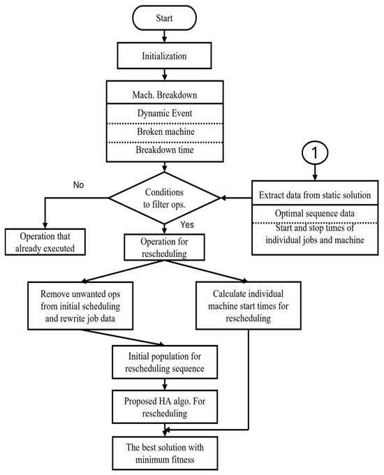
Figure 3.
Flowchart for the machine breakdown rescheduling strategy.
In flexible job shop scheduling, an unforeseen machine failure can cause significant disruptions in the production process, ultimately leading to delays in processing. In the proposed approach, the initial step is to collect essential information about the machine breakdown, such as the specific machine involved and the time of failure. In the next step, filter out the operations according to conditions.
The following conditions are used to determine which operations should be included in the rescheduling process:
- Operations affected by machine breakdown (operations to reschedule):
- 1.
- Operations that extend beyond the breakdown time, that is, when the completion time Ci,j of the operation Oi,j is greater than or equal to the breakdown time Tb, will be included in the rescheduling strategy (Ci,j ≥ Tb).
- 2.
- Operations that started after the breakdown time, that is, when the start time Si,j of the operation Oi,j is greater than the breakdown time Tb, will be included in the rescheduling strategy (Si,j ≥ Tb).
Oreschedule = { Oi,j | (Ci,j ≥ Tb ∨ Si,j ≥ Tb) ∧ Mk ∈ Mb }
- Operations not affected by machine breakdown (operations not to be rescheduled):
- 3.
- Operations that are finished successfully before the breakdown occurs, that is, when the completion time Ci,j of the operation Oi,j is less than the breakdown time Tb, will not be considered in the rescheduling strategy (Ci,j < Tb).
Okeep = { Oi,j | (Ci,j < Tb) ∧ Mk ∉ Mb }
After filtering out non-essential operations, the remaining operations must be rescheduled utilizing the proposed hybrid optimization method. The machines are assigned revised start times to derive an optimized rescheduling sequence, ensuring efficiency and minimal disruption to the overall scheduling process.
5. Results and Discussion
This study presents an analysis of both static and dynamic events, along with their respective analysis.
5.1. Static Flexible Job Shop Scheduling
This section analyzes the performance of the proposed hybrid approach under static conditions, considering two different machine environments.
5.1.1. For a Single-Purpose Machine
The result of the FJSP for the single-purpose machine environment is considered by considering the makespan, total setup time, and total tardiness. To demonstrate this event, the dataset we used is mentioned in the multi-purpose machine environment section. Figure 4 shows the Gantt chart for scheduling 17 jobs using a proposed hybrid framework.
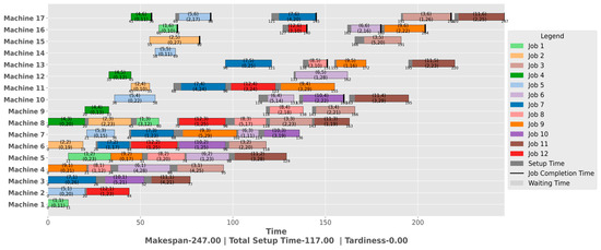
Figure 4.
Gantt chart of static scheduling for 17 jobs.
After applying the proposed hybrid algorithm, the solutions demonstrate a significant improvement in objective performance. As shown in Figure 5, the makespan decreased from 289 to 247 units, while the total setup time was reduced from 164 units to 117 units. The total tardiness achieved its optimal value from 149 to 0 over the iteration. This indicates that all jobs finished before their due dates listed in Table 5, and no job was delayed. The overall fitness value has decreased from 172 to 103 over the iteration.
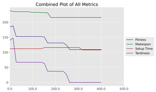
Figure 5.
Minimization of fitness, makespan, setup time, and tardiness over iterations.
As shown in Table 7, single-purpose machine datasets are used to evaluate the performance of the proposed method compared to the genetic approach. Also mention iteration size for each problem by considering the size of the data.
Table 7.
Comparison results.
The datasets were used for evaluating the proposed algorithm under different problem sizes. Each dataset instance is denoted as SPM_FJSP_XjxYmg, where Xj represents the number of jobs and Ymg indicates the number of considered machine groups. The proposed method outperformed the GA approach on 10 out of 11 datasets, achieving up to 5.60% improvement. The average improvement across all datasets is 2.59%, which confirms the robustness and efficiency of the proposed approach in minimizing fitness value across a variety of configurations.
5.1.2. For a Multi-Purpose Machine
The results of the FJSP problem are obtained by considering the criteria of due date, setup time, and processing time. The three objectives include minimizing total tardiness, minimizing total setup time, and minimizing makespan.
Figure 6 shows the result of the FJSP with a Gantt chart. The completion time for job 1 is 55 units, with a due date of 57 units, which means it was completed 2 units before the deadline. Another job took 75 units of time to complete; it had a due date of 72 units, resulting in a tardiness of 3 units. Job 3 was completed before the deadline, as its due date is 54 units, but it was completed in 39 units of time. The fourth job due date is 79 units, and it has been completed at 86 units, which means the tardiness of job 4 is 7. The total tardiness becomes 10 units. The total setup time is 10, with a makespan of 86 units. As shown in Figure 7, the fitness levels dropped from 60 to 35.8, which is a reduction of 40.33%.
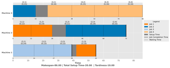
Figure 6.
Gantt chart results for 4-by-3 data.
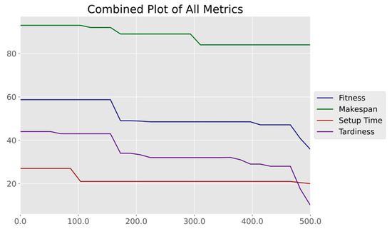
Figure 7.
Minimization of fitness, makespan, setup time, and tardiness over iterations.
Table 8 shows the comparison result of the fitness value. The proposed method is compared with various methods: A1, which is 2PT + LWR + FDD; A2, which is 2PT + LWR + Slack; A3, which is 2PT + LWR + EDD [18]; and GA [26]. After comparison of all Brandimarte datasets with an extension of the due date and setup time, an overall 6.51% improvement result was obtained. Table 8 illustrates the comparison between the proposed algorithm and other existing methods regarding the number of best results obtained, also stopping criterion of iteration size is decided by considering the size of the dataset mentioned. This validates the effectiveness of the proposed method in optimizing the flexible job shop scheduling problem. The fitness value is calculated by giving the same weight to all objectives. For the proposed algorithm, the value of makespan (MK), total setup time (TST), and total tardiness (TT) are mentioned.
Table 8.
Comparison result.
5.2. Dynamic Flexible Job Shop Scheduling
This section discusses dynamic events such as machine breakdowns and job arrivals.
5.2.1. Job Arrival
In this section, the arrival of an urgent job is considered a dynamic event. In real-world manufacturing systems, it is common for urgent jobs to arrive after the initial schedule has started for production, so at any time during static scheduling, urgent jobs are introduced.
In this dynamic event, consider the processing time and setup time. In this experiment, three new jobs (job 5, job 6, and job 7) are considered as the second batch, with their corresponding processing times given in Table 9. Consider that the second batch arrives at the 48-unit mark.
Table 9.
FJSP dataset with 3 jobs and 3 machines.
After following the static schedule, the first batch processed using the proposed hybrid algorithm achieved a makespan of 78 units, as illustrated in Figure 8. The second batch of jobs was then rescheduled at the 48-unit marked in red line, as shown in Figure 9. When an urgent batch of jobs arrives, the system must reschedule the all jobs after time 48 from the first batch including all jobs from the urgent batch. The jobs that already started before the rescheduling time (48 units) should not be disturbed, so the jobs J(4,3), J(2,2), and J(3,13) will not participate in rescheduling, but other jobs from batch one that started after the rescheduling time, such as J(4,4), J(2,3), J(2,4), and J(3,3), will participate in rescheduling with new jobs and form the new optimal solution by optimizing the proposed hybrid framework. The operations of the first batch that participate in rescheduling change their sequence for an optimal solution, which gives the minimal makespan with minimal total setup time. Operations 2, 3, and 4 from job 6 are processed back-to-back, so the setup time is not required, which is achieved using the proposed hybrid framework having the GA, VNS, and an initial population strategy.
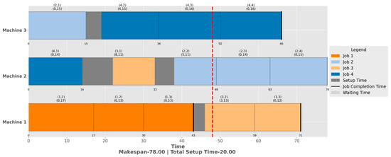
Figure 8.
Gantt chart for static scheduling.
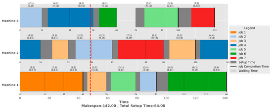
Figure 9.
Gantt chart for rescheduling after 3 arrival jobs.
5.2.2. Machine Breakdown
Machine breakdowns are common in real production environments and disturb the ongoing schedule. To demonstrate machine breakdown, a machine breakdown is performed on static scheduling, which is shown in Figure 10, showing the Gantt chart for static scheduling for three machines and four jobs using FJSP data. The data include the sequence-dependent setup time that is available in Table 2. Figure 11 shows the rescheduling after the third machine breakdown at 40 time units, which is mentioned in the dotted red line. On machine 3, the operations that are not completed because of unexpected machine failure will participate in the rescheduling scheme. Other operations on other machines after the breakdown time and operations that have already started will be completed without interruption, but the operations that have not started after the breakdown time will participate in the rescheduling. In rescheduling, selected operations are scheduled using the proposed hybrid algorithm, which will be capable of reaching a near-optimal solution for rescheduling. After breaking down the third machine, the operation J(4,3) remains incomplete, which is why it will again be rescheduled for the new optimal sequence. On the other hand, the operation that has already started on other machines (m1,m2), such as J(2,2) and J(1,3), can proceed successfully with interruption or rescheduling. The operation J(4,3), J(4,4) from the breakdown machine after breakdown time, and J(2,3), J(2,4), J(3,13), and J(3,3) from other machines will be rescheduled to obtain the best possible solution.
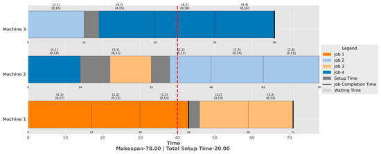
Figure 10.
Gantt chart for scheduling before machine breakdown.
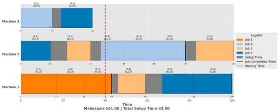
Figure 11.
Gantt chart for rescheduling after machine breakdown.
Table 10 presents a comparative study of different scheduling approaches and their characteristics. The comparison includes various characteristics such as JSP, FJSP, and multi-criteria, like processing time, setup time, dispatching rules/priority rules, heuristic algorithms, job arrival handling, and machine breakdown handling.
Table 10.
Comparative study.
The FJSP is the extended version of the JSP, which offers more flexibility in the choice of machines with processing time. Some articles do not consider criteria like setup time, which is included in this study. Many studies have proposed only dispatching rules or heuristic algorithms. Nowhere in these studies has an algorithm been proposed that combines hybrid heuristic algorithms with priority rules, which gives better results. Job arrival and machine breakdown are the main dynamic events that often occur in manufacturing factories where scheduling is the task.
6. Conclusions
The flexible job shop problem (FJSP) is a key challenge in manufacturing systems, where effective management of processing times, setup times, and due dates is critical for efficient production. These factors play a major role in determining how well manufacturing processes can meet their targets while minimizing delays and costs. In this study, we have proposed a hybrid scheduling algorithm designed to address the complexities of the FJSP by combining multiple strategies. Our approach begins with a diverse set of initial solutions created through a genetic algorithm, followed by a local search method known as variable neighborhood search (VNS) to fine-tune the solutions for optimal results.
In the case of static scheduling, where the problem does not change over time, our algorithm demonstrated a 6.5% improvement in fitness. This result shows that the hybrid method is effective in enhancing the overall scheduling performance. Moving on to dynamic scheduling, which introduces additional complexity like sudden job arrivals or unexpected machine breakdowns, we applied a rescheduling approach that led to a significant reduction in makespan. This is particularly important in real-world manufacturing environments where unpredictability can heavily impact production efficiency.
To validate the performance of our approach, we compared it to the well-known genetic algorithm (GA) using a variety of benchmark datasets based on the FJSP. The results were promising. Out of 11 different tested instances, our method outperformed the GA in 9 cases, matched its performance in 1 case, and was only slightly outperformed in 1 case. These comparisons demonstrate that the proposed hybrid algorithm consistently provides better or comparable results, offering a strong alternative to existing solutions.
One of the most notable findings from this research is the average improvement of 2.59% in makespan, which highlights the effectiveness of the proposed method, particularly when applied to more complex instances involving multiple jobs and machine groups. This improvement is a significant step toward achieving more efficient and flexible job shop scheduling in manufacturing systems.
The success of our proposed method in minimizing key objectives, such as processing time, setup time, and due dates, confirms that it can handle the multiple competing factors that make scheduling in manufacturing so difficult. By addressing both static and dynamic scheduling scenarios, our algorithm provides a comprehensive solution that can adapt to the evolving needs of a manufacturing environment.
In conclusion, the results of this study underscore the potential of the proposed hybrid scheduling approach to enhance manufacturing system performance. By offering improved scheduling outcomes, the method not only demonstrates its practicality in real-world settings but also contributes valuable insights for future research in this field. The novelty of this work lies in the integrated GA and VNS, applying a multi-strategy population initialization scheme, and extending standard benchmark datasets for two different environments with multi-objectives, such as minimizing makespan, minimizing total tardiness, minimizing total setup time, and multi-criteria of due dates and sequence-dependent setup time, which sustainably provide the rescheduling for the dynamic events. The hybrid algorithm’s ability to effectively balance multiple objectives while addressing the dynamic nature of job shop scheduling makes it a promising tool for optimizing manufacturing operations.
Author Contributions
Conceptualization, C.S.K.; designed algorithm, S.K.F. and C.S.K.; supervision, C.S.K.; preprocessed and analyzed the data S.K.F.; wrote the paper, S.K.F.; methodology, S.K.F.; formal analysis, S.K.F.; writing—original draft preparation, S.K.F.; writing—review and editing, S.K.F. and C.S.K.; visualization, S.K.F.; funding acquisition, C.S.K. All authors have read and agreed to the published version of the manuscript.
Funding
This research was supported by the Basic Science Research Program through the National Research Foundation of Korea (NRF), funded by the Ministry of Education (2021R1I1A3052605).
Data Availability Statement
The original contributions presented in this study are included in the article. Further inquiries can be directed to the corresponding author.
Conflicts of Interest
The authors declare no conflicts of interest.
References
- Fattahi, P.; Fallahi, A. Dynamic Scheduling in Flexible Job Shop Systems by Considering Simultaneously Efficiency and Stability. CIRP J. Manuf. Sci. Technol. 2010, 2, 114–123. [Google Scholar] [CrossRef]
- Türkyılmaz, A.; Şenvar, Ö.; Ünal, İ.; Bulkan, S. A Research Survey: Heuristic Approaches for Solving Multi Objective Flexible Job Shop Problems. J. Intell. Manuf. 2020, 31, 1949–1983. [Google Scholar] [CrossRef]
- Baykasoǧlu, A. Linguistic-Based Meta-Heuristic Optimization Model for Flexible Job Shop Scheduling. Int. J. Prod. Res. 2002, 40, 4523–4543. [Google Scholar] [CrossRef]
- Xie, J.; Gao, L.; Peng, K.; Li, X.; Li, H. Review on Flexible Job Shop Scheduling. IET Collab. Intell. Manuf. 2019, 1, 67–77. [Google Scholar] [CrossRef]
- Zhang, S.; Wang, S. Flexible Assembly Job-Shop Scheduling with Sequence-Dependent Setup Times and Part Sharing in a Dynamic Environment: Constraint Programming Model, Mixed-Integer Programming Model, and Dispatching Rules. IEEE Trans. Eng. Manag. 2018, 65, 487–504. [Google Scholar] [CrossRef]
- Blackstone, J.H.; Phillips, D.T.; Hogg, G.L. A State-of-the-Art Survey of Dispatching Rules for Manufacturing Job Shop Operations. Int. J. Prod. Res. 1982, 20, 27–45. [Google Scholar] [CrossRef]
- Holthaus, O.; Rajendranb, C. Efficient Dispatching Rules for Scheduling in a Job Shop. Int. J. Prod. Econ. 1997, 48, 87–105. [Google Scholar] [CrossRef]
- Shi, X.; Long, W.; Li, Y.; Deng, D. Multi-Population Genetic Algorithm with ER Network for Solving Flexible Job Shop Scheduling Problems. PLoS ONE 2020, 15, e0233759. [Google Scholar] [CrossRef]
- Shady, S.; Kaihara, T.; Fujii, N.; Kokuryo, D. Evolving Dispatching Rules Using Genetic Programming for Multi-Objective Dynamic Job Shop Scheduling with Machine Breakdowns. Procedia CIRP 2021, 104, 411–416. [Google Scholar] [CrossRef]
- Ozturk, G.; Bahadir, O.; Teymourifar, A. Extracting Priority Rules for Dynamic Multi-Objective Flexible Job Shop Scheduling Problems Using Gene Expression Programming. Int. J. Prod. Res. 2019, 57, 3121–3137. [Google Scholar] [CrossRef]
- Cheung, W.; Zhou, H. Using Genetic Algorithms and Heuristics for Job Shop Scheduling with Sequence-Dependent Setup Times. Ann. Oper. Res. 2001, 107, 65–81. [Google Scholar] [CrossRef]
- Özgüven, C.; Yavuz, Y.; Özbakir, L. Mixed Integer Goal Programming Models for the Flexible Job-Shop Scheduling Problems with Separable and Non-Separable Sequence Dependent Setup Times. Appl. Math. Model. 2012, 36, 846–858. [Google Scholar] [CrossRef]
- dos Santos, F.; Costa, L.; Varela, L. Multi-Objective Optimization of the Job Shop Scheduling Problem on Unrelated Parallel Machines with Sequence-Dependent Setup Times; Springer Nature: Cham, Switzerland, 2023; Volume 14105, LNCS; ISBN 9783031371073. [Google Scholar]
- Ortíz-Barrios, M.; Petrillo, A.; De Felice, F.; Jaramillo-Rueda, N.; Jiménez-Delgado, G.; Borrero-López, L. A Dispatching-Fuzzy Ahp-Topsis Model for Scheduling Flexible Job-Shop Systems in Industry 4.0 Context. Appl. Sci. 2021, 11, 5107. [Google Scholar] [CrossRef]
- Thenarasu, M.; Rameshkumar, K.; Di Mascolo, M.; Anbuudayasankar, S.P. Multi-Criteria Scheduling of Realistic Flexible Job Shop: A Novel Approach for Integrating Simulation Modelling and Multi-Criteria Decision Making. Int. J. Prod. Res. 2024, 62, 336–358. [Google Scholar] [CrossRef]
- Liu, N.; Qin, K. Research on Improved Genetic Algorithm Based on Multi-Objective Optimization for Flexible Shop Scheduling Problem. In Proceedings of the 2025 5th International Conference on Sensors and Information Technology (ICSI 2025), Nanjing, China, 21–23 March 2025; pp. 719–722. [Google Scholar] [CrossRef]
- He, A.; Liu, X.; Gong, G.; Yuan, Z.; Huang, H.; Zhou, Y.; Li, J. Multi-Objective Optimization for Distributed Flexible Job Shop Scheduling Problem with Job Priority. Swarm Evol. Comput. 2025, 98, 102075. [Google Scholar] [CrossRef]
- Sels, V.; Gheysen, N.; Vanhoucke, M. A Comparison of Priority Rules for the Job Shop Scheduling Problem under Different Flow Time- and Tardiness-Related Objective Functions. Int. J. Prod. Res. 2012, 50, 4255–4270. [Google Scholar] [CrossRef]
- Rahmati, S.H.A.; Zandieh, M.; Yazdani, M. Developing Two Multi-Objective Evolutionary Algorithms for the Multi-Objective Flexible Job Shop Scheduling Problem. Int. J. Adv. Manuf. Technol. 2013, 64, 915–932. [Google Scholar] [CrossRef]
- Draz, U.; Ali, T.; Yasin, S.; Chaudary, M.H.; Ayaz, M.; Aggoune, E.H.M.; Yasin, I. Hybridization and Optimization of Bio and Nature-Inspired Metaheuristic Techniques of Beacon Nodes Scheduling for Localization in Underwater IoT Networks. Mathematics 2024, 12, 3447. [Google Scholar] [CrossRef]
- Tay, J.C.; Ho, N.B. Evolving Dispatching Rules Using Genetic Programming for Solving Multi-Objective Flexible Job-Shop Problems. Comput. Ind. Eng. 2008, 54, 453–473. [Google Scholar] [CrossRef]
- Lunardi, W.T.; Birgin, E.G.; Ronconi, D.P.; Voos, H. Metaheuristics for the Online Printing Shop Scheduling Problem. Eur. J. Oper. Res. 2021, 293, 419–441. [Google Scholar] [CrossRef]
- Fuladi, S.K.; Kim, C.S. Dynamic Events in the Flexible Job-Shop Scheduling Problem: Rescheduling with a Hybrid Metaheuristic Algorithm. Algorithms 2024, 17, 142. [Google Scholar] [CrossRef]
- Ben Ali, K.; Bechikh, S.; Louati, A.; Louati, H.; Kariri, E. Dynamic Job Shop Scheduling Problem with New Job Arrivals Using Hybrid Genetic Algorithm. IEEE Access 2024, 12, 85338–85354. [Google Scholar] [CrossRef]
- Tariq, A.; Khan, S.A.; But, W.H.; Javaid, A.; Shehryar, T. An IoT-Enabled Real-Time Dynamic Scheduler for Flexible Job Shop Scheduling (FJSS) in an Industry 4.0-Based Manufacturing Execution System (MES 4.0). IEEE Access 2024, 12, 49653–49666. [Google Scholar] [CrossRef]
- Ben Ali, K.; Telmoudi, A.J.; Gattoufi, S. An Improved Genetic Algorithm with Local Search for Solving the DJSSP with New Dynamic Events. In Proceedings of the IEEE 23rd International Conference on Emerging Technologies and Factory Automation (ETFA), Torino, Italy, 4–7 September 2018; pp. 1137–1144. [Google Scholar] [CrossRef]
- Thi, L.M.; Mai Anh, T.T.; Van Hop, N. An Improved Hybrid Metaheuristics and Rule-Based Approach for Flexible Job-Shop Scheduling Subject to Machine Breakdowns. Eng. Optim. 2023, 55, 1535–1555. [Google Scholar] [CrossRef]
- Ding, L.; Guan, Z.; Luo, D.; Rauf, M.; Fang, W. An Adaptive Search Algorithm for Multiplicity Dynamic Flexible Job Shop Scheduling with New Order Arrivals. Symmetry 2024, 16, 641. [Google Scholar] [CrossRef]
- Pezzella, F.; Morganti, G.; Ciaschetti, G. A Genetic Algorithm for the Flexible Job-Shop Scheduling Problem. Comput. Oper. Res. 2008, 35, 3202–3212. [Google Scholar] [CrossRef]
- Azzouz, A.; Ennigrou, M.; Ben Said, L. Flexible Job-Shop Scheduling Problem with Sequence-Dependent Setup Times Using Genetic Algorithm. In Proceedings of the ICEIS 2016—18th International Conference on Enterprise Information Systems, Rome, Italy, 25–28 April 2016; Volume 2, pp. 47–53. [Google Scholar] [CrossRef][Green Version]
- Huang, X.; Yang, L. A Hybrid Genetic Algorithm for Multi-Objective Flexible Job Shop Scheduling Problem Considering Transportation Time. Int. J. Intell. Comput. Cybern. 2019, 12, 154–174. [Google Scholar] [CrossRef]
- Türkylmaz, A.; Bulkan, S. A Hybrid Algorithm for Total Tardiness Minimisation in Flexible Job Shop: Genetic Algorithm with Parallel VNS Execution. Int. J. Prod. Res. 2015, 53, 1832–1848. [Google Scholar] [CrossRef]
- Wang, Y.; Zhu, Q. A Hybrid Genetic Algorithm for Flexible Job Shop Scheduling Problem with Sequence-Dependent Setup Times and Job Lag Times. IEEE Access 2021, 9, 104864–104873. [Google Scholar] [CrossRef]
- Sun, K.; Zheng, D.; Song, H.; Cheng, Z.; Lang, X.; Yuan, W.; Wang, J. Hybrid Genetic Algorithm with Variable Neighborhood Search for Flexible Job Shop Scheduling Problem in a Machining System. Expert Syst. Appl. 2023, 215, 119359. [Google Scholar] [CrossRef]
- Ojstersek, R.; Tang, M.; Buchmeister, B. Due Date Optimization in Multi-Objective Scheduling of Flexible Job Shop Production. Adv. Prod. Eng. Manag. 2020, 15, 481–492. [Google Scholar] [CrossRef]
- Ho, N.B.; Tay, J.C. Evolving Dispatching Rules for Solving the Flexible Job-Shop Problem. In Proceedings of the 2005 IEEE Congress on Evolutionary Computation (IEEE CEC 2005), Edinburgh, Scotland, 2–5 September 2005; Volume 3, pp. 2848–2855. [Google Scholar] [CrossRef]
- Ojstersek, R.; Palcic, I.; Buchmeister, B. Production Scheduling Using Twk and Slk Methods. Ann. DAAAM Proc. 2021, 32, 228–234. [Google Scholar] [CrossRef]
- Rahman, H.F.; Janardhanan, M.N.; Poon Chuen, L.; Ponnambalam, S.G. Flowshop Scheduling with Sequence Dependent Setup Times and Batch Delivery in Supply Chain. Comput. Ind. Eng. 2021, 158, 107378. [Google Scholar] [CrossRef]
- Madhav, S.; Ahamad, A.; Singh, P.; Mishra, P.K. A Review of Textile Industry: Wet Processing, Environmental Impacts, and Effluent Treatment Methods. Environ. Qual. Manag. 2018, 27, 31–41. [Google Scholar] [CrossRef]
- Meng, L.; Cheng, W.; Zhang, B.; Zou, W.; Duan, P. A Novel Hybrid Algorithm of Genetic Algorithm, Variable Neighborhood Search and Constraint Programming for Distributed Flexible Job Shop Scheduling Problem. Int. J. Ind. Eng. Comput. 2024, 15, 813–832. [Google Scholar] [CrossRef]
- Jayamohan, M.S.; Rajendran, C. New Dispatching Rules for Shop Scheduling: A Step Forward. Int. J. Prod. Res. 2000, 38, 563–586. [Google Scholar] [CrossRef]
- Chiang, T.C.; Fu, L.C. Using a Family of Critical Ratio-Based Approaches to Minimize the Number of Tardy Jobs in the Job Shop with Sequence Dependent Setup Times. Eur. J. Oper. Res. 2009, 196, 78–92. [Google Scholar] [CrossRef]


Disclaimer/Publisher’s Note: The statements, opinions and data contained in all publications are solely those of the individual author(s) and contributor(s) and not of MDPI and/or the editor(s). MDPI and/or the editor(s) disclaim responsibility for any injury to people or property resulting from any ideas, methods, instructions or products referred to in the content. |
© 2025 by the authors. Licensee MDPI, Basel, Switzerland. This article is an open access article distributed under the terms and conditions of the Creative Commons Attribution (CC BY) license (https://creativecommons.org/licenses/by/4.0/).