Abstract
To address the challenge of identifying water-flooded layers in the high-porosity, high-permeability, and strongly heterogeneous reservoirs of the Guantao Formation in the Penglai 19-3 Oilfield, research on water-flooded layer identification methods was systematically conducted. The logging characteristics of oil layers and water-flooded layers at different levels overlap considerably, which limits the accuracy of traditional identification methods. Meanwhile, the Archie equation shows significantly reduced applicability during the moderate and strong water-flooding stages. A water-flooded layer identification model was constructed using HistGBDT, and performance comparison between the base model and the optimized model reveals that the latter achieves a test accuracy of 91.6%. Compared with BPNN and SVM, the optimized HistGBDT model demonstrates substantially higher test accuracy and better generalization performance. Based on six sets of logging data, the optimized HistGBDT model developed enables the accurate identification of oil layers and multi-level water-flooded layers. It provides a reliable technical approach for tapping remaining oil in the high-water-cut stage of the Penglai 19-3 Oilfield and offers a new method and engineering reference for water-flooded layer identification in similar high-porosity, high-permeability heterogeneous reservoirs in the Bohai Bay Basin.
1. Introduction
Offshore oil and gas resources, as crucial components of global energy supply, are of strategic significance for ensuring energy security through their efficient development. The Bohai Bay Basin, an important petroliferous basin in eastern China, has nurtured multiple large-scale offshore oilfields. Among these, the Penglai 19-3 Oilfield, with its geologically recoverable crude oil resources ranging from 108 to 109 tons, stands as one of the largest offshore integrated oilfields in the Bohai Bay Basin and occupies a core position in China’s offshore oil and gas development system [1]. Located in the central–southern part of the Bohai Sea, the oilfield lies in the upper part of the Bonan Uplift at the northeastern end of the Bohai Bay Basin. Controlled by the Tan-Lu fault zone and the adjacent strike–slip tectonic system, it exhibits an overall anticlinal uplift morphology with well-developed faults. The complex tectonic setting has given rise to unique reservoir characteristics and development challenges [2].
The study area belongs to the Neogene Guantao Formation (N1g) of the Penglai 19-3 Oilfield, which serves as one of the major pay zones of the oilfield. Belonging to a continental fluvial-delta sedimentary system, this formation has established the basic sedimentary framework of the reservoirs. The reservoirs are dominated by continental clastic sandstones, commonly featuring coronally long-distance channel sandbodies and channel sandbodies deposited by braided river deltas. Lithologies primarily range from siltstone-medium sandstone to coarse sandstone with high feldspar content, intercalated with argillaceous and silty interbeds. The caprock system consists mainly of relatively continuous mudstones and siltstones that form effective sealing [2]. Multiple phases of tectonic activities have significantly modified the reservoirs in terms of fractures and pores, directly affecting the sealing capacity of the reservoir and oil–gas supply capacity.
In contrast, neotectonic activities have ensured the continuous late-stage charging of oil and gas. The coupling of tectonic and sedimentary processes has formed multiple sets of composite reservoir–caprock assemblages. The unique sedimentary and tectonic settings endow the reservoirs with distinct high-porosity and high-permeability characteristics: the average porosity reaches 20.21%, with some intervals even up to 32.9%, and the average permeability is 708.01 mD, ranging from several millidarcies to thousands of millidarcies, which easily form extremely high-permeability channels. However, significant differences in reservoir physical properties, firm lateral and vertical heterogeneity, and significant variations in connectivity pose severe challenges to the identification of water-flooded layers during reservoir development.
Water-flooded layer identification constitutes a core technical link in the middle and late stages of oil and gas field development, and its accuracy is directly related to the prediction of remaining oil distribution, adjustment of development plans, and improvement of oil recovery [3,4,5]. In high-porosity, high-permeability heterogeneous reservoirs such as those in the Penglai 19-3 Oilfield, water injection development, as the primary means to maintain formation pressure and enhance oil recovery, inevitably leads to gradual water flooding of oil layers. With the intensification of water flooding, a series of changes occur in reservoirs’ physical and chemical properties, and fluid distribution and pore structure undergo continuous reconstruction, which sharply increases the difficulty in identifying oil and water-flooded layers at different levels [6,7,8]. Traditional water-flooded layer identification mainly relies on logging response characteristic analysis and quantitative models such as the Archie equation. However, the limitations of these methods have become increasingly prominent under the complex reservoir conditions of the study area.
In terms of logging response characteristics, significant interference exists in identifying water-flooded and oil layers in the study area. Although the gamma ray curve shows a decreasing trend in water-flooded layers, reflecting that some radioactive substances remain unremoved after oil layer flooding, it can only serve as an auxiliary indicator for water-flooded layer identification. As a fluid-sensitive indicator, the resistivity curve exhibits differences under different water flooding levels: the resistivity of oil layers is greater than 8–20 Ω·m, that of strongly water-flooded layers is 2–5 Ω·m, moderately water-flooded layers is 4–6 Ω·m, and weakly water-flooded layers is 10–16 Ω·m. However, the resistivity of weakly water-flooded layers differs slightly from that of oil layers, easily leading to misjudgment. More critically, density and compensated neutron logging responses overlap significantly between oil and water-flooded layers. This overlapping of response characteristics makes it difficult for single or combined logging curves to differentiate accurately between oil and water-flooded layers at different levels.
The Archie equation, a quantitative model establishing the relationship between resistivity and oil saturation based on pure sandstone reservoirs [9,10,11], has been widely applied in water-flooded layer identification in homogeneous reservoirs. Its core expression links formation resistivity to oil saturation through parameters such as lithology coefficient, cementation exponent, and saturation exponent [11]. However, water flooding of oil layers disrupts the physical and chemical equilibrium of the original reservoir, fundamentally undermining the application basis of the Archie equation. The application of this equation requires three prerequisites: the reservoir is pure sandstone without additional conductive effects, oil and water phases in pores are uniformly distributed, and the reservoir cementation state is stable with pore structure unchanged by water injection. In the study area, however, during the moderate and strong water-flooding stages, water injection causes swelling of clay minerals (montmorillonite, illite), forming a conductive network of clay-bound water and intensifying additional conductive responses, resulting in measured resistivity lower than the theoretical resistivity of pure sandstone; long-term water injection scouring leads to cement dissolution and deteriorated particle sorting, forming complex pore structures with both macropores and microvoids, which is inconsistent with the uniform pore type assumed by the Archie equation; meanwhile, non-uniform filling of residual oil in pores enhances the heterogeneity of fluid distribution. These changes significantly reduce the applicability of the Archie equation in moderately and strongly water-flooded layers with sharply increased errors, and only retain specific applicability in weakly water-flooded layer identification, where lithology and pore structure have not changed significantly.
Core data calibration, as an important basis for verifying and optimizing water-flooded layer identification methods, also faces multiple limitations in the study area. After water flooding, reservoir cements swell upon contact with water and their strength decreases, making wellbore walls prone to collapse during coring, leading to broken and missing cores with low recovery rate and poor integrity; limited by the size of coring tools, water-flooded layers with thickness less than 0.5 m are prone to missed coring or layer mixing; more critically, the imbalance between wellbore pressure and reservoir pressure during coring causes volatilization of light components of crude oil in cores and overflow of formation water, while clay mineral swelling further damages the pore structure. These issues make it challenging to preserve core fluids, resulting in significant deviations of physical parameters such as porosity and permeability from the original underground state, which fails to provide reliable calibration data for identification models.
To break through the bottlenecks of traditional methods in water-flooded layer identification in complex reservoirs, machine learning technology has become a research hotspot in recent years due to its strong multivariate nonlinear mapping capability and small-sample learning advantage [12,13,14]. Machine learning can integrate multi-source logging data, automatically mine the implicit correlation between logging responses and water-flooding levels, and solve problems such as scarce coring data, easy fluid distortion, and poor adaptability to heterogeneous reservoirs, reducing production costs and improving analysis efficiency. In the field of water-flooded layer identification, random forests are suitable for multi-source heterogeneous data integration due to their feature screening and anti-overfitting capabilities; gradient boosting decision trees (XGBoost/LightGBM) focus on high-precision fitting with small samples [15,16,17]; BP neural networks excel at processing nonlinear mapping relationships; and support vector machines are applied to the identification of thin layers and low-resistivity reservoirs [12,18,19,20]. Among these, the gradient boosting decision tree algorithm is highly compatible with the data conditions of the study area due to its excellent performance in small-sample scenarios.
As an optimized evolution of gradient boosting decision trees, the HistGBDT maps continuous features into histograms for split decision-making, significantly reducing computational complexity and memory usage. Its efficiency is improved by more than 30% compared with traditional XGBoost, perfectly solving the time-consuming problem in multi-parameter integration [21,22,23]; meanwhile, the discretization of histograms naturally enhances the model’s robustness to noisy data. In fragmented data scenarios such as high-water-cut unconsolidated reservoirs, its anti-overfitting capability is superior to ordinary gradient boosting decision trees, enabling more accurate screening of key features such as the ratio of deep to medium lateral resistivity; in addition, its efficient utilization of small-sample data can further reduce reliance on core calibration data, endowing it with unique advantages in reservoirs with high porosity, high permeability, firm heterogeneity, and thin layers where coring data is scarce.
Notably, the performance improvement of the HistGBDT model is inseparable from parameter optimization, and significant differences exist in identification effects between the base model and the optimized model. Parameters of the base model (such as the number of iterations and tree depth) are mainly preset based on manual experience, without fully considering the distribution characteristics of logging data and sample balance, and lack a cross-validation link. This makes the model vulnerable to the randomness of data splitting, resulting in limited generalization ability. In contrast, the optimized model constructs a grid of core parameters, including the number of iterations, tree depth, learning rate, and minimum number of samples in leaf nodes, through GridSearchCV, covering 36 parameter combinations. The optimal configuration is selected with 3-fold cross-validation, ultimately achieving comprehensive improvement in core indicators and effectively solving the problems of sample imbalance and parameter adaptation, thus providing a more reliable model basis for accurate identification.
Meanwhile, the optimized HistGBDT model demonstrates more prominent technical advantages than traditional machine learning methods. A multi-dimensional comparison with BPNN and SVM shows that in terms of prediction accuracy, the test accuracy of HistGBDT reaches 0.92, far exceeding BPNN and SVM, and its F1-score is 11 percentage points and 17 percentage points higher than the two respectively; in terms of generalization ability, its generalization accuracy is 0.88 with a cross-validation standard deviation of only 0.01, which is 1/3 of that of BPNN and SVM, indicating better stability. HistGBDT can trace the identification logic through feature importance and decision path visualization. BPNN and SVM exhibit “black-box” characteristics that cannot meet the demand for result interpretability in engineering practice. In addition, BPNN is prone to falling into local minima and has strict requirements for data preprocessing [18], while SVM is likely to produce class imbalance errors in multi-classification scenarios. HistGBDT effectively avoids these defects and is more suitable for identification tasks in complex reservoirs [12,16].
Based on the above research background and technical status, research on the application of the HistGBDT model in water-flooded layer identification was systematically conducted, taking the Neogene Guantao Formation reservoir of the Penglai 19-3 Oilfield as the research object to address the identification challenges caused by high porosity, high permeability, and firm heterogeneity. Firstly, the geological background and reservoir characteristics of the study area were elaborated to clarify the geological challenges faced by water-flooded layer identification; secondly, logging response characteristics were analyzed to reveal the limitations of traditional identification methods; further, the causes for the reduced applicability of the Archie equation were discussed to provide a theoretical basis for model selection; on this basis, a base HistGBDT model was constructed based on six sets of logging data including GR, RDEEP, and RMED, and an optimized model was obtained through GridSearchCV parameter optimization and cross-validation. Differences between the two models in core indicators such as accuracy and F1-score, as well as in the identification effect of small samples, were systematically compared; meanwhile, comprehensive comparison between the optimized HistGBDT model, BPNN, and SVM was conducted in terms of prediction accuracy, generalization ability, and interpretability to verify its technical advantages; finally, the identification accuracy and applicability of the optimized HistGBDT model under complex reservoir conditions were clarified. This study aims to provide a new method and technical reference for water-flooded layer identification in similar high-porosity, high-permeability heterogeneous reservoirs in the Bohai Bay Basin, and contribute to improving oil recovery in the middle and late stages of offshore oilfield development.
2. Materials and Methods
2.1. Geological Setting
The Penglai 19-3 Oilfield, one of the largest offshore oilfields in the Bohai Bay Basin, is a large-scale integrated oilfield with geologically recoverable crude oil resources ranging from 108 to 109 tons. It exhibits distinct shallow offshore coastal geographical characteristics: located in the central–southern part of the Bohai Sea, it lies in the upper part of the uplift at the northeastern end of the Bohai Bay Basin (see Figure 1) [2]. Tectonically controlled by the Tan-Lu fault zone and the adjacent strike–slip tectonic system, the oilfield is situated at the northeastern end of the Bonan Uplift and presents an overall anticlinal uplift morphology with well-developed faults. Multiple phases of tectonic activities have modified the reservoir fractures and pores, directly affecting the sealing capacity of the reservoir and oil–gas supply capacity. The coupling of tectonic and sedimentary processes has formed multiple sets of composite reservoir–caprock assemblages, where effective sealing systems are composed of multiple sets of sandbodies and interbedded mudstones. Neotectonic activities have ensured the continuous late-stage charging of oil and gas.
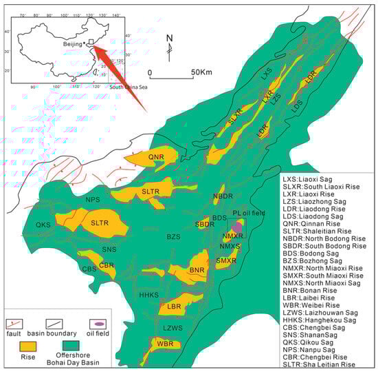
Figure 1.
Regional location [2].
The study area belongs to the Neogene Guantao Formation (N1g), one of the major pay zones of the oilfield. Belonging to a continental fluvial-delta sedimentary system, this formation has established the basic sedimentary framework of the reservoirs. The reservoirs are dominated by continental clastic sandstones, commonly featuring coronally long-distance channel sandbodies and channel sandbodies deposited by braided river deltas. Lithologies primarily range from siltstone-medium sandstone to coarse sandstone with high feldspar content, intercalated with argillaceous and silty interbeds. The caprock is mainly composed of relatively continuous mudstones and siltstones. Significant differences are observed in physical properties, with the reservoirs generally exhibiting high porosity, high permeability, and strong heterogeneity characteristics.
As shown in Figure 2, the average porosity of the reservoirs in the study area is 20.21%, with porosity of some intervals reaching up to 32.9%. The permeability spans an extensive range, distributed from several millidarcies to thousands of millidarcies, with an average permeability of 708.01 mD, indicating the easy formation of extremely high-permeability channels. Significant differences are observed in physical properties, with the reservoirs generally exhibiting high porosity and high permeability characteristics. Such differences in physical properties lead to apparent lateral and vertical reservoir heterogeneity and significant variations in connectivity, which pose enormous challenges to water-flooded layer identification under these complex geological conditions.
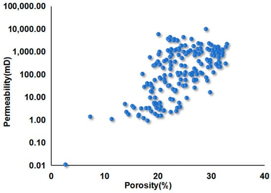
Figure 2.
Porosity and permeability of the reservoir.
2.2. Logging Response Characteristics
It is explained in the interpretation conclusion of Figure 3 that all black intervals represent oil layers. In contrast, black intervals with numbers represent water-flooded layers, where number 1 denotes strongly water-flooded layers, number 2 denotes moderately water-flooded layers, and number 3 denotes weakly water-flooded layers. As shown in Figure 3, the gamma ray curves of water-flooded layers all show a decreasing trend, indicating that after oil layers are flooded, some radioactive substances can be carried away, decreasing the curve values. In the resistivity curve, with the increase of water saturation, injected water displaces oil along the large pores of the reservoir. It dissolves reservoir salts, resulting in a specific decrease in resistivity. The resistivity of oil layers is greater than 8 Ω·m; that of strongly water-flooded layers ranges from 2 to 5 Ω·m, moderately water-flooded layers range from 4 to 6 Ω·m, and weakly water-flooded layers range from 10 to 16 Ω·m, which has little difference from the resistivity of oil layers.
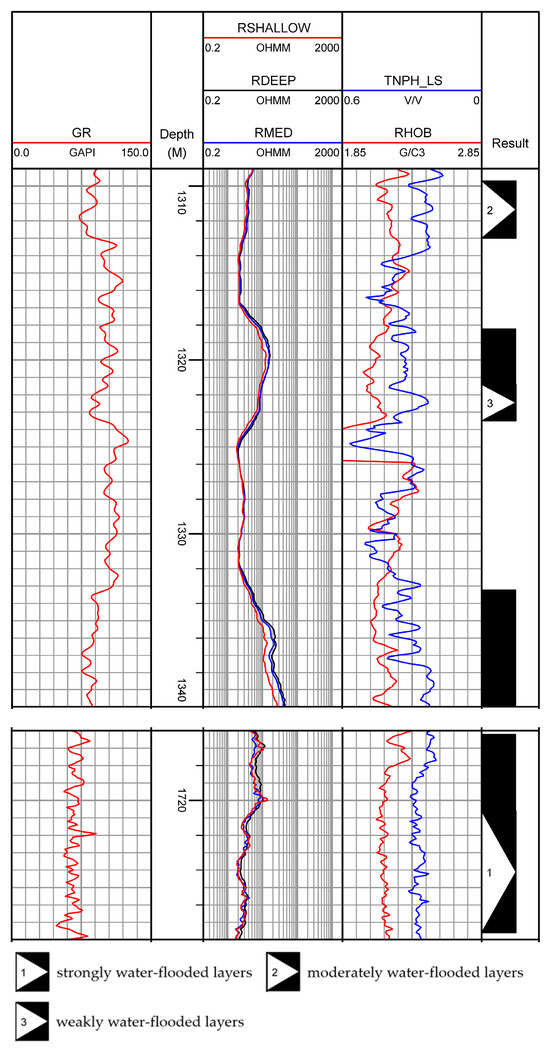
Figure 3.
Logging Response Characteristics.
The distributions of oil, water-flooded, and water layers overlap on various logging curves. The variation range of compensated neutron logging responses of water-flooded layers is similar to that of oil layers, so effective differentiation between water-flooded layers and oil layers cannot be achieved through the compensated neutron curve.
In the study block, the variation ranges of density and compensated neutron logging responses between water-flooded layers and oil layers are highly similar, and the resistivity of weakly water-flooded layers is little different from that of oil layers. Therefore, it is difficult to accurately distinguish oil and water-flooded layers at different levels relying solely on logging response characteristics.
2.3. Reduced Applicability of the Archie Formula After Reservoir Water Flooding and Its Causes
The Archie equation is a quantitative model establishing the relationship between resistivity and oil saturation, which is developed based on pure sandstone reservoirs [2,3]. Its expression is as follows:
where, is the oil saturation, is the cementation exponent, a is the lithology coefficient, n is the saturation exponent, is the formation water resistivity, is the original formation resistivity, and is the porosity. Therefore, the application of the Archie equation requires three prerequisites: the reservoir is pure sandstone with low mineral content and no additional conductive effect; the fluid in the pores is oil-water two-phase and uniformly distributed, with homogeneous reservoir properties; the reservoir cementation state is stable, and water injection development does not change the pore structure of lithology.
Water flooding of oil layers disrupts the physical and chemical equilibrium of the original reservoir [2,3], fundamentally undermining the application basis of the Archie equation, and its applicability varies significantly across different water flooding stages. No significant changes occur in lithology and pore structure of weakly water-flooded layers, with slight clay mineral swelling and minor influence of additional conductivity. However, in moderately and strongly water-flooded layers, its applicability decreases significantly with a sharp increase in errors. This is attributed to the gradually enhanced influence of additional conductive responses: water injection causes swelling of clay minerals (montmorillonite, illite) and forms a conductive network of clay-bound water, resulting in measured resistivity lower than the theoretical resistivity of pure sandstone. The heterogeneity of pore structure is intensified: long-term water injection scouring leads to cement dissolution and deteriorated particle sorting, forming a microstructure with macropores and microvoids, which is inconsistent with the uniform pore type assumed by the Archie equation. In addition, the heterogeneity of fluid distribution is enhanced, with residual oil filling the pores non-uniformly.
The Archie equation assumes the reservoir is pure sandstone, where only formation water conducts electricity without additional conductive components. However, during water flooding, the swelling of clay minerals creates an additional conductive network, directly violating this assumption. In the moderate to strong water flooding stage, injected water undergoes ion exchange and hydration with clay minerals in the reservoir. Montmorillonite can adsorb water molecules, causing the crystal layer spacing to expand from the dry to the wet state, with a volume expansion rate of over 30%. Although illite has weaker expansibility, it adsorbs water molecules through surface charges to form a water film, resulting in a volume expansion rate of approximately 5% to 15%. The swollen clay minerals fill some pores, and at the same time, the exchangeable cations (such as Na+, Ca2+) on their surfaces form conductive paths with ions in the injected water, known as the clay-bound water conductive network.
The Archie equation also assumes that the reservoir has a single pore type, uniform distribution dominated by intergranular pores, and slight differences in pore size. Nevertheless, long-term water flooding scouring in the moderate to strong water flooding stage reconstructs the pore structure, forming a heterogeneous system with both macropores and micropores. The long-term scouring of injected water dissolves cements (such as calcite and dolomite) in the reservoir. The dissolution rate of cements is about 5% to 15% in moderate water flooding and can reach 15% to 30% in strong water flooding. After cement dissolution, the original small pores expand into macropores, and the particle sorting deteriorates (the sorting coefficient increases from 1.2–1.5 to 1.8–2.2), forming a structure where macropore channels and micropore retention zones coexist.
Additionally, the Archie equation assumes a stable reservoir cementation state (the cementation exponent m is usually set to 2.0). However, cement dissolution and particle reorganization in the moderate to strong water flooding stage cause changes in the m value, undermining the equation’s parameter stability. As shown in Figure 4, in the moderate water flooding stage, the amount of cement dissolution is small, and there is still a certain cementation force between particles. Hence, the m value decreases from 1.9–2.0 to 1.7–1.8. In the strong water flooding stage, a large amount of cement dissolves, the supporting force between particles weakens, some particles migrate, and the m value further decreases to 1.5–1.6, even showing local looseness.
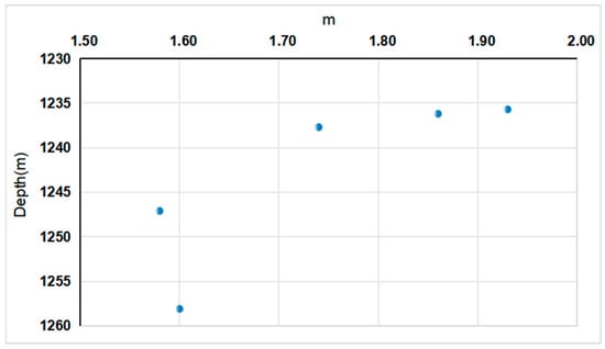
Figure 4.
The variation in the cementation exponent (m).
According to industry standards, the Archie equation fails to accurately identify water-flooded zones when geological changes reach the following comprehensive thresholds: the clay volume fraction exceeds 10%, the montmorillonite expansion rate exceeds 40%, the porosity standard deviation exceeds 3.5%, the cement dissolution rate exceeds 15%, and the fluctuation range of the cementation exponent exceeds 10%.
2.4. Histogram Gradient Boosting Classifier (HistGBDT)
Identifying water-flooded layers is a multivariate mapping problem involving reservoir physical properties, fluid characteristics, and logging responses. However, traditional methods rely on linear formulas (such as the Archie equation) or empirical statistical models, which struggle to handle the complex correlations caused by reservoir heterogeneity. In addition, the coring recovery rate of water-flooded layers is low, and the core integrity is poor. After water flooding, reservoir cements (e.g., clay minerals) swell upon contact with water and their strength decreases, making wellbore walls prone to collapse during coring, resulting in broken and missing cores. Limited by the size of coring tools, missed coring or layer mixing is likely to occur in water-flooded layers with a thickness of less than 0.5 m. Moreover, preserving core fluids is difficult, which easily affects the accuracy of the analysis. The imbalance between wellbore pressure and reservoir pressure during coring leads to the volatilization of light components of crude oil and the overflow of formation water in cores, failing to reflect the original oil-water saturation accurately. Clay mineral (montmorillonite, illite) swelling caused by water flooding further damages the pore structure, resulting in significant deviations between physical parameters such as core porosity and permeability and the original underground state. Therefore, the accuracy of water-flooded layer identification methods combining traditional Archie or statistical models with core data is challenging to improve.
Machine learning integrates multivariate data to automatically mine high-order nonlinear relationships between parameters and capture implicit correlations between logging curves and water-flooding levels, thus being widely applied in water-flooded layer identification methods [2,3,4,5]. It solves key problems such as scarce coring data of water-flooded layers, easy distortion of core fluids, and poor adaptability to heterogeneous reservoirs, while reducing production costs and improving analysis efficiency. Machine learning methods reduce the reliance on coring for special reservoirs, and can capture key information of thin layers to realise automatic identification of fine-level categories.
Machine learning has been widely used in the research of water-flooded layer identification. The core advantage of Random Forest lies in its feature screening and anti-overfitting capabilities, making it suitable for integrating multi-source heterogeneous data for water-flooding level classification [6,7,8]. Gradient boosting decision trees (XGBoost/LightGBM) focus on high-precision fitting of small-sample data and improve model performance by iteratively optimizing residuals, which is one of the core technologies for reducing coring costs. Back Propagation Neural Network (BPNN) excels at processing nonlinear mapping relationships and can integrate geological, seismic, and logging data to identify residual oil enrichment patterns [9]. Support Vector Machine (SVM) transforms low-dimensional nonlinear problems into high-dimensional linearly separable problems through kernel function transformation. It applies to water-flooded layer identification in thin and low-resistivity reservoirs [4,9].
Among the ensemble learning methods of traditional machine learning, gradient boosting decision trees (XGBoost/LightGBM) have demonstrated advantages in small-sample fitting and efficiency [4,9,10]. As an optimized evolution direction, Histogram-based Gradient Boosting Classifier (HistGBDT) is more suitable for the core needs of water-flooded layer identification scenarios. By mapping continuous features into histograms for split decision-making, it not only significantly reduces computational complexity and memory usage (with efficiency improved by more than 30% compared with XGBoost), perfectly solving the time-consuming problem in multi-parameter integration, but also the discretization of histograms naturally enhances the model’s robustness to noisy data. In fragmented data scenarios such as high-water-cut unconsolidated reservoirs, its anti-overfitting capability is superior to ordinary gradient boosting decision trees, enabling more accurate screening of key features such as the ratio of deep to medium lateral resistivity. In addition, its efficient utilization of small-sample data can further reduce reliance on core calibration data. HistGBDT is expected to achieve higher-precision water-flooding level classification in reservoirs with high porosity, high permeability, firm heterogeneity, and thin layers where coring data is scarce, thus being applied in water-flooded layer identification practice.
HistGBDT is an optimized version of Gradient Boosting Classifier (GBDT). It solves the problems of slow training speed and high memory usage of traditional GBDT in large-data scenarios, and is one of the core algorithms for classification tasks. GBDT is an ensemble learning algorithm that builds a strong classifier by serially training weak classifiers (decision trees) and gradually correcting errors. Its core logic is to use a simple constant as the initial prediction value, where the model error is significant. Weak classifiers are trained iteratively: one decision tree is trained each time, aiming to fit the error gradient of the previous round of the model (the direction of difference between the current predicted value and the actual label), which is equivalent to using the new decision tree to correct the errors of the previous round. All trees are weighted and integrated, and the prediction results of each tree are accumulated according to the weight (learning rate, which controls the contribution of a single tree), and finally, the prediction result of the strong classifier is obtained [4,9,10]. As shown in Figure 5a, the problem of traditional GBDT lies in the need to calculate the split gain (to determine whether to split the decision tree at this point) for each feature value. When the feature is a continuous value or the data volume is extremely large (such as logging curves), the training speed becomes slow, as all possible values of the feature need to be traversed, and the time complexity increases linearly with the data volume. Meanwhile, the memory usage is high, as all original values of the feature need to be stored, which easily leads to memory overflow in large-data scenarios.
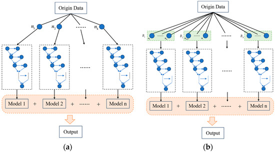
Figure 5.
Schematic diagram of GBDT and HistGBDT algorithms. (a) GBDT; (b) HistGBDT.
As shown in Figure 5b, HistGBDT no longer retains the original values for each continuous feature but divides them into multiple intervals (bins) [11]. For example, the gamma ray curve is divided into intervals such as [<50, 50–60, …, 100+]. It then counts the number of samples, error gradient, and sum of squared error gradients (the core indicators for calculating split gain) within each interval to form a histogram. Binning converts the infinite possible values of continuous features into limited intervals, which can significantly reduce the amount of computation.
Traditional GBDT needs to traverse each original value of the feature to calculate the split gain and determine whether the error decreases after splitting. In contrast, HistGBDT only needs to traverse each interval boundary. For the histogram of each feature, an attempt is made to split at each interval boundary. For instance, GR is split at 80 into [0–80, 81+], the error reduction (gain) after splitting is calculated, and the split point with the maximum gain is selected.
The core mathematical principle of HistGBDT is consistent with that of the traditional GBDT, both based on the additive model and gradient descent framework. Its innovation lies in optimizing the feature split calculation with histograms rather than changing the core mathematical logic.
HistGBDT follows the general paradigm of gradient boosting, constructing a strong classifier by iteratively training weak classifiers (decision trees) and accumulating their results. The core formulas are as follows:
The model is composed of weighted accumulation of decision trees. Where is the predicted value of sample x, denotes the -th decision tree, represents the learning rate of the -th tree, and is the number of decision trees.
where is the number of samples, and is the true label of sample . Gradient boosting adopts a greedy strategy for iterative optimization, using a constant function as the initial model.
Calculate the negative gradient :
Train the -th decision tree to fit the negative gradient, and update the model.
where is optimized through line search.
The core of training a single decision tree is to find the optimal split point, which minimizes the loss of the left and right child nodes after splitting. For a certain value of feature , the change in loss after splitting is measured by information gain. For the current node S, its loss is
where is the predicted value of node S.
Feature is split at value into left child node and right child node , with the split gain being:
The innovation of HistGBDT lies in compressing feature values using histograms (binning) to reduce the computation of split points. Its mathematical essence is to use interval statistics instead of individual sample calculations. For a continuous feature , its value range is divided into b non-overlapping intervals (bins).
where represents the -th bin (interval), which is a left-closed and right-open interval. denotes the left boundary included in this interval, and denotes the right boundary not included in this interval. This left-closed and right-open interval division method is common in feature binning. The intervals are non-overlapping, ensuring that each feature value can be uniquely assigned to one bin and all values are covered. Subsequent statistical calculations based on binning will not have the problem of duplicate or missing statistics.
where represents the number of samples, denotes the sum of gradients, and stands for the sum of squared gradients. Traditional methods need to traverse all values of feature , while HistGBDT only needs to traverse bin boundaries. For bins , assuming splitting between and , the left child node contains to , and the right child node contains to , then the statistics of the left child node are as follows:
Then the statistics of the right child node are as follows:
where , and are the total statistics of the current node. Taking squared loss as an example, the node loss can be expressed as
Then the split gain is
By traversing all bin boundaries to find the split point corresponding to the maximum , the computational complexity is reduced from O(k) (where k is the number of feature values) to O(b) (where b is the number of bins). The more detailed mathematical derivations of HistGBDT are described in Supplementary Materials: Equations (S1)–(S11).
2.5. Data Preprocessing
In the preprocessing stage of the HistGBDT model training, missing values in the dataset are identified using descriptive statistical methods, and the missing proportion of each feature is calculated. Targeted handling strategies are adopted based on differences in feature types and missing rates.
For missing values in a numerical feature (such as GR, RDEEP, etc.), the K-nearest neighbor imputation method (with K set to 5) is used for filling. This method finds the five nearest neighbor samples most similar to those with missing values. It fills the missing items using the mean value of their features, with distances calculated using Euclidean distance.
where represents the Euclidean distance between the target sample and the complete sample ; denotes the index of the feature with missing values in the sample; stands for the j-th feature value of the target sample ; and is the j-th feature value of the complete sample . Subsequently, K-nearest neighbors are selected.
Among them, refers to the samples corresponding to the first five distances obtained by sorting the distances between all samples in the complete sample set and the target sample in ascending order. For missing value imputation,
Here, denotes the imputed value for the missing value in the -th feature of the target sample, and represents the -th feature value of the -th nearest neighbor sample.
The processing of noisy data mainly involves two steps: detection and correction. The z-score analysis method is applied for detection. The Z-score of data points (representing the standardized deviation degree) is calculated for each numerical feature, with the threshold set to 3. Specifically, data points with a deviation from the mean greater than three are identified as outliers and classified as noise.
Here, represents the Z-score of the -th sample in the -th numerical feature, reflecting the deviation degree of the feature value of this sample from the overall distribution; is the original value of the -th sample in the -th numerical feature; denotes the mean value of the -th numerical feature; and stands for the standard deviation of the -th numerical feature.
Linear interpolation is used to correct the detected random noise. Based on the two valid samples adjacent to the outlier (one before and one after), the missing normal values are calculated through linear fitting to ensure the continuity of the data sequence.
Here, denotes the interpolated result of the noisy data; represents the feature value of the preceding valid sample, and stands for the feature value of the subsequent valid sample; is the position of the noisy data, is the position of the preceding valid sample, and is the position of the subsequent valid sample.
2.6. Model Optimization Strategy Based on HistGBDT
In oil and gas exploration and development, fluid type identification based on logging curves is a core link in reservoir evaluation. HistGBDT is widely applied in this task due to its strong ability to fit high-dimensional data and its robustness to missing values. However, the fixed parameter configuration of the basic model is often complicated when adapting to the complex distribution of logging data, which easily leads to underfitting or overfitting problems. This paper conducts optimization research to address the limitations of the basic model by constructing a parameter optimization model, clarifying the optimization strategy, and verifying its effectiveness.
The parameter configuration of the basic model has intense subjectivity. Core parameters such as the number of iterations and tree depth are preset based on manual experience, without considering the specific distribution characteristics of logging data, such as unbalanced fluid type samples and differences in feature correlation. This may result in overfitting to data or underfitting to complex data, leading to insufficient model adaptability. Meanwhile, the basic model only evaluates performance through a single split of the training and test sets, lacking a cross-validation link. It is thus challenging to eliminate the impact of randomness in data splitting on the results, and the generalization ability of the basic model is weak. In addition, the performance of gradient boosting models depends on the collaborative optimization of hyperparameters. Fixed parameters cannot achieve the optimal combination, which limits the upper limit of model performance.
As shown in Table 1, combining the algorithm characteristics of HistGBDT and the features of logging data, four core hyperparameters that have the most significant impact on model performance are selected to construct a search grid, covering the key regulatory dimensions of underfitting and overfitting. By adjusting the number of iterations, the number of weak learners is regulated to balance the fitting ability and computational cost; by adjusting the tree depth, the model complexity is regulated to enhance the fitting ability; by adjusting the learning rate, the contribution weight of a single tree is regulated-a small learning rate requires more iterations and has stronger stability; by adjusting the minimum number of samples in leaf nodes, the purity of leaf nodes is regulated-a large number of samples can suppress overfitting. The parameter grid contains a total of 36 combinations (2 × 3 × 3 × 2), which can fully cover potential optimal configurations. Through grid search, the parameter combination with the highest cross-validation accuracy is finally selected as the final configuration of the optimized model.

Table 1.
The differences of parameter configuration.
The optimized model constructs a dual verification system of cross-validation optimization and test set evaluation. In the parameter optimization stage, 3-fold cross-validation is used to evaluate the generalization ability of each parameter combination, ensuring that the selected parameter combination performs stably on different data subsets; in the performance evaluation stage, after fitting the optimal parameter combination to the complete training set, the final performance is evaluated on an independent test set, forming a direct comparison with the test set results of the basic model. Compared with the single split evaluation of the basic model, this logic can better eliminate the interference of data randomness and improve the credibility of the performance evaluation.
3. Results and Discussions
3.1. Data Features
In the case of lacking core data and having limited logging data, a total of 6 logging curves, including GR, RDEEP, RMED, RSHALLOW, TNPH, and RHOB, were selected.
Figure 6 shows the correlation coefficient matrix of the six selected logging curves (GR, RDEEP, RMED, RSHALLOW, TNPH, RHOB), which intuitively presents the degree of linear correlation between the curves. Among them, the three types of lateral resistivity curves (RDEEP, RMED, RSHALLOW) exhibit a strong positive correlation (correlation coefficient: 0.88–0.97), reflecting their commonality in characterising reservoir fluid properties. The correlation coefficients between GR, TNPH, RHOB and various resistivity curves are all close to 0, indicating no significant linear correlation. This reveals a lack of direct linear connection between reservoir physical property indicators and fluid sensitivity indicators. However, the Archie formula relies on the linear relationship between resistivity and porosity, thus leading to low applicability of the Archie formula in the study area. This matrix not only uncovers the reason why a single logging curve and linear model are difficult to distinguish between oil layers and water-flooded layers, but also provides data support for feature selection and integration of the subsequent HistGBDT model.
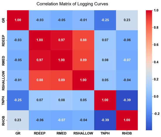
Figure 6.
Correlation matrix of logging curves.
The dataset used in this study was collected from three wells and consists of 4375 sample depth points, six numerical features, and one target variable. The sample distribution is illustrated in Figure 7. Where, Water represents water layers, WF1 represents strong water-flooded layers, WF2 represents moderate water-flooded layers, WF3 represents weak water-flooded layers, and OIL represents oil layers. The figure clearly shows the proportional differences of various fluid types at the logging data depth points selected in the study, providing a fundamental sample distribution basis for subsequent research work, such as analyzing different fluid types and constructing water-flooded layer identification models.
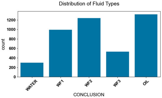
Figure 7.
Distribution of fluid types.
Figure 8 shows the feature distribution map classified by fluid type. Multiple subgraphs are used to respectively display the distribution characteristics of the six key logging curves (GR, RDEEP, RMED, RSHALLOW, TNPH, RHOB) under different fluid types. It can be observed from the figure that there are distribution differences and overlaps in various logging curve indicators between oil layers, fluid types related to different water-flooding levels, and water layers. Among them, the distribution ranges of water-flooded layers and oil layers in indicators such as RHOB and TNPH are highly similar, and there is also an inevitable overlap between weak water-flooded layers and oil layers in resistivity curves. This reflects that it is difficult to accurately distinguish oil layers from water-flooded layers of different levels relying solely on a single logging curve.
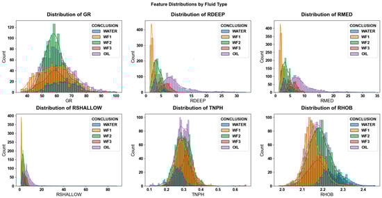
Figure 8.
Feature distributions by fluid type.
3.2. Model Performance
As shown in Table 2, from the perspective of model fitting effect and error control, all key indicators corresponding to a TEST proportion of 0.1 are at the optimal level: its coefficient of determination (R2) is 0.84, the highest among all proportions, indicating that the model has the strongest explanatory power for the training set data under this proportion and can better capture the correlation between logging curves and water-flooding levels. Meanwhile, its mean absolute error (MAE = 0.25) and mean squared error (MSE = 0.36). Root mean squared error (RMSE = 0.60) is the lowest among the four proportions, which means the deviation between the model’s predicted values and the actual values is the smallest, and the error control ability is optimal. This indicates that the model has the highest accuracy when the ratio of the training set to the test set is 9:1.
Table 2.
The effects under different test set proportions.
Figure 9 presents the evaluation results of the feature importance of logging curves by the basic HistGBDT model and the optimized HistGBDT model. In both models, RDEEP and RMED are key features. However, under the optimized model, the importance values of all features are generally higher, the gap in importance between RDEEP, RMED and other features is more significant, and the hierarchy of each feature’s importance is clearer. This indicates that the optimized model can identify key features more accurately, enhance the utilization efficiency of logging data, and thereby improve the discrimination performance of water-flooded layers.
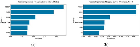
Figure 9.
Feature importance of logging curves. (a) Base Model; (b) Optimized Model.
Table 3 shows that the optimized model has achieved significant improvements in all core indicators: the accuracy rate exceeds 90%, the weighted F1-score has increased by 5%; among the regression indicators, R2 has risen by nearly 9%, and RMSE has decreased by approximately 29%. This indicates that the fitting degree between the predicted values and the true values of the optimized model has been dramatically enhanced.
Table 3.
Evaluation Index of the two models.
Analysis of Table 4 reveals that the optimized model has achieved particularly significant improvements in the identification ability of minority fluid types. Taking WF3 (with a sample proportion of approximately 12%) as an example, the recall rate of the basic model for WF3 is only 0.72, resulting in a large number of missed judgments. By adjusting the contribution weight of individual decision trees, the optimized model has enhanced its learning ability for minority samples: the recall rate of WF3 has increased to 0.88, and the number of missed judgments has decreased by more than 60%. This result verifies the improvement effect of parameter optimization on the sample imbalance problem and reflects the practical advantages of the optimized model.
Table 4.
Evaluation Index of the two models.
Figure 10 shows the confusion matrices of the two models. The proportion of diagonal elements (the number of correct classifications) has increased significantly. In the basic model, there were many cases where WF2 was misclassified into other categories and other categories were misclassified as WF2, and there was also a certain degree of cross-misclassification for WF3. In the optimized model, however, the number of cross-misclassifications, especially those related to WF2 and WF3, has decreased significantly (from 48 cases in the basic model to 15 cases) with clearer classification boundaries.
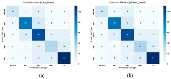
Figure 10.
Confusion matrix. (a) Base Model; (b) Optimzed Model.
The model was applied to the wells in the study area that did not participate in modeling. Table 5 shows model prediction examples, and Figure 10 is a comparison diagram of logging results. The last column presents the application effect diagram of the model, and the second-to-last column shows the original logging interpretation conclusions. Both Table 5 and Figure 11 reflect a high consistency between the discrimination results and the original interpretation conclusions, indicating that the model can accurately match the actual water-flooding conditions in well sections with drastic changes in resistivity curves and complex synergistic responses of porosity and density. This demonstrates its strong fitting ability for nonlinear correlations in logging data and excellent generalization performance.
Table 5.
Prediction examples.
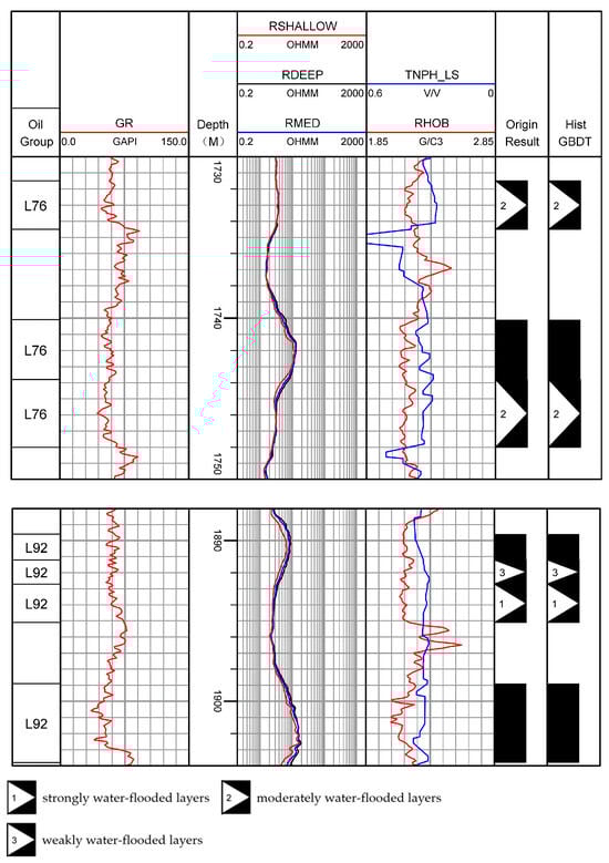
Figure 11.
Model illustration of the application of the PL-V well.
3.3. Comparison of Methods
As shown in Table 6, to verify the applicability and superiority of the HistGBDT adopted in this paper for the water-flooded layer identification task, this section conducts a multi-dimensional comparison between HistGBDT and traditional machine learning methods, namely BPNN and SVM. The demonstration focuses on prediction accuracy and model generalization performance, and the technical advantages of HistGBDT are verified by combining the characteristics of logging data and actual application requirements.
Table 6.
Evaluation Index of Three Models.
BPNN is a multi-layer feedforward neural network based on the error backpropagation algorithm. It realizes the fitting of nonlinear relationships through the connection of neurons in the input layer, hidden layer, and output layer. Its core logic is to calculate predicted values through forward propagation and correct weights through back propagation to minimize the loss function [2]. In water-flooded layer identification, it can integrate multi-source data such as geological, seismic, and logging data, and capture the complex mapping relationships between reservoir physical properties, fluid properties, and logging responses through the activation and interaction of multi-layer neurons. It is particularly suitable for processing multi-parameter data with strong nonlinear correlations.
SVM is a classification algorithm based on statistical learning theory. Its core principle is to map low-dimensional nonlinear problems to a high-dimensional linear space through kernel functions, and then find the optimal separating hyperplane to maximize the margin between samples of different categories [3]. In the field of water-flooded layer identification, relying on its advantages in small-sample learning and high-dimensional data processing capabilities, it is particularly suitable for water-flooded identification tasks of special reservoirs, such as thin layers and low-resistivity reservoirs. It can effectively process high-dimensional feature information in logging curves.
Significantly higher than those of BPNN and SVM, reflecting its stronger fitting ability for nonlinear correlations in logging data. In terms of generalization ability, HistGBDT achieves the highest generalization accuracy, and its cross-validation standard deviation is only 1/3 of that of BPNN and SVM, indicating that it has better stability in different data subsets and cross-block scenarios, with stronger resistance to data distribution shift. In terms of result interpretability, HistGBDT can clearly trace the identification logic through the visualization of feature importance and decision paths. In contrast, BPNN is a “black box” with no interpretability, and the kernel mapping process of SVM also lacks traceability. Thus, HistGBDT is more suitable for the engineering requirements of result credibility and logical verifiability in logging interpretation. Overall, HistGBDT is comprehensively superior to BPNN and SVM in terms of comprehensive performance, and is more adaptable to the water-flooded layer identification task of high-porosity, high-permeability and heterogeneous reservoirs.
As shown in Table 7, HistGBDT outperforms BPNN and SVM across all fluid clusters. HistGBDT boasts the highest accuracy rates (ranging from 0.88 to 0.96) and the fewest marginal errors, leading to the narrowest confidence intervals, which reflect its superior precision and stability. BPNN performs moderately, with lower accuracy and wider intervals than HistGBDT. SVM shows the poorest performance, having the lowest accuracy and the widest confidence intervals, indicating less reliability in classification.
Table 7.
Confidence Intervals of Three Models.
In Figure 12, the last three columns show the water-flooded layer identification result diagrams of the HistGBDT, BPNN, and SVM models, respectively. The identification results of HistGBDT are consistent with the original interpretation conclusions. In well sections with complex logging responses—especially those with drastic changes in resistivity curves and complex synergistic responses of porosity and density—it can more accurately match the actual water-flooding conditions, demonstrating its strong fitting ability for nonlinear correlations in logging data and excellent generalization performance. The identification results of BPNN and SVM have more obvious deviations from the original results, reflecting that traditional machine learning methods are affected by their own limitations in the water-flooded layer identification task: BPNN is prone to overfitting, while SVM has weak adaptability to multi-classification and complex data.
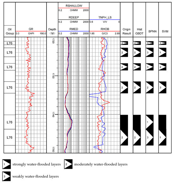
Figure 12.
An example of misjudgment between BPNN and SVM of PL-V well.
BPNN has significant limitations: it is highly dependent on network topology and parameter initialization, and easily falls into local minima; it has strict requirements for data normalization, requiring complex preprocessing such as normalization and missing value interpolation—otherwise, the imbalance of weight update will be caused by differences in feature dimensions; moreover, the model has a “black box” characteristic, and the output results cannot trace feature contributions, making it challenging to meet the engineering requirements for result interpretability in logging interpretation. Meanwhile, its generalization ability decreases significantly in scenarios with small samples or unbalanced data distribution.
SVM also has obvious shortcomings in the identification of complex reservoirs: it is essentially a binary classification algorithm, and needs to be extended through one-vs-one or one-vs-rest strategies for the identification of multi-type water-flooded layers (strongly water-flooded, moderately water-flooded, weakly water-flooded, etc.), which easily leads to class imbalance errors and low identification accuracy for minority samples; the selection of kernel functions and parameter adjustment rely on manual experience, and blind use of nonlinear kernels is prone to feature over-mapping, which instead reduces classification accuracy; it is prone to training stagnation in large-scale logging data. At the same time, the kernel function mapping process lacks physical meaning interpretation, which is inconsistent with the demand for traceability of identification logic in engineering practice.
For high-porosity and high-permeability heterogeneous reservoirs, the industry requirement for the accuracy of water-flooded zone identification in the medium-high water cut stage is 75–85%. When traditional methods (such as the Archie equation and cross-plot) are adopted, the accuracy is usually only 70–80%, and they are easily affected by pore structure alienation. The optimized HistGBDT model achieves an accuracy of 91.57%. From the perspective of field application, the model must simultaneously meet the requirements of the missed judgment rate of weak water-flooded zones being less than 15% and the misjudgment rate of strong water-flooded zones being less than 8%. The optimized model reduces the missed judgment rate to 13% and the misjudgment rate to 7%, fully meeting the practical needs of tapping the remaining oil potential.
3.4. Research Limitations and Future Directions
Although this study has realized the identification of conventional water-flooded scenarios based on the HistGBDT model, there are still limitations regarding technical depth and engineering adaptability. From the perspective of model optimization, the discrete parameter optimization of GridSearchCV is prone to missing the optimal combination, and the single input of original logging features fails to solve the problems of redundant interference and insufficient capture of deep correlations. At the data support level, the lack of micro-pore structure data makes it difficult for the model to adapt to the complex water-flooding mechanism of heterogeneous reservoirs. In contrast, the static data structure cannot respond to the dynamic evolution characteristics of water injection development. In engineering applications, the identification blind areas in thin layers and edge water intrusion zones, as well as the attenuation of generalization in cross-block migration, further restrict the on-site practical value of the model.
To address these limitations, the following suggestions are put forward: in terms of parameter optimization, replace GridSearchCV with Bayesian optimization, preset parameter constraint boundaries in combination with reservoir physical properties, and conduct dynamic optimization through a Gaussian process surrogate model to improve parameter adaptability; in terms of feature processing, preprocess raw data via wavelet denoising, generate derived features such as resistivity ratio and porosity-density coupling based on reservoir mechanisms, and screen core features to reduce redundancy; in terms of model structure, embed a reservoir physical constraint module, capture the correlation of reservoirs at different depths through a multi-scale feature fusion layer, and realize the simultaneous optimization of parameter efficiency, feature quality and reservoir correlation capture.
To ensure the cross-block fast generalization performance of the model, the following suggestions are proposed: take static logging data (GR, resistivity, etc.) as the foundation, superimpose dynamic production data (injection-production pressure, liquid production profile) and micro-pore structure data (nuclear magnetic logging, imaging logging) to achieve multi-source data alignment; for thin layers, extract curve shape features and dynamic production response fusion features to enhance thin-layer signals; for edge water zones, introduce dynamic derived features such as injection-production interference coefficient to characterize fluid boundaries; finally, transfer the model parameters of mature blocks to new blocks through transfer learning, and conduct in-depth analysis combined with block geological differences.
4. Conclusions
Taking the high-porosity, high-permeability, and strongly heterogeneous reservoirs of the Guantao Formation in the Penglai 19-3 Oilfield as the research object and aiming at the bottlenecks of traditional water-flooded layer identification methods, this study systematically carried out research on water-flooded layer identification based on the Histogram Gradient Boosting Classifier (HistGBDT). It clarified the applicability and technical value of different methods and pointed out the direction for subsequent research.
Firstly, it revealed the core problem, which is that the applicability of the Archie formula in water-flooded layer identification in the study area has significantly declined. The formula is based on the assumptions of pure sandstone, uniform pores, and stable cementation. However, in the moderate and strong water-flooding stages of the Penglai 19-3 Oilfield, water injection causes clay mineral swelling to form an additional conductive network, long-term scouring leads to cement dissolution and increased heterogeneity of pore structure, and the remaining oil distribution shows firm heterogeneity. These factors fundamentally undermine the application basis of the Archie formula. The formula only has particular applicability in weak water-flooded layers and cannot meet the needs of accurate identification in the complete water-flooding stage.
Comparisons between the basic HistGBDT model and the optimized HistGBDT model show that the optimized model has significant advantages. The basic model relies on manually preset parameters, lacks a cross-validation link, is easily affected by the randomness of data splitting, and has limited generalization ability. In contrast, the optimized model uses GridSearchCV to search for 36 parameter combinations, and combines 3-fold cross-validation with independent test set evaluation. It achieves comprehensive improvements in core indicators and effectively solves the problems of sample imbalance and parameter adaptation.
Comparing the HistGBDT model with traditional machine learning methods (BPNN and SVM), the model proposed in this study has higher practical value. In terms of prediction accuracy, the test accuracy of HistGBDT reaches 0.92, far exceeding that of BPNN and SVM. In terms of generalization ability, its generalization accuracy is 0.88, and the cross-validation standard deviation is only 0.01, which is 1/3 of that of BPNN and SVM, showing better stability. More importantly, HistGBDT can trace the identification logic through the visualization of feature importance and decision paths. At the same time, BPNN and SVM have “black box” characteristics and cannot meet the demand for result interpretability in engineering practice. In addition, BPNN is prone to falling into local minima and has strict requirements for data preprocessing, while SVM is prone to class imbalance errors in multi-classification scenarios. HistGBDT effectively avoids these defects and is more suitable for the identification task of complex reservoirs.
In summary, the constructed optimized HistGBDT model, based on six logging curves including GR and RDEEP, realizes the accurate identification of oil layers and water-flooded layers of different levels, providing a reliable technical means for remaining oil potential tapping in the high-water-cut stage of the Penglai 19-3 Oilfield. Future research can be deepened in the directions of precision, multi-dimensionality and scenarioization: at the model level, Bayesian optimization will replace grid search, and a three-level feature system (original, derived and screened) will be constructed; at the data level, micro-data such as nuclear magnetic resonance and imaging logging will be integrated with dynamic production time-series information; at the application level, special models will be developed for thin layers and edge water intrusion zones, transfer learning will be used to enhance cross-block generalization, and visualization tools will be adopted to strengthen result interpretability. This series of optimizations will promote the transformation of water-flooded layer identification from experience-driven to data-mechanism-engineering collaborative-driven, providing important technical references for the development of similar reservoirs in the Bohai Bay Basin.
Supplementary Materials
The following supporting information can be downloaded at: https://www.mdpi.com/article/10.3390/pr13103219/s1, Equations (S1)–(S11).
Author Contributions
Conceptualization, H.Z. and W.Y.; methodology, H.Z., W.Y. and Z.Z.; software, H.Z.; validation, X.N., C.Z. and Z.Z.; formal analysis, H.Z.; investigation, H.Z.; resources, Z.Z.; data curation, H.Z.; writing—original draft preparation, H.Z. and W.Y.; writing—review and editing, C.Z., H.L. and H.Z.; visualization, Z.Z. and H.L.; supervision, X.N.; project administration, Z.Z.; funding acquisition, X.N. All authors have read and agreed to the published version of the manuscript.
Funding
This work was supported by the National Natural Science Foundation of China (No. 42474159).
Data Availability Statement
Data associated with this research are available and can be obtained by contacting the corresponding authors.
Acknowledgments
We thank the reviewers, and the editors for their constructive comments and editing, which immensely helped improve the clarity of the original manuscript.
Conflicts of Interest
The authors declare no conflicts of interest.
Abbreviations
The following abbreviations are used in this manuscript:
| GBDT | Gradient Boosting Decision Tree |
| HistGBDT | Histogram-based Gradient Boosting Classifier |
| BPNN | Back Propagation Neural Network |
| SVM | Support Vector Machine |
| GR | Gamma Ray |
| RDEEP | Deep Lateral Resistivity |
| RMED | Medium Lateral Resistivity |
| RSHALLOW | Shallow Lateral Resistivity |
| TNPH | Neutron Porosity |
| RHOB | Bulk Density |
| R2 | Coefficient of Determination |
| MAE | Mean Absolute Error |
| MSE | Mean Squared Error |
| RMSE | Root Mean Squared Error |
| WF1 | Strong water-flooded layers |
| WF2 | Moderate water-flooded layers |
| WF3 | Weak water-flooded layers |
| GridSearchCV | Grid Search with Cross-Validation |
References
- Liu, Y.; Luo, X.; Kang, K.; Li, T.; Jiang, S.; Zhang, J.; Zhang, Z.; Li, Y. Permeability characterization and directional wells initial productivity prediction in the continental multilayer sandstone reservoirs: A case from Penglai 19-3 oil field, Bohai Bay Basin. Pet. Explor. Dev. 2017, 44, 97–104. [Google Scholar] [CrossRef]
- Song, J.; Zhang, H.; Guo, J.; Han, Z.; Guo, J.; Zhang, Z. A new method for identifying reservoir fluid properties based on well logging data: A case study from PL block of Bohai Bay Basin, North China. Open Geosci. 2024, 16, 20220716. [Google Scholar] [CrossRef]
- Wang, F.; Bian, H.; Zhao, L.; Yu, J.; Tan, C. Electrical responses and classification of complex water-flooded layers in carbonate reservoirs: A case study of Zananor Oilfield, Kazakhstan. Pet. Explor. Dev. 2020, 47, 1299–1306. [Google Scholar] [CrossRef]
- Jiang, Z.; Liu, Z.; Zhao, P.; Chen, Z.; Mao, Z. Evaluation of tight waterflooding reservoirs with complex wettability by NMR data: A case study from Chang 6 and 8 members, Ordos Basin, NW China. J. Pet. Sci. Eng. 2022, 213, 110436. [Google Scholar] [CrossRef]
- He, W.Y.; Wu, Y.D.; Feng, L.X.; Li, C.X.; Wan, J.B.; Ni, G.H. Research on the Mechanism of Complex Water-flooded Layers and Well Logging Evaluation Methods in the M Oilfield. Appl. Geophys. 2025, 22, 1–16. [Google Scholar] [CrossRef]
- Guo, J.; Yang, E.; Zhao, Y.; Fu, H.; Dong, C.; Du, Q.; Zheng, X.; Wang, Z.; Yang, B.; Zhu, J. A New Method for Optimizing Water-Flooding Strategies in Multi-Layer Sandstone Reservoirs. Energies 2024, 17, 1828. [Google Scholar] [CrossRef]
- Wang, F.; Yang, H.; Jiang, H.; Kang, X.; Hou, X.; Wang, T.; Zhou, B. Formation mechanism and location distribution of blockage during polymer flooding. J. Pet. Sci. Eng. 2020, 194, 107503. [Google Scholar] [CrossRef]
- He, X.; Xie, K.; Cao, W.; Lu, X.; Wang, X.; Huang, B.; Zhang, N.; Cui, D.; Hong, X.; Wang, Y.; et al. Effect of CO2-assisted surfactant/polymer flooding on enhanced oil recovery and its mechanism. Geoenergy Sci. Eng. 2025, 244, 213473. [Google Scholar] [CrossRef]
- Yang, T.; Tang, H.; Wang, M.; Guo, X.; Tang, H.; Shi, X.; Liu, J. Prediction of total gas content in low-resistance shale reservoirs via models fusion—Taking the Changning shale gas field in the Sichuan Basin as an example. Geoenergy Sci. Eng. 2024, 235, 212698. [Google Scholar] [CrossRef]
- Wang, Y.; Sun, Y.; Yang, S.; Wu, S.; Liu, H.; Tong, M.; Lyu, H. Saturation evaluation of microporous low resistivity carbonate oil pays in Rub Al Khali Basin in the Middle East. Pet. Explor. Dev. 2022, 49, 94–106. [Google Scholar] [CrossRef]
- Caesary, D.; Kim, J.; Jang, S.J.; Quach, N.; Park, C.; Kim, H.M.; Nam, M.J. Numerical modeling and evaluation of lab-scale CO2-injection experiments based on electrical resistivity measurements. J. Pet. Sci. Eng. 2022, 208, 109788. [Google Scholar] [CrossRef]
- Liu, R.; Zhang, L.; Wang, X.; Zhang, X.; Liu, X.; He, X.; Zhao, X.; Xiao, D.; Cao, Z. Application and Comparison of Machine Learning Methods for Mud Shale Petrographic Identification. Processes 2023, 11, 2042. [Google Scholar] [CrossRef]
- Ishigami, T.; Irikura, M.; Tsukahara, T. Machine Learning to Estimate the Mass-Diffusion Distance from a Point Source under Turbulent Conditions. Processes 2022, 10, 860. [Google Scholar] [CrossRef]
- Alatefi, S.; Abdel Azim, R.; Alkouh, A.; Hamada, G. Integration of Multiple Bayesian Optimized Machine Learning Techniques and Conventional Well Logs for Accurate Prediction of Porosity in Carbonate Reservoirs. Processes 2023, 11, 1339. [Google Scholar] [CrossRef]
- Yang, Z.; Li, H.; Wang, X.; Meng, H.; Xi, T.; Hou, Z. Source identification of mine water inrush based on GBDT-RS-SHAP. Environ. Earth Sci. 2025, 84, 114. [Google Scholar] [CrossRef]
- Gao, W.; Li, Z.; Chen, Q.; Jiang, W.; Feng, Y. Modelling and prediction of GNSS time series using GBDT, LSTM and SVM machine learning approaches. J. Geod. 2022, 96, 71. [Google Scholar] [CrossRef]
- Dong, X.; Guo, M.; Wang, S. GBDT-based multivariate structural stress data analysis for predicting the sinking speed of an open caisson foundation. Georisk-Assess. Manag. Risk Eng. Syst. Geohazards 2024, 18, 333–345. [Google Scholar] [CrossRef]
- Mehmani, A.; Kelly, S.; Torres-Verdin, C. Leveraging digital rock physics workflows in unconventional petrophysics: A review of opportunities, challenges, and benchmarking. J. Pet. Sci. Eng. 2020, 190, 107083. [Google Scholar] [CrossRef]
- Franc, J.; Guibert, R.; Horgue, P.; Debenest, G.; Plouraboue, F. Image-based effective medium approximation for fast permeability evaluation of porous media core samples. Comput. Geosci. 2021, 25, 105–117. [Google Scholar] [CrossRef]
- Cui, L.-K.; Sun, J.-M.; Yan, W.-C.; Dong, H.-M. Multi-scale and multi-component digital core construction and elastic property simulation. Appl. Geophys. 2020, 17, 26–36. [Google Scholar] [CrossRef]
- SoltaniMoghadam, S.; Ansari, A.; Etemadsaeed, L.; Tatar, M.; Mahmoodabadi, M. Earthquake location and magnitude estimation using seismic arrival times pattern and gradient boosted decision trees. Artif. Intell. Geosci. 2025, 6, 100149. [Google Scholar] [CrossRef]
- Chen, Y.; Luo, T.; Sun, G.; Zhu, W.; Liu, Q.; Liu, Y.; Jin, X.; Weng, N. A Comprehensive Ensemble Model for Marine Atmospheric Boundary-Layer Prediction in Meteorologically Sparse and Complex Regions: A Case Study in the South China Sea. Remote Sens. 2025, 17, 2046. [Google Scholar] [CrossRef]
- Anderson, C.J.; Heins, D.; Pelletier, K.C.; Knight, J.F. Using Voting-Based Ensemble Classifiers to Map Invasive Phragmites australis. Remote Sens. 2023, 15, 3511. [Google Scholar] [CrossRef]


Disclaimer/Publisher’s Note: The statements, opinions and data contained in all publications are solely those of the individual author(s) and contributor(s) and not of MDPI and/or the editor(s). MDPI and/or the editor(s) disclaim responsibility for any injury to people or property resulting from any ideas, methods, instructions or products referred to in the content. |
© 2025 by the authors. Licensee MDPI, Basel, Switzerland. This article is an open access article distributed under the terms and conditions of the Creative Commons Attribution (CC BY) license (https://creativecommons.org/licenses/by/4.0/).