Article

Discrete-Time Linear Quadratic Optimal Tracking Control of Piezoelectric Actuators Based on Hammerstein Model

1
College of Electronic Information Engineering, Changchun University, Changchun 130022, China
2
Department of Control Science & Engineering, Jilin University, Changchun 130012, China
*
Author to whom correspondence should be addressed.
Processes 2025, 13(10), 3212; https://doi.org/10.3390/pr13103212
Submission received: 29 August 2025 / Revised: 5 October 2025 / Accepted: 6 October 2025 / Published: 9 October 2025
(This article belongs to the Section Process Control and Monitoring)

Abstract

To address the issue of hysteresis nonlinearity adversely affecting the tracking accuracy of piezoelectric actuators, an improved particle swarm optimization (PSO) algorithm is proposed to improve the accuracy of hysteresis model parameter identification. Additionally, a discrete-time linear quadratic optimal tracking (DLQT) control strategy incorporating hysteresis compensation is developed to improve tracking performance. This study employs the Hammerstein model to characterize the nonlinear hysteresis behavior of piezoelectric actuators. Regarding parameter identification, the conventional PSO algorithm tends to suffer from premature convergence and being trapped in local optima. To address this, a cross-variation mechanism is introduced to enhance population diversity and improve global search ability. Furthermore, adaptive and dynamically adjustable inertia weights are designed based on evolutionary factors to balance exploration and exploitation, thereby enhancing convergence and identification accuracy. The inertia weights and learning factors are adaptively adjusted based on the evolutionary factor to balance local and global search capabilities and accelerate convergence. Benchmark function tests and model identification experiments demonstrate the improved algorithm’s superior convergence speed and accuracy. In terms of control strategy, a hysteresis compensator based on an asymmetric hysteresis model is designed to improve system linearity. To address the issues of incomplete hysteresis compensation and low tracking accuracy, a DLQT controller is developed based on hysteresis compensation. Hardware-in-the-loop tracking control experiments using single and composite frequency reference signals show that the relative error is below 3.3% in the no-load case and below 4.5% in the loaded case. Compared with the baseline method, the proposed control strategy achieves lower root-mean-square error and maximum steady-state error, demonstrating its effectiveness.

1. Introduction

Piezoelectric actuators exploit the piezoelectric effect of ceramic materials to generate nanoscale micro-displacements [1]. Compared with traditional motor-driven actuators, piezoelectric actuators offer advantages such as fast response, high precision, high resolution, and compact size [2,3]. These actuators are widely used in precision control applications, including deflection mirrors, biological micromanipulation, and 3D printing [4,5,6]. The hysteresis behavior of piezoelectric actuators is rate-dependent [7]; as shown in Figure 1, the output displacement is frequency-dependent on the input voltage signal. With increasing input frequency, the maximum displacement of the hysteresis loop decreases while the minimum displacement increases, indicating that the peak-to-peak displacement reduces as the frequency rises. The variation in arrow width in the locally enlarged view further illustrates that the hysteresis loop becomes wider with increasing frequency, implying enhanced nonlinearity. The inherent nonlinear hysteresis of piezoelectric ceramics degrades the control accuracy of actuators, thereby limiting their application scope and performance improvement.
To mitigate the impact of hysteresis nonlinearity on the control accuracy of piezoelectric actuators, it is essential to develop a mathematical model that accurately captures this nonlinearity. Relying on this model, an appropriate control method can be devised to enhance tracking accuracy [8]. Hysteresis nonlinear modeling approaches are generally categorized into modular and integral types. Modular models mainly include the Hammerstein and Wiener models [9,10], while integral models incorporate frequency-dependent parameters into rate-independent frameworks, such as the dynamic Preisach and dynamic Duhem models [11,12]. Integral models are generally difficult to invert, which hinders controller design and limits their practical applicability. The Bouc-Wen model describes hysteresis using a simple auxiliary nonlinear differential equation, making it easy to implement and its inverse model straightforward to compute, which facilitates subsequent controller design [13]. In this study, a Hammerstein model incorporating the Bouc-Wen model is employed to characterize the nonlinear behavior of the piezoelectric actuator.
Parameter identification methods for hysteresis nonlinear models can be broadly classified into classical and heuristic approaches. Classical identification algorithms include recursive least squares [14] and maximum likelihood estimation [15]. Classical identification algorithms have been well developed; however, as the degree of system nonlinearity and the number of parameters to be identified increase, their performance becomes inferior to heuristic identification methods [16]. Heuristic algorithms are inspired by biological evolution. Common heuristic algorithms include genetic algorithms, differential evolution, particle swarm optimization (PSO), grey wolf optimization, and ant colony optimization [17,18,19,20,21]. Unlike classical methods, these algorithms do not require gradient information or continuity, having advantages such as information exchange within the given space and insensitivity to initial values. Among these, PSO has been widely applied in parameter identification owing to its simple structure, rapid convergence, and efficient information utilization [22]. Standard PSO uses fixed inertia weights and learning factors, it lacks dynamic adaptability. Consequently, particles with high fitness may be discarded during itera-tions, reducing population diversity and heightening the probability of premature convergence to local optima [23]., e.g., Brown et al. applied PSO to identify the parameters of a pneumatic artificial muscle actuator model [24]. Zheng et al. employed an improved PSO algorithm to optimize the hip and knee parameters of a wearable robot [25]. Fang et al. proposed a hybrid PSO algorithm to optimize the controller parameters of a permanent magnet synchronous motor servo system [26]. Sun et al. introduced an enhanced PSO algorithm to optimize the hyperparameters of an LSTM network, enhancing the precision of wind power prediction [27]. Xiao et al. proposed a PSO algorithm integrated with Q-learning to optimize battery disassembly tasks, improving the efficiency of human–robot collaborative disassembly compared with other algorithms [28].
The mainstream control approach for piezoelectric actuators involves designing a hysteresis compensator based on a hysteresis model, followed by a closed-loop controller to further enhance accuracy and robustness. Yu et al. proposed a fractional-order sliding mode control strategy with an extended state observer for a hysteresis-compensated system [29]. Liu et al. designed a proportional-integral (PI) controller incorporating a trap-based hysteresis compensator [30]. Salah, M. et al. developed a Bouc-Wen-based hysteresis compensator and designed a robust feedback controller with an observer for the compensated system, achieving effective tracking even at high reference signal frequencies [31]. However, the controller design processes of the aforementioned methods are complex and difficult to implement, limiting their practical applicability. Currently, tracking controller design aims either to achieve asymptotic convergence of the tracking error or to pursue optimal tracking control that balances tracking accuracy and overall system performance [32]. In addition, piezoelectric actuators must ensure system stability while accurately tracking the reference displacement. The linear quadratic regulator (LQR) aims to compute an optimal control law that minimizes a quadratic cost function defined by the system states and control inputs, subject to the constraints of the state equations and control limits. This ensures the system transitions smoothly from the initial state to the desired state [33,34]. The discrete-time linear quadratic optimal tracking (DLQT) controller shares similar principles with LQR. The key difference lies in the inclusion of a feedforward term in DLQT, which allows the closed-loop output to follow the reference input, while the feedback term enhances system robustness [32].
In this paper, an improved PSO algorithm is proposed to address the issues of the standard PSO, namely its tendency to fall into local optima and its slow convergence. The algorithm’s capability to escape local minima is enhanced by a crossover–mutation mechanism, while evolutionary factors are introduced to adaptively adjust the inertia weight and learning factors, thereby improving both convergence speed and optimization accuracy. The improved PSO is then applied to identify the nonlinear hysteresis model of the piezoelectric actuator. Based on the identified asymmetric Bouc–Wen model, a hysteresis compensator is designed to improve the linearity of the system, and a DLQT controller is subsequently developed for the compensated system to further enhance tracking accuracy and robustness.
The effectiveness of the improved PSO algorithm is validated through basis function tests and model identification experiments. Furthermore, the proposed control strategy, which combines hysteresis compensation with DLQT control, is verified through hardware-in-the-loop tracking experiments under both loaded and unloaded conditions.

2. Model Identification with an Improved PSO Algorithm

2.1. Dual Strategy Improved PSO Algorithm

2.1.1. Principle of PSO Algorithm

The PSO algorithm is a population-based intelligent search technique proposed by Kennedy and Eberhart in 1995. Its principle is derived by the foraging behavior of bird flocks [35]. Shi et al. proposed an improved PSO algorithm by introducing an inertia weight into the traditional PSO framework [23]. Ratnaweera et al. further enhanced the algorithm by replacing the constant learning factors with linearly varying values [36]. Under these modifications, the velocity and position of the i-th particle are updated using the following equations:
V i ( t + 1 ) = ω V i ( t ) + c 1 r 1 ( P b e s t i ( t ) X i ( t ) ) + c 2 r 2 ( G b e s t ( t ) X i ( t ) )
X i ( t + 1 ) = X i ( t ) + V i ( t + 1 )
The following is an explanation of the variables in Equations (1) and (2). Pbesti(t) is the current optimal position of the individual, and Gbest(t) is the optimal position of the group. ω is the inertia weight, c1 and c2 are the learning factors. Their expressions are shown in Equations (3) and (4).
ω = ω max ( ω max ω min ) T × t
c 1 = c max ( c max c min ) × t T c 2 = c min + ( c max c min ) × t T
In Equation (3), ω is a linear variation, where T is the maximum number of iterations, t is the current iteration number, and the value change range is [ ω min ,   ω max ] . The value of ω will affect the algorithm’s global and local search capabilities. In Equation (4), c1 and c2 are learning factors, with c1 affecting local search capabilities and c2 affecting global search capabilities.

2.1.2. Convergent Cross-Mutations

In this section, a crossover-mutation mechanism from the genetic algorithm [37] is introduced into the PSO to enhance the diversity of the particle population during the iterative evolution process. This integration enables the algorithm to escape from local optima. The fitness function is assumed to be proportional to the objective function, and the fitness value is minimized accordingly. Let the fitness value of particle x(t, i) at the t-th iteration be denoted as fitness(x(t, i)), and the average fitness of all particles fitness_av(x).
The schematic diagram of crossover and mutation is shown in Figure 2. For example, by solving for the lowest fitness function value. During the t-th iteration, for a particle x(t, i) in the current population S whose fitness value is higher than the average fitness value of the population, a particle x(t, k) is randomly selected from the particles of population S. Subsequently, the crossover and mutation operation is performed on x(t, k) and x(t, i) in accordance with Equation (5) to generate a new particle x(t, l). In Equation (5), R 1 = r a n d ( 0 ,   1 ) 2 , R 2 = e N ( 0 , 1 ) , rand(0, 1) denotes a random number within the range of 0 to 1, while N(0, 1) represents a random number following the standard normal distribution.
x ( t ,   l ) = R 1 x ( t ,   i ) + R 2 x ( t ,   k ) R 1 + R 2  
The decision to retain the newly generated particle is based on its fitness value. For example, by solving for the lowest fitness function value. If the fitness value of the new particle is lower than that of the original particle, x(t, l) is retained and replaces x(t, i); otherwise, it is discarded.
Figure 2. Schematic diagram of the crossover mutation operation between particle x(t, k) and x(t, i) in the improved PSO algorithm. Different colors represent different particles involved in the crossover–mutation process.
Processes 13 03212 g002

2.1.3. Adaptive Inertia Weights and Learning Factors

To harmonize the global and local search performance of the algorithm, the concept of an evolution factor is first introduced to reflect the degree of evolution of each particle at the t-th iteration. Then, this evolution factor is used to improve both the inertia weight and learning factors, enabling them to adaptively adjust in a dynamic manner.
Let the current maximum and minimum fitness values among all particles be denoted as fitness_max(x) and fitness_min(x), respectively. Then, the evolution factor of particle i at the t-th iteration is defined as follows:
K ( t , i ) = f i t n e s s ( x ( t , i ) ) f i t n e s s _ min ( x ) f i t n e s s _ max ( x ) f i t n e s s _ min ( x )
K(t, i) takes values in the range [0, 1]. When fitness(x(t, i)) = fitness_min(x), the value of K(t, i) is 0, indicating that the current particle x(t, i) has the strongest level of evolution. When fitness(x(t, i)) = fitness_max(x), the value of K(t, i) is 1, indicating that the current particle x(t, i) has the weakest level of evolution.
Evolutionary factors are introduced into the inertia weight and learning factors to enable both to adaptively adjust. Change the inertial weight from a linear transformation with respect to the iteration number T in Equation (3) to a nonlinear sine transformation. The improved expressions for the inertia weight and learning factors are given as follows:
ω ( t , i ) = K ( t , i ) × ω max ( ω max ω min ) × sin π 2 × ( 1 t T )
c 1 = 2 + 0.5 × 1 K ( t , i ) 1 t / T c 2 = 2 0.5 × 1 K ( t , i ) 1 t / T

2.2. Benchmark Function Test Experiment

In this section, optimal value search experiments are conducted on a series of benchmark functions with diverse characteristics using the modified PSO algorithm, aiming to demonstrate its adaptability and effectiveness across different optimization problems [38].
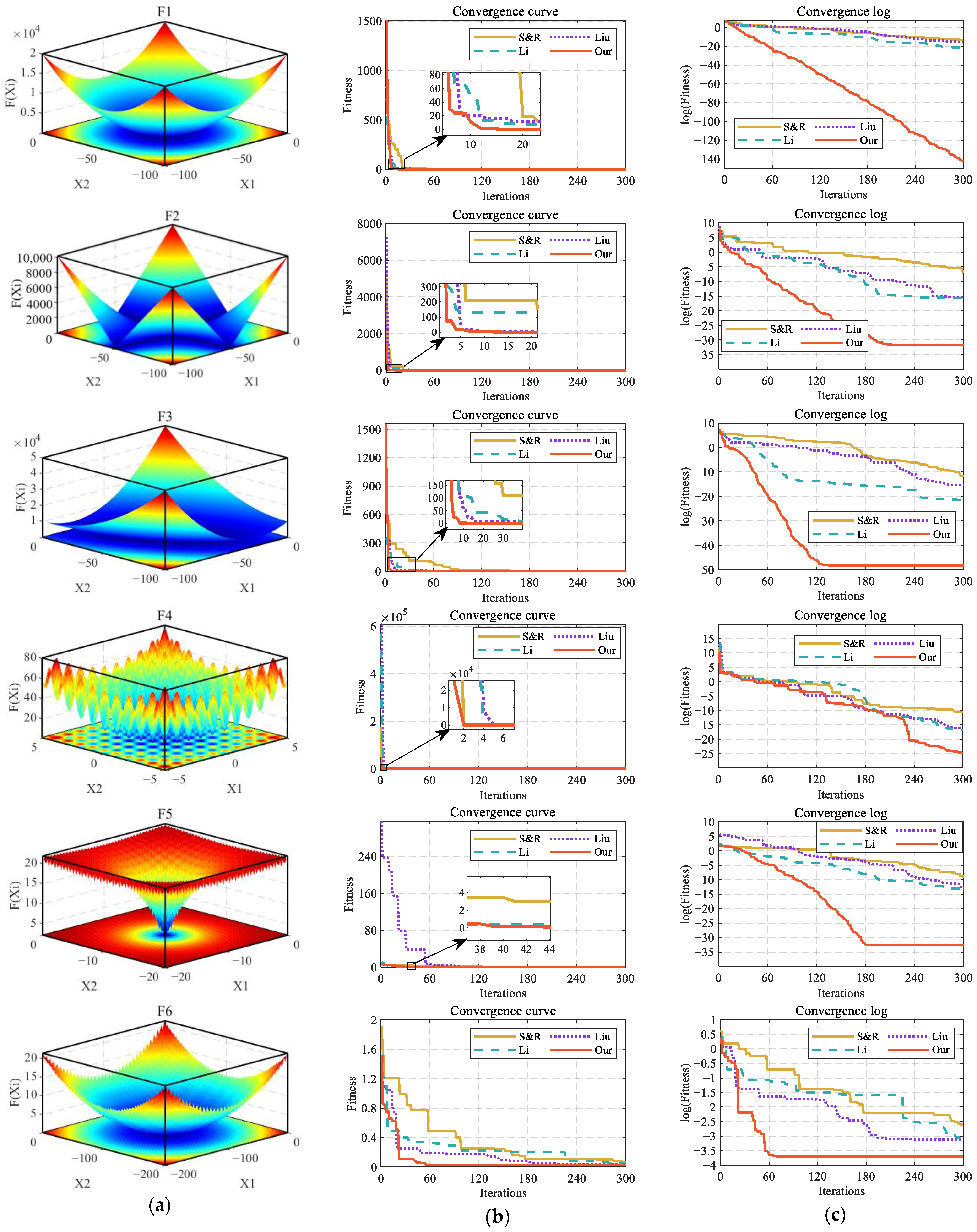
The three-dimensional plots of the benchmark functions are presented in Figure 3a. Functions F1–F3 are unimodal, characterized by a single global optimum without local optima, and are used to evaluate the algorithm’s convergence speed and accuracy. In contrast, Functions F4–F6 are multimodal, containing numerous local optima in addition to a global optimum, and are employed to assess the algorithm’s capability to escape local optima traps. For all six benchmark functions, the minimum value is 0.
Considering both practical requirements and computational complexity, the benchmark function test dimension is set to n = 5. The proposed modified PSO algorithm is employed to perform 20 independent optimizations on the benchmark functions and compared with the S&R-PSO [23,36], Liu-PSO [39], and Li-PSO [40]. The parameter settings for the benchmark function optimization tests of different PSO algorithms are summarized in Table 1. In this study, the key algorithm parameters were selected based on classical PSO design principles and empirical evidence reported in the literature [36]. The inertia weight ω decreases linearly from 0.9 to 0.4 to balance global exploration and local exploitation, while the learning factors c1 and c2 satisfy the condition c1 + c2 ≤ 4, which helps maintain stable convergence behavior. The population size S = 40 provides a trade-off between computational efficiency and search diversity, and the maximum iteration number T = 300 ensures stable convergence for improved PSO algorithms in benchmark function tests. This parameter configuration demonstrates satisfactory convergence speed and stability across multiple simulations, indicating that the chosen values are reasonable for achieving both optimization accuracy and computational efficiency.
Figure 3b illustrates the minimum value convergence curves obtained from 20 runs on different benchmark functions using various algorithms, while Figure 3c presents the convergence curves with optimization values plotted on a logarithmic scale.
The optimization results of the four algorithms on different benchmark functions are presented in Table 2. Best refers to the best fitness value obtained across 20 runs, Average indicates the mean fitness value, and Std represents the standard deviation.
For unimodal functions F1–F3 without local optima, the proposed improved PSO algorithm demonstrates significantly faster convergence and higher accuracy than the other three algorithms. For multimodal functions F4–F6 with multiple local optima, the overall performance of all four algorithms declines compared with the unimodal cases. Nevertheless, the proposed method still achieves superior results in terms of early convergence speed, final convergence accuracy, and stability (smaller standard deviations), thereby exhibiting stronger global search capability and robustness.
In addition to the comparative experiments presented in this study, it is also worth discussing the relationship between the proposed dual-improved PSO and other representative PSO variants. For example, chaotic PSO algorithm [41] enhances population diversity and mitigates premature convergence by introducing chaos mappings during the initialization or parameter update stages. Although such approaches can improve global search capability, their performance is often highly dependent on the specific chaotic map and control parameters, which makes it difficult to maintain consistent performance across different optimization problems. In contrast, the proposed dual-improvement PSO combines crossover–mutation mechanisms with adaptive adjustment of the inertia weight and learning factors, without relying on any specific mapping or parameterized design. This enables the algorithm to achieve better convergence speed and stability across various optimization scenarios.

2.3. Piezoelectric Actuator Model Identification

2.3.1. Experimental Platform and Model

Figure 4 illustrates the experimental platform. It includes the IPC-610L industrial control computer from Advantech (Beijing, China), the PCI-1710 data acquisition card, the Coremorrow E01 voltage control box, and the P11.X100S piezoelectric actuator platform.
The working principle diagram of the real-time control system of the experimental platform is shown in Figure 5. The industrial computer converts the digital control signals generated by the Simulink controller into analog signals through a data acquisition card and sends them to the voltage control box. The voltage control box generates voltage signals that meet the requirements to drive the piezoelectric actuator platform. After the piezoelectric platform generates displacement, its internal resistive position sensor detects the displacement signal in real-time and transmits it to the voltage control box. The voltage signal generated by the voltage control box is converted into a digital signal via the data acquisition card and returned to the Simulink controller of the industrial computer, where the controller calculates a new control signal based on the feedback signal and the reference signal, thus forming a closed-loop control.
In this paper, the static nonlinear component of the Hammerstein model for the piezoelectric actuators is formulated using an asymmetric Bouc-Wen model, while the dynamic linear component is described by a second-order linear system.
Considering the asymmetry of the hysteretic characteristics, the asymmetric Bouc–Wen model, as expressed in Equation (9), is employed to characterize the hysteresis behavior.
v = d u h h ˙ = α d u ˙ β u ˙ | h | sgn ( u ˙ h ) γ u ˙ + φ u ˙ sgn ( u )
In Equation (9), u and v represent the input and output of the hysteresis model, respectively. The variable h denotes the intermediate state of the hysteresis output. The parameter φ u ˙ sgn ( u ) is the asymmetric term introduced to capture the asymmetry of the hysteresis behavior (sgn is the sign function), and φ < 0 is the corresponding asymmetric factor. Parameters α and d control the size of the hysteresis loops, while β and γ govern the shape of the loops with respect to coefficients u ˙ and h .
The dynamic linear component must be capable of capturing the rate-dependent hysteresis behavior of the piezoelectric actuators [39]. In this study, the piezoelectric actuators are described as a mass-spring-damper system with hysteresis characteristics, and its dynamics are described by a second-order transfer function, expressed as:
G ( s ) = b s 2 + k 1 s + k 2
In Equation (10), b denotes the linear relationship between the output force F and the hysteresis input v. The parameters k1 = c/m, k2 = k/m, where c is the resistive coefficient, m is the mass of the piezoelectric actuators system, and k is the rigidity coefficient.

2.3.2. Model Identification and Validation

The hysteresis loop of the piezoelectric actuators exhibits minimal variation at low frequencies. Therefore, a 0.5 Hz sinusoidal signal is used as the excitation to collect input and output data from the experimental platform. The asymmetric Bouc-Wen model is identified using the improved PSO algorithm proposed in this paper, and comparisons are made with the improved PSO algorithms proposed by S&R [23,36], Liu [39], and Li [40]. The fitness function is defined as:
f i t n e s s ( x ) = 1 N i = 1 N ( X exp ( i ) X ( i ) ) 2
where Xexp(i) is the experimental output data and X(i) is the model output data recognised by the algorithm. N = 30,000, is the amount of experimental data. The smaller the fitness value, the better the fit.
Since the hysteresis model requires the identification of 5 parameters, which is the same as the problem dimension of the benchmark function test, the parameter settings of the PSO algorithm here are consistent with those in Table 1. The iteration curves of fitness function values for identifying the parameters of the asymmetric Bouc-Wen model using S&R-PSO, Liu-PSO, Li-PSO, and Our-PSO are shown in Figure 6.
All three algorithms demonstrate strong global search capabilities during the initial iteration phase and transition to local search around 20 generations. At this stage, the S&R algorithm exhibits the highest fitness value, Li’s algorithm ranks second, and the proposed method achieves the lowest fitness value. The introduction of the cross-variation mechanism enhances particle diversity, facilitating the generation of higher-quality particles. The proposed method completes local search by approximately 60 generations with the lowest fitness value, Li’s method converges around 150 generations, while the S&R method fails to complete local search and shows no convergence in fitness values. In summary, the improved PSO algorithm presented in this paper achieves accelerated convergence and improved accuracy.
The asymmetric Bouc-Wen hysteresis simulation model is constructed in MATLAB/Simulink (R2022b). Using the three sets of identification results, the model is excited by a 0.5 Hz sinusoidal signal. The system’s hysteresis loops are plotted as shown in Figure 7.
The red dotted line in Figure 7 represents the hysteresis loop identified by the improved PSO algorithm proposed in this paper. As shown in the zoomed-in section, compared with the other three improved PSO algorithms, the hysteresis model obtained by the proposed algorithm better fits the actual system. Table 3 summarizes the maximum fitting error (MMFE), root mean square error (RMSE), and relative error (RE) of the hysteresis models identified by the four algorithms—S&R-PSO, Liu-PSO, Li-PSO, and Our-PSO—relative to the reference hysteresis model.
Across all three evaluation metrics, the method proposed in this paper outperforms the other three comparative algorithms. Compared with the S&R, Liu, and Li algorithms, the proposed method reduced the MMFE by 18.5%, 16.7%, and 16.4%, respectively. The RMSE decreased by 16.8%, 13.7%, and 9.7%, while the RE dropped by 17.9%, 17.5%, and 15.4%, respectively. Although these reductions involve small numerical values, the accuracy of the hysteresis model critically determines the performance of subsequent hysteresis compensation. In scenarios where piezoelectric actuators operate at the micrometer or even nanometer scale, a high-precision hysteresis model facilitates more effective hysteresis compensation, thereby achieving more accurate system tracking.
To fully characterize the dynamic rate-dependent properties of the system, a set of sinusoidal sweep signals with linearly increasing frequencies (0.1–50 Hz) were used to excite the experimental platform equipped with the identified asymmetric Bouc-Wen model. The outputs of both the experimental platform and the model were recorded. The identification result of Equation (10) using MATLAB’s System Identification Toolbox is presented below.
G ( s ) = 3756000 s 2 + 1000 s + 3784000
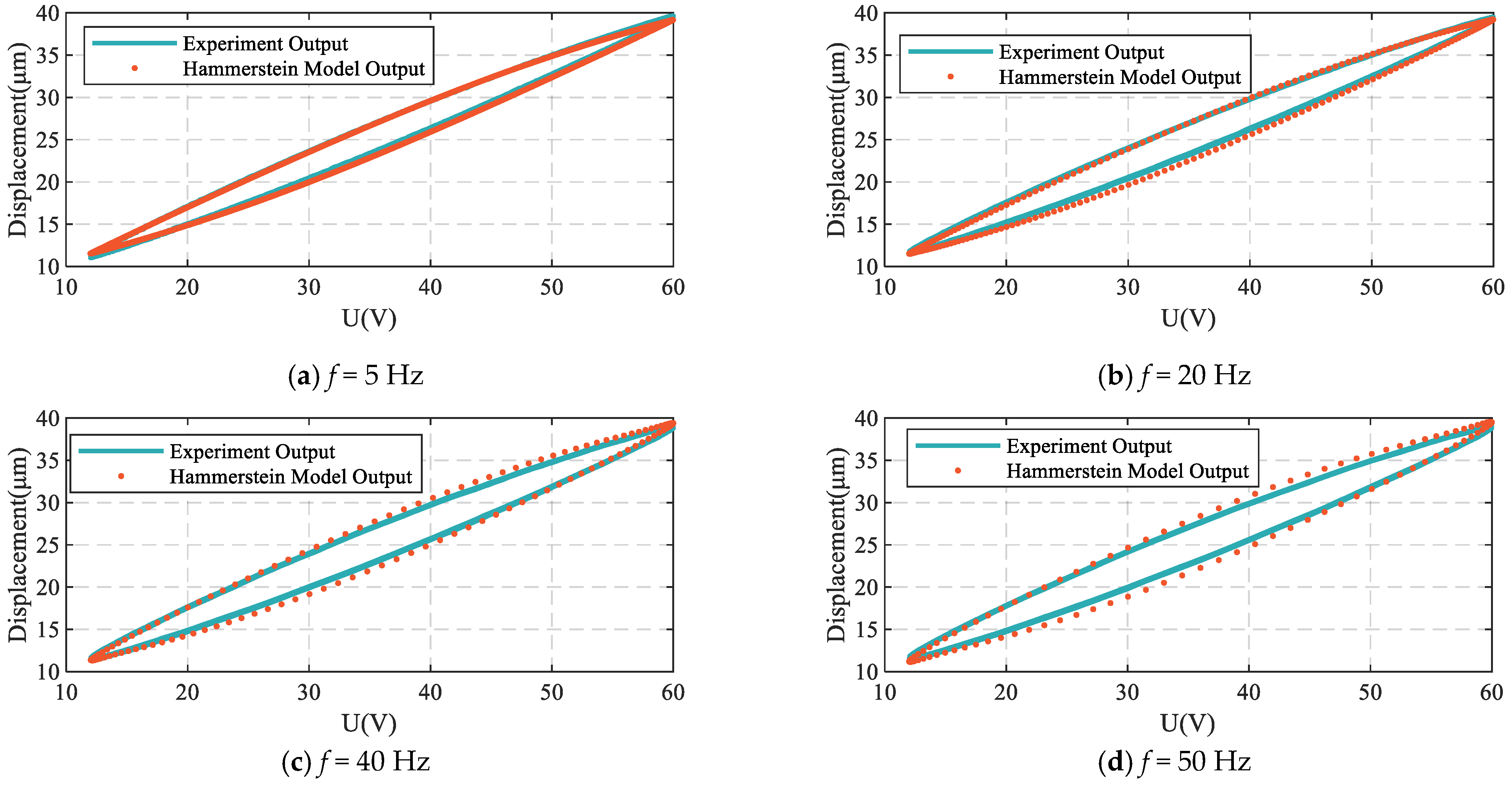
In order to evaluate the precision of the Hammerstein model, a simulation model was constructed in Simulink, and model fitting experiments were conducted. Both the experimental platform and the simulation model were excited with a voltage of u ( t ) = 12 ( 2 sin ( 2 π f t ) + 3 ) V , and frequencies f of 5 Hz, 20 Hz, 40 Hz, and 50 Hz were used, respectively. Hysteresis loop graphs were plotted according to the input and output signals of both the experimental platform and the model, as shown in Figure 8a–d. The modeling evaluation metrics are summarized in Table 4.
The model fitting experiments demonstrate that the Hammerstein model developed in this study can accurately represent the experimental platform. Across different input frequencies, the maximum fitting error is less than 1.2 μm, the root mean square error is below 0.7 μm, and the relative error remains under 3%.

3. Tracking Controller Design

In this section, a DLQT controller based on hysteresis compensation is designed to enhance the tracking control accuracy of the piezoelectric actuators. The piezoelectric actuators tracking control structure is illustrated in Figure 9.
The Bouc–Wen inverse model functions as a hysteresis compensator, connected in series at the input of the controlled plant to achieve approximate linearization. After hysteresis compensation, the system can be regarded as a second-order linear time-invariant system, which facilitates the design of the DLQT controller. The feedforward term of the DLQT controller, denoted as u1, enables the system output to track the reference signal, while the feedback term, u2, ensures the stability of the closed-loop system. Additionally, a Kalman Filter [42] (KF) is utilized to enhance state estimation for state feedback control.

3.1. Hysteresis Compensator

First, hysteresis compensator based on the Bouc–Wen model is designed and connected in series with the piezoelectric actuator to compensate for the system’s hysteresis nonlinearity. The hysteresis correction implemented through the inverse model is shown in Figure 10. Here, N−1 denotes the Bouc-Wen inverse model, and N represents the system’s hysteresis nonlinearity.
The hysteresis inverse model can be analytically expressed based on Equation (1) as:
u = 1 d ( v r + h )
The hysteresis compensator is designed based on the Bouc–Wen hysteresis model. Theoretically, after applying the inverse model N−1 and the hysteresis model N, the desired displacement vr equals the actual displacement v. It should be noted that the Bouc–Wen model employed in the compensator is rate-independent. As a result, the compensator effectively mitigates hysteresis nonlinearity at low and moderate input frequencies but its accuracy decreases as the excitation frequency increases. This limitation arises because the Bouc–Wen model does not explicitly account for rate-dependent effects. In practical applications, this implies that while the compensator significantly improves linearity under common operating conditions, its effectiveness may be reduced at high-frequency excitations, which needs to be considered when designing controllers for fast-response tasks.
Assuming negligible compensation errors and external disturbances, the compensated piezoelectric system can be equivalently described by the linear dynamic model in Equation (10). For controller design, Equation (10) is further expressed in discrete state-space form as follows:
x ( k + 1 ) = A x ( k ) + B v ( k ) y ( k ) = C x ( k )
In Equation (14), A and B represent the state transition matrix and input matrix, respectively, while C denotes the observation matrix. y is the output displacement of the piezoelectric actuators.

3.2. DLQT Controller Based on Hysteresis Compensation

When designing a tracking controller, both the system’s tracking errors and overall performance should be comprehensively considered. The linear quadratic regulator (LQR) defines the performance index as the quadratic integral of state and control variables in linear systems, aiming to optimise overall system performance. Mathematically, the objective of LQR is to determine the optimal control law under the constraints of state equations and control limits, such that the performance index based on system states is optimised, thereby guiding the system from the starting point to the target state.
This section focuses on the design of the DLQT controller for the system following hysteresis compensation, decomposing it into feedback and feedforward components. The feedback component employs state feedback control to stabilise the closed-loop system, providing robust performance and favourable dynamic characteristics. The feedforward component enables the closed-loop system output to accurately track the reference signal. By minimising a quadratic performance index, DLQT achieves asymptotic convergence of the tracking error while optimising overall system performance. The system tracking error can be represented as:
e ( k ) = r ( k ) y ( k )
in Equation (15), r(k) is the reference displacement; y(k) is the actual displacement.
Define the system performance metrics as:
J = k = 0 n 1 e ( k ) T Q e ( k ) + u ( k ) T R u ( k ) + e ( n ) T Q e ( n )
in Equation (16), n is a positive integer greater than 1 at the terminal moment. In the process of optimizing the objective function J, the values of matrices Q and R are crucial. Increasing the weight of Q can enhance the tracking control accuracy of the system but may result in higher energy consumption, while increasing the weight of R can reduce energy consumption but decrease tracking control accuracy. Therefore, a balance between control accuracy and energy consumption is required to achieve an optimal control scheme. strategy.
Based on the discrete-time linear quadratic tracking theory [32,43,44], the optimal tracking control law is derived by minimizing the performance metric in Equation (16) through solving the associated Riccati equation. The resulting control law is given as follows:
u ( k ) * = ( R + B T P B ) 1 B T g ( k + 1 ) ( R + B T P B ) 1 B T P A x ^ ( k ) u 1 = ( R + B T P B ) 1 B T g ( k + 1 ) u 2 = ( R + B T P B ) 1 B T P A x ^ ( k )
In Equation (17), x ^ ( k ) is the state quantity of the system obtained from the KF, u ( k ) * = u 1 + u 2 , u 1 and u 2 are the feedback and feedforward control laws of the DLQT, respectively, P and R are semipositive definite matrices, Q is a positive definite matrix, and the matrix P is solved by the Ricatti algebraic equation:
P = Q + A T P A A T P B ( R + B T P B ) 1 B T P A
The fundamental difference between discrete-time optimal tracker and optimal output regulator lies in the addition of a term g(k) related to the reference output. The matrix g(k) is induced by the reference displacement r(k), which ensures that the controller explicitly accounts for the tracking objective. As a result, the optimal tracker not only stabilizes the system, as in the case of the output regulator, but also minimizes the tracking error with respect to the desired reference trajectory.
The matrix g(k) is induced by the reference input r(k) and can be obtained by iterating Equation (19) in reverse.
g ( k ) = A T A T P ( E + B R 1 B T P ) 1 B R 1 B T × g ( k + 1 ) × Q C T r ( k )
In Equation (19), E is the unit matrix of the corresponding dimension. During the iteration process g(k) will converge gradually, making the approximation of g(k + 1) ≈ g(k), the following relation can be obtained:
g ( k ) = A T E ( P Q ) A 1 B R 1 B T 1 × Q C T r ( k )

4. Hardware-in-the-Loop Tracking Control Experiment

4.1. Introduction to the Experiment

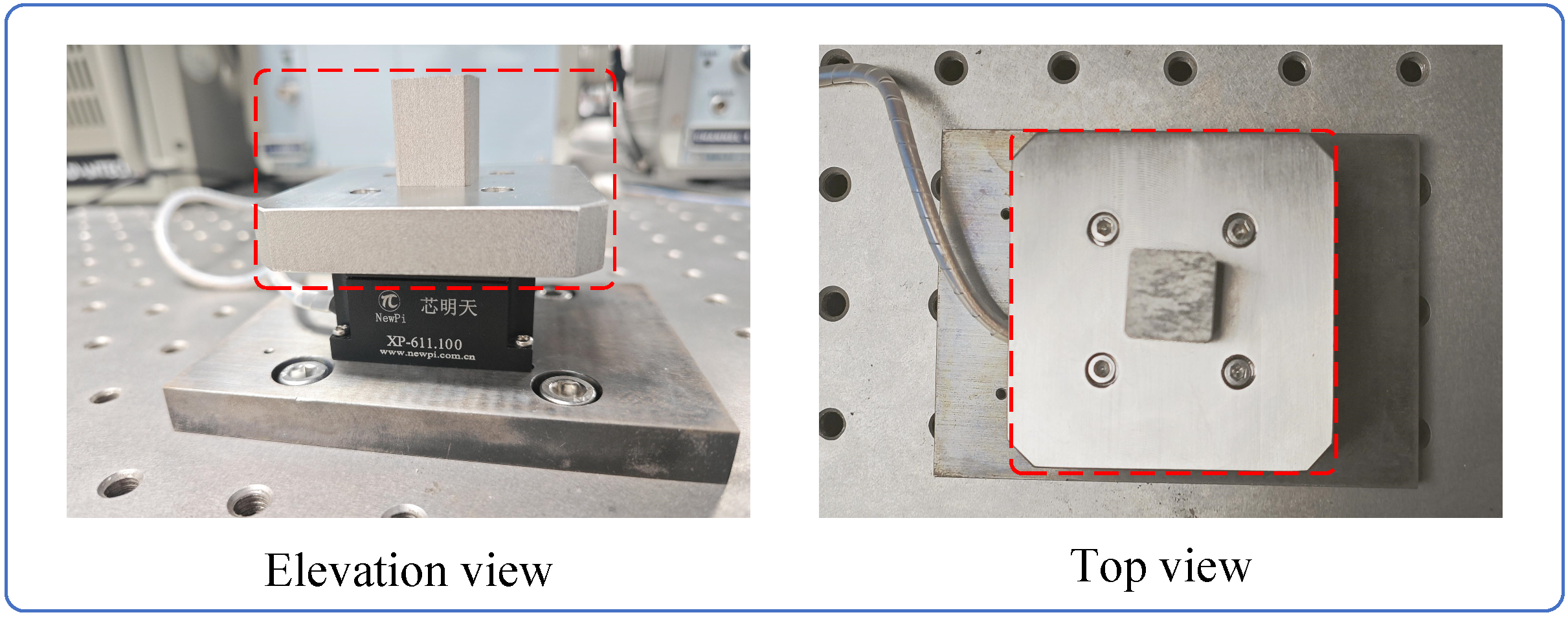
To demonstrate the capability of the proposed control strategy, real-time tracking control experiments were conducted on the experimental platform under two conditions: no-load and with load. The proposed method was compared with the proportional-integral (PI) control based on feedforward hysteresis compensation and the backstepping control (BC) method based on series hysteresis compensation [45]. The load installation setup is shown in Figure 11.
The experimental sampling time was 0.0002 s and the reference displacement signal was set:
r ( t ) = 8 ( 2 sin ( 2 π f t π / 2 ) + 3 ) μ m 8 sin ( 2 π f 1 t ) + sin ( 2 π f 2 t ) cos ( 2 π f 3 t ) + 3 μ m
f = 10 ,   20 ,   40 ,   50   Hz ,   f 1 , 2 , 3 = 5 ,   20 ,   10   Hz   or   10 ,   50 ,   20   Hz .
The controller parameters were set as follows: process noise covariance matrix Qk = 1 × 10⁻⁵ and observation noise covariance matrix Rk = 9 × 10⁻⁸ in the Kalman filter. Q = [100 0; 0 0], R = 2000, A = [0.93 1.767 × 10⁻⁴; −668.761 0.753], B = [0.0695; 663.813], C = [1, 0].

4.2. Experimental Results and Analysis

Figure 12a–f show the experimental results of tracking control without load, including the tracking curve graph and the error curve graph.
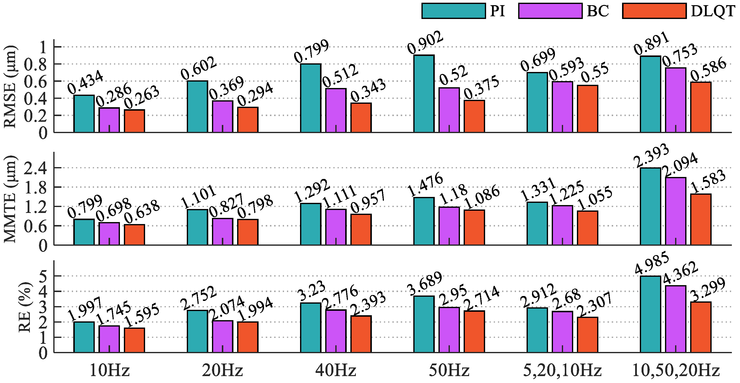
Figure 13 presents the tracking control error metrics under the no-load condition, including the Root Mean Square Error (RMSE), Maximum Tracking Error (MMTE), and Relative Error (RE).
In the no-load real-time tracking experiments, the DLQT control strategy consistently outperforms the PI and BC controllers across various reference displacement signals. Specifically, DLQT reduces RMSE by over 21.3% compared to PI and by more than 7% compared to BC. MMFE is reduced by more than 20% compared to PI (with an average reduction of 25.43%) and by over 3.5% compared to BC (averaging 12.08%). For RE, DLQT achieves an average reduction of 26.17% compared to PI and 11.66% compared to BC. These results demonstrate that the DLQT control strategy proposed in this paper provides superior tracking performance under no-load conditions.
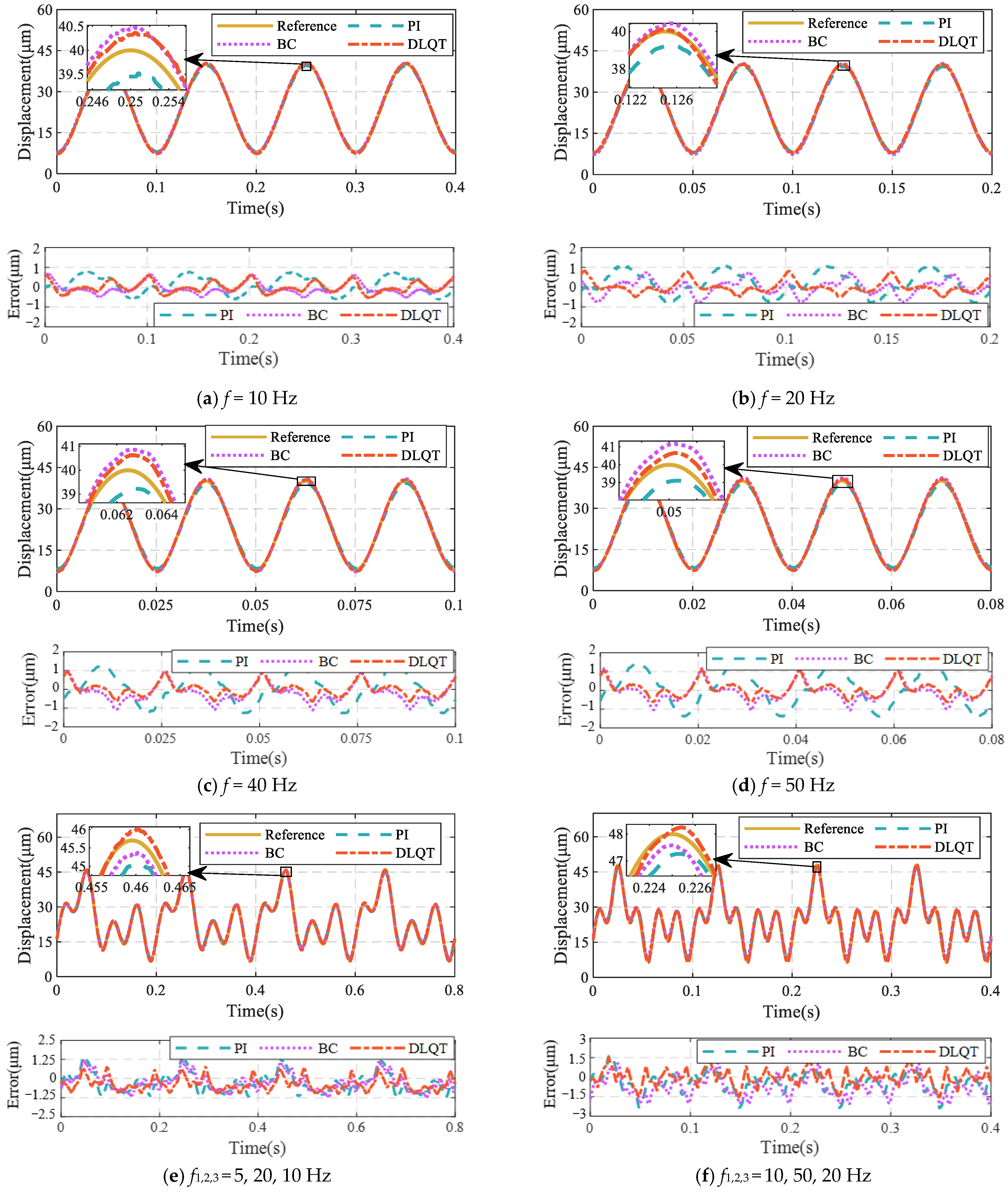
Figure 14a–f presents the experimental results of the tracking control under load conditions, including both the tracking trajectories and the corresponding error curves.
Figure 15 illustrates the error evaluation metrics for the tracking control experiment under load conditions. The results indicate that the DLQT control strategy proposed in this paper consistently outperforms the PI and BC control strategies. After adding the load, the system’s uncertainty and complexity increase, making accurate tracking more difficult, and all three control strategies show increased error indices compared to the no-load case. Nonetheless, the DLQT method still achieves the lowest error metrics. In the tracking experiments with different reference displacement frequencies, the maximum RE values for the PI and BC strategies exceed 6%, while the maximum RE value for the DLQT strategy is only 4.385%. These experimental results and error summary plots demonstrate that the DLQT control strategy can effectively mitigate external disturbances and improve the tracking accuracy and reliability of the piezoelectric actuators.

5. Conclusions

To address the issue of hysteresis nonlinearity affecting the tracking control accuracy of piezoelectric actuators, this paper investigates hysteresis model identification and tracking control strategies. For model identification, a particle swarm optimization (PSO) algorithm with a dual-improvement strategy is proposed. By incorporating a cross-variation mechanism, the algorithm enhances particle diversity during iteration, effectively overcoming the traditional PSO’s tendency toward local optima and premature convergence. Evolutionary factors are introduced to adaptively adjust inertia weights and learning factors, thereby balancing local and global search capabilities and improving both convergence speed and accuracy. Benchmark function optimization tests demonstrate that the improved PSO algorithm outperforms comparative algorithms in terms of convergence speed and accuracy across various benchmark functions. Experimental results of hysteresis model identification show that the proposed algorithm improves identification accuracy by 17.9%, 17.5% and 15.4% compared to comparison algorithm. In terms of tracking control, a hysteresis compensator is first designed based on the identified model to mitigate the system’s hysteresis nonlinearity. A DLQT controller is then developed for the compensated system to enhance tracking performance. Hardware-in-the-loop tracking experiments show that, under no-load conditions, the maximum RMSE and RE of the DLQT controller are 0.586 μm and 3.299%, respectively, for various reference signals. Under load conditions, the maximum RE values are 3.696% for single-frequency and 4.385% for multi-frequency reference signals. These experimental results validate the effectiveness of the proposed control strategy.
The hysteresis compensator developed in this study is based on a rate-independent model, which satisfies the requirements at low and moderate frequencies but shows reduced effectiveness under high-frequency inputs. Future work will focus on developing rate-dependent hysteresis models to further improve compensation performance over a wider frequency range. In addition, adaptive algorithms will be considered to enable real-time tuning of controller parameters, thereby further improving system robustness and control accuracy. Beyond single-degree-of-freedom piezoelectric actuators, the proposed modeling and compensation framework is, in principle, applicable to other hysteretic actuators such as magnetostrictive and shape-memory-alloy devices. Moreover, its extension to multi-degree-of-freedom systems can be achieved through multi-input–multi-output modeling and decoupling control strategies, though this requires further investigation and experimental validation. These directions will contribute to improving both the generalizability and the practical impact of the proposed method.

Author Contributions

Conceptualization, D.L.; methodology, D.L. and X.Z.; software, X.Z. and X.L. (Xuan Li); validation, X.Z. and C.W.; investigation, L.T.; resources, D.L. and S.Y.; data curation, X.L. (Xuejun Li); writing—original draft preparation, X.Z.; writing—review and editing, D.L. and S.Y.; supervision, S.Y.; project administration, D.L. All authors have read and agreed to the published version of the manuscript.

Funding

This research was funded by the Science and Technology Project of the Education Department of Jilin Province, China (Grant No. 2022LY502L17), with a total funding amount of CNY 25,000, supporting seven researchers.

Data Availability Statement

The data presented in this study are available on request from the corresponding author due to privacy and ongoing data management policies governing their public release.

Conflicts of Interest

The authors declare no conflicts of interest.

References

  1. Zhou, X.; Wu, S.; Wang, X.; Wang, Z.; Zhu, Q.; Sun, J.; Huang, P.; Wang, X.; Huang, W.; Lu, Q. Review on piezoelectric actuators: Materials, classifications, applications, and recent trends. Front. Mech. Eng. 2024, 19, 6. [Google Scholar] [CrossRef]
  2. Jin, H.; Gao, X.; Ren, K.; Liu, J.; Qiao, L.; Liu, M.; Chen, W.; He, Y.; Dong, S.; Xu, Z.; et al. Review on piezoelectric actuators based on high-performance piezoelectric materials. IEEE Trans. Ultrason. Ferroelectr. Freq. Control 2022, 69, 3057–3069. [Google Scholar] [CrossRef] [PubMed]
  3. Chang, Q.; Chen, W.; Zhang, S.; Deng, J.; Liu, Y. Review on Multiple-Degree-of-Freedom Cross-Scale Piezoelectric Actuation Technology. Adv. Intell. Syst. 2024, 6, 2300780. [Google Scholar] [CrossRef]
  4. Mei, T.; Huang, K.; Fang, H.; Fan, Q.; Xiao, H.; Xu, Q.; Dai, X.; Yang, Q.; Liu, C. High-precision and large-range deflection of light beams with fast steering mirrors. Opt. Lett. 2024, 49, 5427–5430. [Google Scholar] [CrossRef]
  5. Gao, C.; Zeng, Z.; Peng, S.; Shuai, C. Magnetostrictive alloys: Promising materials for biomedical applications. Bioact. Mater. 2022, 8, 177–195. [Google Scholar]
  6. Li, J.; Zhang, Y.; Yan, M.; Zhong, C.; Zhao, L.; Zhai, D.; Luo, H.; Yuan, X.; Zhang, D. 3D printing of flexible piezoelectric composite with integrated sensing and actuation applications. Adv. Powder Mater. 2024, 3, 100226. [Google Scholar] [CrossRef]
  7. Liang, C.; Sun, F.P.; Rogers, C.A. Dynamic output characteristics of piezoelectric actuators. Smart Struct. Mater. 1993, 1916, 341–352. [Google Scholar]
  8. Chang, F.; Luus, R. A noniterative method for identification using Hammerstein model. IEEE Trans. Autom. Control 2003, 16, 464–468. [Google Scholar] [CrossRef]
  9. Wills, A.; Schön, T.B.; Ljung, L.; Ninness, B. Identification of hammerstein–wiener models. Automatica 2013, 49, 70–81. [Google Scholar] [CrossRef]
  10. Mayergoyz, I.D. Dynamic Preisach models of hysteresis. IEEE Trans. Magn. 2002, 24, 2925–2927. [Google Scholar] [CrossRef]
  11. Oh, J.H.; Bernstein, D.S. Semilinear Duhem model for rate-independent and rate-dependent hysteresis. IEEE Trans. Autom. Control 2005, 50, 631–645. [Google Scholar]
  12. Kanchan, M.; Santhya, M.; Bhat, R.; Naik, N. Application of modeling and control approaches of piezoelectric actuators: A review. Technologies 2023, 11, 155. [Google Scholar] [CrossRef]
  13. Cai, J.; Dong, W.; Nagamune, R. A survey of Bouc-Wen hysteretic models applied to piezo-actuated mechanical systems: Modeling, identification, and control. J. Intell. Mater. Syst. Struct. 2023, 34, 1843–1863. [Google Scholar] [CrossRef]
  14. Zhang, Q. A tutorial on linear least square estimation. arXiv 2022, arXiv:2211.15347. [Google Scholar] [CrossRef]
  15. Chu, S.; Mao, Y.; Dong, Z.; Yang, X. Parameter identification of high-speed USV maneuvering response model based on maximum likelihood algorithm. Acta Armamentarii 2020, 41, 127. [Google Scholar]
  16. Beheshti, Z.; Shamsuddin, S.M.H. A review of population-based meta-heuristic algorithms. Int. J. Adv. Soft Comput. Appl. 2013, 5, 1–35. [Google Scholar]
  17. Alhijawi, B.; Awajan, A. Genetic algorithms: Theory, genetic operators, solutions, and applications. Evol. Intell. 2024, 17, 1245–1256. [Google Scholar] [CrossRef]
  18. Song, Y.; Cai, X.; Zhou, X.; Zhang, B.; Chen, H.; Li, Y.; Deng, W.; Deng, W. Dynamic hybrid mechanism-based differential evolution algorithm and its application. Expert Syst. Appl. 2023, 213, 118834. [Google Scholar] [CrossRef]
  19. Shami, T.M.; El-Saleh, A.A.; Alswaitti, M.; AI-Tashi, Q.; Summakieh, M.A.; Mirjalili, S. Particle swarm optimization: A comprehensive survey. IEEE Access 2022, 10, 10031–10061. [Google Scholar] [CrossRef]
  20. Mirjalili, S.; Mirjalili, S.M.; Lewis, A. Grey wolf optimizer. Adv. Eng. Softw. 2014, 69, 46–61. [Google Scholar] [CrossRef]
  21. Awadallah, M.A.; Makhadmeh, S.N.; Al-Betar, M.A.; Dalbah, L.M.; Al-Redhaei, A.; Kouka, S.; Enshassi, O.S. Multi-objective ant colony optimization. Arch. Comput. Methods Eng. 2025, 32, 995–1037. [Google Scholar] [CrossRef]
  22. Jain, M.; Saihjpal, V.; Singh, N.; Singh, S.B. An overview of variants and advancements of PSO algorithm. Appl. Sci. 2022, 12, 8392. [Google Scholar] [CrossRef]
  23. Shi, Y.; Eberhart, R.C. Empirical study of particle swarm optimization. In Proceedings of the 1999 Congress on Evolutionary Computation-CEC99, Washington, DC, USA, 6–9 July 1999; Volume 3, pp. 1945–1950. [Google Scholar]
  24. Brown, D.F.; Xie, S.Q. A Piecewise Particle Swarm Optimisation Modelling Method for Pneumatic Artificial Muscle Actuators. Actuators 2024, 13, 286. [Google Scholar] [CrossRef]
  25. Zheng, Y.; Wang, Y.; Liu, J. Research on structure optimization and motion characteristics of wearable medical robotics based on Improved Particle Swarm Optimization Algorithm. Future Gener. Comput. Syst. 2022, 129, 187–198. [Google Scholar] [CrossRef]
  26. Fang, S.; Wang, Y.; Wang, W.; Chen, Y.; Chen, Y. Design of permanent magnet synchronous motor servo system based on improved particle swarm optimization. IEEE Trans. Power Electron. 2021, 37, 5833–5846. [Google Scholar] [CrossRef]
  27. Sun, Y.; Wang, X.; Yang, J. Modified particle swarm optimization with attention-based LSTM for wind power prediction. Energies 2022, 15, 4334. [Google Scholar] [CrossRef]
  28. Xiao, J.; Zhang, Z.; Terzi, S.; Anwer, N.; Eynard, B. Dynamic task allocations with Q-learning based particle swarm optimization for human-robot collaboration disassembly of electric vehicle battery recycling. Comput. Ind. Eng. 2025, 204, 111133. [Google Scholar] [CrossRef]
  29. Yu, S.Y.; Feng, Y.Y.; Yang, X.P. Extended state observer–based fractional order sliding-mode control of piezoelectric actuators. Proc. Inst. Mech. Eng. Part I J. Syst. Control Eng. 2021, 235, 39–51. [Google Scholar] [CrossRef]
  30. Liu, H.T.; Zhang, G.L.; Zhou, K.M. Identification of low-damping resonance characteristics and the high-bandwidth control of a piezo-positioning stage. J. Vib. Shock 2024, 43, 287–296. [Google Scholar]
  31. Salah, M.; Saleem, A. Hysteresis compensation-based robust output feedback control for long-stroke piezoelectric actuators at high frequency. Sens. Actuators A Phys. 2021, 319, 112542. [Google Scholar] [CrossRef]
  32. FU, Y.; CHEN, W. Optimal tracking control method for discrete-time linear multivariable systems with decoupling performance. Acta Autom. Sin. 2022, 48, 1931–1939. [Google Scholar]
  33. Argentim, L.M.; Rezende, W.C.; Santos, P.E.; Aparecido Aguiar, R. PID, LQR and LQR-PID on a quadcopter platform. In Proceedings of the 2013 International Conference on Informatics, Electronics and Vision (ICIEV), Dhaka, Bangladesh, 17–18 May 2013; pp. 1–6. [Google Scholar]
  34. Cao, Y.; Ren, W. Optimal linear-consensus algorithms: An LQR perspective. IEEE Trans. Syst. Man Cybern. Part B (Cybern.) 2009, 40, 819–830. [Google Scholar]
  35. Kennedy, J.; Eberhart, R. Particle swarm optimization. In Proceedings of the International Conference on Neural Networks (ICNN’95), Perth, Australia, 27 November–1 December 1995; Volume 4, pp. 1942–1948. [Google Scholar]
  36. Ratnaweera, A. Particle swarm optimization with self-adaptive acceleration coefficients. In Proceedings of the 1st International Conference on Fuzzy Systems and Knowledge Discovery (FSKD 2002), Singapore, 18–22 November 2002; Volume 1, pp. 264–268. [Google Scholar]
  37. Srinivas, M.; Patnaik, L.M. Adaptive probabilities of crossover and mutation in genetic algorithms. IEEE Trans. Syst. Man. Cybern. 1994, 24, 656–667. [Google Scholar] [CrossRef]
  38. Mirjalili, S.; Gandomi, A.H.; Mirjalili, S.Z.; Saremi, S.; Faris, H.; Mirjalili, S.M. Salp Swarm Algorithm: A bio-inspired optimizer for engineering design problems. Adv. Eng. Softw. 2017, 114, 163–191. [Google Scholar] [CrossRef]
  39. Liu, D.; Dong, J.; Guo, S.; Tan, L.; Yu, S. Parameter identification of model for piezoelectric actuators. Micromachines 2023, 14, 1050. [Google Scholar] [CrossRef]
  40. Li, Z.; Xu, R.; Wang, H.N.; Xiong, T. The identification strategy of bouc-wen model based on improved particle swarm optimization algorithm. In Proceedings of the 33rd Chinese Control and Decision Conference (CCDC 2021), Kunming, China, 22–24 May 2021; pp. 6528–6532. [Google Scholar]
  41. Xu, X.; Rong, H.; Trovati, M.; Liptrott, M.; Bessis, N. CS-PSO: Chaotic particle swarm optimization algorithm for solving combinatorial optimization problems. Soft Comput. 2018, 22, 783–795. [Google Scholar] [CrossRef]
  42. Welch, G.; Bishop, G. An Introduction to the Kalman Filter; The University of North Carolina at Chapel Hill: Chapel Hill, NC, USA, 1995. [Google Scholar]
  43. Liu, Z.; Xu, X.; Guo, J.; He, Y.; Zhuang, Y.; Yu, S. Damping force tracking control of magnetorheological damper based on Koopman operators. Control Theory Appl. 2024, 1–11. Available online: https://link.cnki.net/urlid/44.1240.TP.20241010.1652.014 (accessed on 1 October 2025).
  44. Liu, B.; Tang, W. Modern Control Theory; China Machine Press: Beijing, China, 2006. [Google Scholar]
  45. Qiao, J.H. Backstepping Control Method and Implementation, 1st ed.; China Machine Press: Beijing, China, 2012; pp. 21–24. [Google Scholar]
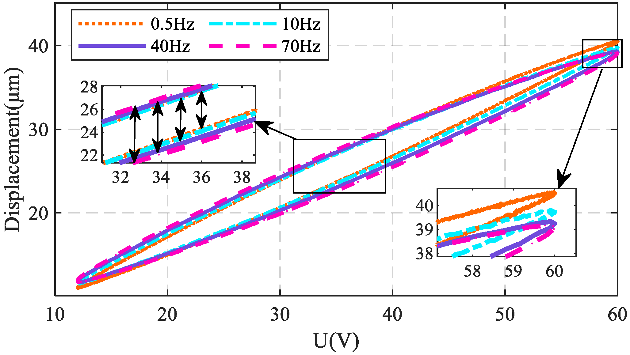
Figure 1. Frequency-dependent hysteresis curves of input voltage and output displacement of the piezoelectric actuator.
Processes 13 03212 g001
Figure 3. (a) Three-dimensional images for different benchmark functions (The coloring is used only to visually distinguish function magnitudes: red = high, blue = low); (b) Optimal value iteration curve; (c) Optimal value logarithmic iteration curve.
Processes 13 03212 g003
Figure 4. Experimental platform for piezoelectric actuators.
Processes 13 03212 g004
Figure 5. Real-time working principle diagram of the piezoelectric actuator platform.
Processes 13 03212 g005
Figure 6. Iteration curves of fitness function values for asymmetric bouc-wen model parameter identification using different pso algorithms.
Processes 13 03212 g006
Figure 7. Hysteresis loops for 0.5 Hz systems corresponding to different algorithms.
Processes 13 03212 g007
Figure 8. Comparison of hysteresis loop curves obtained from experimental platform and hammerstein model under different excitation frequencies: (a) 5 Hz, (b) 20 Hz, (c) 40 Hz, and (d) 50 Hz.
Processes 13 03212 g008
Figure 9. Piezoelectric actuators tracking control structure.
Processes 13 03212 g009
Figure 10. Hysteresis compensation structure of the piezoelectric actuator based on a series inverse hysteresis model.
Processes 13 03212 g010
Figure 11. Load installation view.
Processes 13 03212 g011
Figure 12. Experimental results of no-load tracking control.
Processes 13 03212 g012
Figure 13. Tracking control error under no load.
Processes 13 03212 g013
Figure 14. Experimental results of tracking with load.
Processes 13 03212 g014
Figure 15. Tracking control error under load.
Processes 13 03212 g015
Table 1. Parameter settings of the standard PSO and the proposed PSO in benchmark function tests.
MethodParameter Settings
S&RT = 300, S = 40, D = n = 5, ω max = 0.9 ,   ω min = 0.4 ,   c max = 2.5 ,   c min = 0.4
LiuT = 300, S = 40, D = n = 5, ω max = 0.9 ,   ω min = 0.4 ,   c 1 s = 4 ,   c 1 f = 1 ,   c 2 s = 1 ,   c 2 f = 4 ,   P c = P m = 0.2
LiT = 300, S = 40, D = n = 5, ω max = 0.9 ,   ω min = 0.4 ,   c 1 nt = 2 ,   c 1 fin = 4 ,   c 2 int = 2 ,   c 2 fin = 4.5
OurT = 300, S = 40, D = n = 5, ω max = 0.9 ,   ω min = 0.4 , c1 and c2 are shown in Equation (8).
Table 2. Benchmark function optimisation test errors of four PSO algorithms.
Function S&RLiuLiOur
F1Best1.4337 × 10−61.3816 × 10−74.2809 × 10−101.1202 × 10−62
Average3.4861 × 10−79.3276 × 10−73.9715 × 10−96.7365 × 10−59
Std4.5334 × 10−72.0364 × 10−78.7832 × 10−104.9113 × 10−60
F2Best8.9185 × 10−42.0018 × 10−71.7446 × 10−71.9621 × 10⁻¹⁴
Average9.5461 × 10−43.9654 × 10−68.4981 × 10−63.7619 × 10⁻¹³
Std2.3782 × 10−58.9723 × 10−79.2365 × 10−72.9946 × 10⁻¹⁴
F3Best7.4398 × 10−62.1724 × 10−73.8459 × 10−101.0498 × 10⁻²¹
Average9.3972 × 10−51.9527 × 10−66.6498 × 10−119.8951 × 10⁻¹⁹
Std2.7861 × 10−55.9434 × 10−76.5228 × 10−116.0572 × 10⁻²⁰
F4Best2.8238 × 10−51.1436 × 10−74.5237 × 10−81.8025 × 10⁻¹¹
Average8.5928 × 10−53.8249 × 10−62.9746 × 10−68.3268 × 10⁻¹⁰
Std2.1733 × 10−51.2829 × 10−66.9835 × 10−71.1327 × 10⁻¹⁰
F5Best9.2254 × 10−52.0069 × 10−61.7834 × 10−67.5495 × 10⁻¹⁵
Average6.3481 × 10−41.3256 × 10−56.7739 × 10−64.2289 × 10⁻¹⁴
Std1.7883 × 10−43.1394 × 10−61.2198 × 10−62.4026 × 10⁻¹⁵
F6Best7.4068 × 10−24.4367 × 10−26.6499 × 10−22.4644 × 10⁻²
Average9.2329 × 10−26.6854 × 10−27.8826 × 10−23.9771 × 10⁻²
Std8.5073 × 10−36.4164 × 10−32.0182 × 10−31.0566 × 10⁻³
Table 3. Identification errors of Bouc-Wen model identified by the S&R, Liu, Li, and Our PSO algorithms compared with the reference model.
MethodMMFE (μm)RMSE (μm)RE (%)
S&R0.81840.30752.01
Liu0.80130.29642.00
Li0.79780.28351.95
Ours0.66690.25591.65
Table 4. Fitting errors between the Hammerstein model and the experimental platform under different input signal frequencies.
FrequencyMMFE (μm)RMSE (μm)RE (%)
5 Hz0.70350.29521.7587
20 Hz0.90690.40532.2649
40 Hz0.94280.47382.3918
50 Hz1.18340.60412.9916
Disclaimer/Publisher’s Note: The statements, opinions and data contained in all publications are solely those of the individual author(s) and contributor(s) and not of MDPI and/or the editor(s). MDPI and/or the editor(s) disclaim responsibility for any injury to people or property resulting from any ideas, methods, instructions or products referred to in the content.