An End-to-End Framework for Spatiotemporal Data Recovery and Unsupervised Cluster Partitioning in Distributed PV Systems

Abstract

The growing penetration of distributed photovoltaic (PV) systems presents significant operational challenges for power grids, driven by the scarcity of historical data and the high spatiotemporal variability of PV generation. To address these challenges, we propose Generative Reconstruction and Adaptive Identification via Latents (GRAIL), a unified, end-to-end framework that integrates generative modeling with adaptive clustering to discover latent structures and representative scenarios in PV datasets. GRAIL operates through a closed-loop mechanism where clustering feedback guides a cluster-aware data generation process, and the resulting generative augmentation strengthens partitioning in the latent space. Evaluated on a real-world, multi-site PV dataset with a high missing data rate of $45.4\%$, GRAIL consistently outperforms both classical clustering algorithms and deep embedding-based methods. Specifically, GRAIL achieves a Silhouette Score of 0.969, a Calinski–Harabasz index exceeding $4.132\times {10}^6$, and a Davies–Bouldin index of $0.042$, demonstrating superior intra-cluster compactness and inter-cluster separation. The framework also yields a normalized entropy of $0.994$, which indicates highly balanced partitioning. These results underscore that coupling data generation with clustering is a powerful strategy for expressive and robust structure learning in data-sparse environments. Notably, GRAIL achieves significant performance gains over the strongest deep learning baseline that lacks a generative component, securing the highest composite score among all evaluated methods. The framework is also computationally efficient. Its alternating optimization converges rapidly, and clustering and reconstruction metrics stabilize within approximately six iterations. Beyond quantitative performance, GRAIL produces physically interpretable clusters that correspond to distinct weather-driven regimes and capture cross-site dependencies. These clusters serve as compact and robust state descriptors, valuable for downstream applications such as PV forecasting, dispatch optimization, and intelligent energy management in modern power systems.

1. Introduction

Global photovoltaic (PV) deployment has scaled at an unprecedented pace, with over 600 GW added in 2024 and cumulative installations surpassing 2.2 TW; China alone contributed 357.3 GW in 2024 and now hosts about half of global distributed PV capacity [1,2]. At high penetration, the integration of distributed PV introduces significant operational challenges, as its strong spatial heterogeneity, meteorology-driven intermittency, and potential for bidirectional or reverse flows complicate grid planning, dispatch, and protection [3,4,5,6]. These operational hurdles are compounded by fundamental data limitations. Incomplete measurements, sensor noise, and high dimensionality reduce system observability and hinder centralized optimisation [7,8]. Meanwhile, a broadening set of downstream systems depends on compact and reliable PV encodings. For instance, graph-based forecasting leverages spatiotemporal couplings yet often assumes complete observations [9]. Similarly, electric vehicle (EV) planning and demand response require tractable inputs [10,11,12,13,14], power–transport co-optimisation needs concise supply-side descriptions [15,16], and large-scale system models and regional resource studies further underscore the need for low-dimensional, robust, and physically meaningful representations that remain stable under noise and sparsity [17,18,19,20].

To address these intertwined operational and data constraints, clustering has become a critical technique in the distributed PV domain [21,22,23]. By grouping geographically dispersed stations that exhibit similar generation patterns, clustering facilitates a reduction in system dimensionality while preserving behavioral diversity. This in turn supports scalable planning, enhances dispatch coordination, and enables more structured control strategies. A wide range of clustering methods has been applied to PV systems. Centroid-based algorithms like K-means [24] and K-medoids [25] are widely utilized for their efficiency in tasks such as weather-based forecasting and regional output estimation [26,27]. Density-based approaches such as Density-Based Spatial Clustering of Applications with Noise (DBSCAN) [28] and Clustering by Fast Search and Find of Density Peaks (CFSFDP) [29] excel at identifying irregularly shaped clusters for applications like site selection and fault diagnosis [29,30]. Furthermore, fuzzy clustering techniques can model the transitional behavior of PV systems under uncertainty [31,32]. More advanced deep and hybrid models capture complex nonlinear patterns for dynamic scheduling, real-time state evaluation, and weather classification [33,34,35], while hierarchical methods improve granularity for tasks like PV-battery sizing [36].

Despite this progress, existing analytical pipelines for distributed PV face several fundamental limitations. Many clustering and forecasting approaches presuppose complete datasets and rely on ad-hoc preprocessing for missing values, a practice that can introduce bias and obscure true operational patterns. Decoupled workflows that first impute data and then perform clustering are prone to propagating reconstruction errors into the final partitioning. Furthermore, classical algorithms such as k-means or k-medoids are sensitive to scaling and outliers. At the same time, density-based methods require delicate hyperparameter tuning and may classify a large fraction of data as noise, leading to unstable results [24,25,28]. These challenges are compounded by issues of computational cost and interpretability. Heavy sequence encoders can incur high latency and memory footprints, hindering their deployment on edge devices or in real-time environments [37]. Crucially, the latent features produced by many deep models are often not aligned with physical, weather-driven regimes or cross-site couplings. This means they provide limited guidance for dispatch and planning, despite the well-documented spatiotemporal variability of PV resources [18,38,39].

These persistent gaps motivate the development of an integrated, end-to-end framework that couples data generation with clustering. To this end, we propose Generative Reconstruction and Adaptive Identification via Latents (GRAIL), a unified framework that jointly integrates data generation, feature representation, and clustering within a closed-loop optimization paradigm. GRAIL is specifically designed to overcome three fundamental limitations of existing PV clustering approaches, including the reliance on complete datasets, the separation of modeling stages, and a lack of adaptivity to high-dimensional, heterogeneous spatiotemporal patterns. In its iterative pipeline, GRAIL processes incomplete PV sequences using a cluster-aware Recurrent Neural Network (RNN)-based generator that imputes missing observations by leveraging regime-specific dynamics. A jointly trained autoencoder then extracts low-dimensional embeddings that preserve both reconstructive fidelity and clustering structure, enhanced by a cluster regularization term. These learned representations are passed to a Hierarchical Density-Based Spatial Clustering of Applications with Noise (HDBSCAN) algorithm for adaptive partitioning. The partitioning is then refined using a k-Nearest Neighbors (k-NN) algorithm to enhance cluster completeness. Crucially, the resulting cluster assignments are fed back to the generator as conditioning signals in the subsequent iteration, establishing a mutual refinement loop that progressively improves both the latent representations and the generative outputs. This tightly coupled interplay enables GRAIL to robustly extract semantically coherent clusters from noisy, sparse, and nonlinear PV datasets.

The main contributions of this paper are summarized as follows.

• Closed-loop integration of generation and clustering. We introduce a unified learning framework that tightly couples cluster-aware data generation with latent-space clustering through an iterative feedback mechanism. This design promotes mutual reinforcement between generation and partitioning, which mitigates the error propagation common in decoupled pipelines.
• Mask-aware generation for incomplete PV data. We develop a cluster-conditioned Long Short-Term Memory (LSTM) generator with a mask-guided loss function that explicitly prioritizes the recovery of missing entries. This formulation improves imputation fidelity and supports robust temporal modeling in the presence of extensive data sparsity.
• Adaptive density-based clustering with refinement. We employ an HDBSCAN algorithm to detect latent cluster structures without predefining the number of clusters. A k-NN voting scheme is further introduced to reassign samples initially labeled as noise, thereby enhancing spatial consistency and robustness to outliers.

The remainder of this paper is structured as follows. Section 2 introduces the proposed GRAIL framework, detailing its three interdependent modules and the iterative optimization mechanism. Section 3 presents the data preprocessing, experimental setup, evaluation metrics, and a comprehensive comparison and in-depth analysis of GRAIL’s performance. Finally, Section 4 provides a concluding discussion.

2. Materials and Methods

This section details the architecture of the proposed GRAIL framework. We first provide an overview of the overall structure, followed by an elaboration on the three constituent modules: cluster-aware data generation, latent feature representation, and adaptive clustering with refinement. The section concludes with a description of the training procedure.

2.1. Overall Framework

The proposed GRAIL framework unifies cluster-aware data generation, latent feature representation, and adaptive clustering with refinement within a closed-loop, iterative architecture. An overview of the architecture is illustrated in Figure 1. The methodology is organized into three core components, where Module I handles data generation, Module II manages latent feature representation, and Module III performs adaptive clustering. The corresponding learning routine is detailed in Algorithm 1. The process commences with input sequences accompanied by binary masks that indicate missing temporal observations. These masked sequences are first processed by a cluster-aware generator that synthesizes complete trajectories conditioned on evolving latent cluster embeddings. The reconstructed sequences then serve as input to the latent feature representation module, where an encoder extracts low-dimensional embeddings jointly optimized for reconstruction fidelity and cluster discriminability. Subsequently these embeddings are utilized by the adaptive clustering module, which employs density-based partitioning and refinement to identify underlying group structures. The three modules are integrated and co-optimized through a feedback mechanism, depicted by the dashed arrow in Figure 1 and detailed in Algorithm 1 (lines 7–26). In this process predicted cluster assignments are embedded and routed back to the generator to condition the next round of reconstructions. This iterative interaction allows the discovered cluster structure to guide data generation, while the augmented observations in turn help refine the latent representations. Through this synergistic loop, the modules mutually reinforce one another, progressively improving both reconstruction and clustering performance. This study targets non-adversarial data imperfections that commonly occur in distributed PV operations, including stochastic missingness and measurement noise. The framework explicitly models missingness via mask-aware generation and density-adaptive clustering. Our dataset indeed exhibits a high missing-data rate of 45.4%. We do not assume worst-case adversarial perturbations or targeted data poisoning in the current scope. By design, GRAIL is unsupervised and is purposely formulated without direct irradiance inputs. Its mask-aware generator and density-adaptive clustering operate on meteorological and temporal covariates to recover weather-regime structures when irradiance series are absent or unreliable. This approach ensures the method remains deployable in common field conditions while preserving physical interpretability. The resulting clusters align with weather-driven regimes such as clear-sky versus overcast profiles with distinct meteorological signatures, providing a physically grounded basis for generalization. The alternating optimization stabilizes within approximately six outer iterations, indicating computational efficiency.

2.2. Module I: Cluster-Aware Data Generation

Module I of the GRAIL framework functions as a sequence generator designed to reconstruct complete photovoltaic time-series windows from incomplete observations. This generator is both cluster-aware and mask-conditioned. Cluster-aware signifies that the reconstruction is conditioned on the current cluster identity of a given sequence. In this process, a discrete cluster label is mapped to a learnable embedding vector, which is then concatenated with the input at every time step along with a binary observation mask. By incorporating both the cluster context and the explicit missingness pattern, the generator produces sequences that are not only complete but also semantically enriched and structurally coherent within each cluster. These resulting gap-free windows improve data quality and serve as the input for the subsequent representation learning module, thereby closing the loop between generation and clustering.

As visualized in the blue block of Figure 1 and detailed in lines 7–13 of Algorithm 1, this module reconstructs each partially observed window by conditioning on the current cluster identity. Let ${\mathbf{x}}_i\in {\mathbb{R}}^{T\times d}$ be the i-th input window with a corresponding binary mask ${\mathbf{m}}_i\in {\{0,1\}}^{T\times d}$. In this mask, $m_{itj}=1$ indicates an observed entry for window i at time step t and feature index j, while $m_{itj}=0$ indicates a missing entry. The framework segments the input into fixed-length windows as specified in line 4 of Algorithm 1. Each window i is assigned a discrete cluster label $c_i\in \{1,\dots ,K\}\cup \{-1\}$ that is inferred by the clustering module described in Section 2.4, where a label of -1 denotes noise. Conditioning is implemented using a learnable lookup table $\mathbf{E}\in {\mathbb{R}}^{K\times d}$. This embedding matrix maps the discrete label $c_i$ to a continuous vector ${\mathbf{e}}_{c_i}$. This vector is then concatenated with the input at every time step in ${\mathbf{x}}_i$, as shown in line 10 of Algorithm 1, to form an enriched sequence input for the generator:

$${\widehat{\mathbf{x}}}_i=G_{\psi }({\mathbf{x}}_i,{\mathbf{m}}_i,{\mathbf{e}}_{c_i}).$$

(1)

This conditioning allows the LSTM-based generator to adapt its behavior to cluster-level priors such as geographic regime and weather pattern, yielding reconstructions that are coherent within each cluster.

Algorithm 1: Generative Reconstruction and Adaptive Identification via Latents (GRAIL)

To avoid biasing the model toward already observed entries, supervision is restricted to only the missing components. With indices i for windows, t for time steps, and $j\in \{1,\dots ,d\}$ for features, the loss for Module I is defined as

$${\mathcal{L}}_{\mathrm{generation}}={\displaystyle \frac{1}{{\sum }_{i,t,j}(1-m_{itj})}}\sum _{i,t,j}(1-m_{itj}){(x_{itj}-{\widehat{x}}_{itj})}^2,$$

(2)

As illustrated in Figure 1, this mask-aware formulation ensures that gradients propagate only through unobserved components, which prevents trivial reconstructions and encourages semantically meaningful imputations. Because the binary mask ${\mathbf{m}}_i$ is provided as an input to the generator $G_{\psi }$ and is also used to restrict supervision, the model inherently adapts to arbitrary, site-specific patterns of missing data.

In practice, the generator $G_{\psi }$ is implemented as a sequence model capable of capturing local temporal dependencies. Our implementation employs LSTM [40], although alternative architectures such as a Gated Recurrent Unit (GRU) [41] or Transformer [42] can be adopted without affecting the framework’s generality. We select LSTM for its practical advantages over these alternatives. It is computationally efficient with linear runtime and memory requirements suitable for deployment, in contrast to the quadratic complexity of Transformers [42,43]. LSTM is also a proven and stable method for time-series imputation when data gaps are contiguous, a characteristic common in real-world PV operational datasets [44], and it generally offers better control over long-range information than GRU [45,46,47]. Crucially, the integration of cluster embeddings and a selective gradient flow allows the generator to learn latent dynamics that are robust to both noise and sparsity. As described in line 13 of Algorithm 1, the model parameters $\mathit{\psi }$ are updated via back-propagation through the masked reconstruction loss.

2.3. Module II: Latent Feature Representation

Module II of the GRAIL framework, illustrated by the yellow block in Figure 1 and formalized in lines 16–18 of Algorithm 1, encodes the reconstructed input sequences into compact and semantically structured representations. Unlike generic dimensionality reduction techniques, this module is explicitly designed to support the dual objectives of reconstruction fidelity and clustering alignment. It thereby serves as a critical bridge between low-level temporal dynamics and high-level structural semantics.

Given a synthesized sequence ${\mathbf{x}}_i\in {\mathbb{R}}^{T\times d}$ from Module I, an encoder $f_{\theta }(·)$ maps the sequence to a latent code ${\mathbf{z}}_i\in {\mathbb{R}}^{d_z}$, which is subsequently processed by a decoder $g_{\varphi }(·)$ to yield the reconstructed sequence ${\widehat{\mathbf{x}}}_i$:

$${\mathbf{z}}_i=f_{\theta }\left({\mathbf{x}}_i\right),{\widehat{\mathbf{x}}}_i=g_{\varphi }\left({\mathbf{z}}_i\right).$$

(3)

This encoder–decoder pair is trained jointly using a composite objective function:

$${\mathcal{L}}_{\mathrm{total}}={\mathcal{L}}_{\mathrm{AE}}+{\lambda }_c·{\mathcal{L}}_{\mathrm{cluster}},$$

(4)

the first term, $\mathcal{L}\mathrm{AE}$, ensures that the latent representation retains adequate information from the input by promoting accurate sequence reconstruction. It is formulated as a mean squared error (MSE) loss:

$${\mathcal{L}}_{\mathrm{AE}}={\displaystyle \frac{1}{n}}\sum _{i=1}^n{\parallel {\mathbf{x}}_i-{\widehat{\mathbf{x}}}_i\parallel }_2^2,$$

(5)

which encourages the preservation of temporal signal features during the encoding process, as depicted by the “reconstruction-guided encoding” arrow in Figure 1.

The second term, ${\mathcal{L}}_{\mathrm{cluster}}$, promotes semantic coherence and structural separability by penalizing the intra-cluster variance in the latent space:

$${\mathcal{L}}_{\mathrm{cluster}}={\displaystyle \frac{1}{K}}\sum _{k=1}^K{\displaystyle \frac{1}{|C_k|}}\sum _{{\mathbf{z}}_i\in C_k}{\parallel {\mathbf{z}}_i-{\mathit{\mu }}_k\parallel }_2^2,$$

(6)

where K is the number of non-noise clusters identified by HDBSCAN, $C_k=\{i:c_i=k\}$ is the index set of samples in cluster k and ${\mathit{\mu }}_k$ denotes the centroid of cluster k in the latent space.

This composite objective guides the latent space to become both reconstructive and cluster-discriminative. The balance between its two terms is controlled by the hyperparameter ${\lambda }_c$, as illustrated beneath Module II in Figure 1 and in line 18 of Algorithm 1.

A key aspect of the training process is that this module is optimized progressively across the outer iterations of the framework, and its parameters are not reset. This cumulative optimization allows the latent manifold to evolve in tandem with the generator and clustering modules. Such an approach stabilizes the representation learning process, prevents model collapse, and progressively enhances the semantic granularity of the embeddings.

2.4. Module III: Adaptive Clustering with Refinement

As illustrated in the red block of Figure 1 and detailed in lines 19–26 of Algorithm 1, Module III performs density-based clustering on the latent representations ${\left\{{\mathbf{z}}_i\right\}}_{i=1}^n$ to discover the underlying group structure within the distributed PV data. Unlike conventional clustering routines, this module serves a dual purpose. It not only determines the final pseudo-labels for downstream use but also closes the framework’s iterative loop by feeding these cluster labels back into the generator.

The core of this module is the HDBSCAN algorithm, which is applied to the encoded features ${\left\{{\mathbf{z}}_i\right\}}_{i=1}^n\subset {\mathbb{R}}^{d_z}$ from Module II.

$$c_i=\mathcal{H}\left({\mathbf{z}}_i\right),$$

(7)

where $c_i\in \{1,2,\dots ,K\}\cup \{-1\}$ denotes the cluster label, and $-1$ marks a sample as noise. To automatically determine the optimal clustering scale, the algorithm performs a grid search over a set of candidate min_cluster_size values $\{s_1,\dots ,s_m\}$, as demonstrated in line 21 of Algorithm 1. For each setting, HDBSCAN first constructs a mutual-reachability graph:

$$d_{\mathrm{mreach}}(x_i,x_j)=max\left\{{\mathrm{core}}_k\left(x_i\right),{\mathrm{core}}_k\left(x_j\right),\parallel x_i-x_j\parallel \right\},$$

(8)

where ${\mathrm{core}}_k\left(x\right)$ is the distance to the k-NN, an adaptive metric that enables the detection of clusters with heterogeneous densities.

The resulting hierarchical cluster tree is pruned using a stability-based selection criterion, where the stability of a cluster C is measured as

$$\mathrm{Stability}\left(C\right)={\int }_{{\lambda }_{\mathrm{birth}}}^{{\lambda }_{\mathrm{death}}}\left|C\left(\lambda \right)\right|d\lambda ,$$

(9)

where $\lambda =1/\delta$ is the inverse density, $\delta$ is the distance, and $\left|C\right(\lambda \left)\right|$ is the cluster size at that level. The configuration yielding the maximal global stability is selected to produce the final cluster assignments ${\left\{c_i\right\}}_{i=1}^n$, as shown in line 23 of Algorithm 1.

To enhance the completeness of this partitioning, GRAIL applies k-NN refinement for noise points, as illustrated in lines 24–26 of Algorithm 1. Specifically, for any noisy point, the label $c_i=-1$ is reassigned based on the majority label of theirs k closest non-noise neighbors:

$$c_i=\mathrm{mode}\left\{c_j\mid j\in {\mathcal{N}}_k\left(i\right),c_j\ne -1\right\}.$$

(10)

This correction promotes spatial smoothness and enhances the completeness of cluster assignments.

The refined cluster assignments are then used to inform the next generative iteration. Each cluster label is mapped to a continuous representation ${\mathbf{e}}_{c_i}\in {\mathbb{R}}^d$ via a trainable embedding matrix $\mathbf{E}\in {\mathbb{R}}^{K\times d}$:

$${\mathbf{e}}_{c_i}=\mathbf{E}[c_i,:],$$

(11)

which is routed back to Module I to condition subsequent data generation, ensuring mutual alignment among the generation, representation, and clustering modules.

Overall, this feedback loop highlights the dual function of Module III. It not only produces cluster labels $c_i$ that supervise representation learning via the cluster compactness loss ${\mathcal{L}}_{\mathrm{cluster}}$, but also guides the generator through embedding feedback. By combining adaptive density modeling, noise-aware refinement, and loop-level feedback, module III enables GRAIL to autonomously extract compact, robust, and semantically coherent clusters from incomplete and noisy PV datasets.

2.5. Iterative Training Procedure

Rather than optimizing each module in isolation, GRAIL adopts an alternating update scheme across its generation, representation, and clustering modules. This tightly coupled design forms a closed-loop feedback architecture that progressively enhances data fidelity, latent space compactness, and structural coherence.

As outlined in Algorithm 1, training begins with a pre-processing step (lines 1–4), which includes zero-imputation and fixed-window segmentation of the PV datasets. Model parameters for the generator $\mathit{\psi }$, encoder $\mathit{\theta }$, and decoder $\mathit{\varphi }$ are randomly initialized (line 5). Initial cluster assignments $c_i$ are set to $-1$ to indicate a state of uncertainty.

The core training procedure unfolds over I outer iterations (line 6), with each iteration comprising three interdependent steps. First, the generator reconstructs missing values based on the current cluster embeddings. These generated sequences are then fed into the encoder to produce latent representations. Finally, the latent features are used to infer cluster structures through adaptive density-based clustering. This iterative process is closed by the feedback mechanism, as illustrated in Figure 1. The updated cluster assignments $\left\{c_i\right\}$ are embedded into vectors $\left\{{\mathbf{e}}_{c_i}\right\}$ using a learnable matrix, and these embeddings are routed back to the generator to guide the subsequent round of data synthesis.

This closed-loop structure enables mutual reinforcement across modules. As the clustering becomes more stable, the generation improves because the cluster embeddings more accurately reflect the underlying operational regimes. Better generation yields higher-quality inputs for representation learning. In turn, improved representations support more coherent and compact clustering. Through this feedback cycle, GRAIL progressively aligns data quality, feature consistency, and structural interpretability. The process also does not require a predefined number of clusters or other manually specified structural priors.

In practice, the model typically converges within a few outer iterations, outputting the reconstructed sequences $\widehat{\mathbf{X}}$, informative latent codes $\mathbf{Z}$ and robust cluster assignments $\mathbf{C}$ as returned in line 27 of Algorithm 1.

Unlike conventional pipelines that treat imputation, representation, and clustering as separate steps, GRAIL integrates these components into a unified training loop. Each module builds upon the outputs of the others while preserving its learned parameters across iterations. This continuity avoids the instability associated with random reinitialization and helps maintain long-range dependencies and semantic coherence. The result is a stable and effective training process that can uncover interpretable structures in noisy and incomplete PV datasets.

3. Results

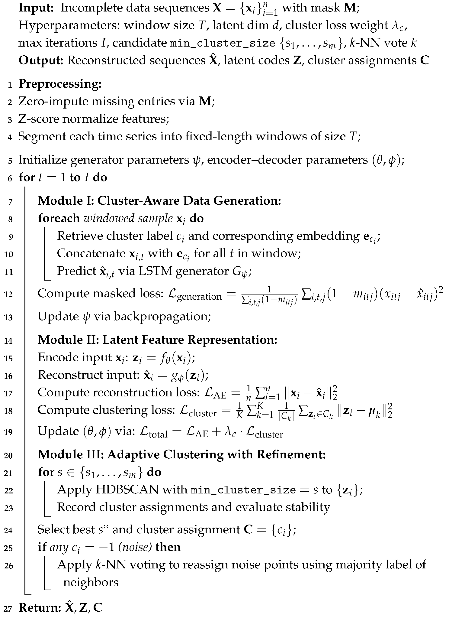
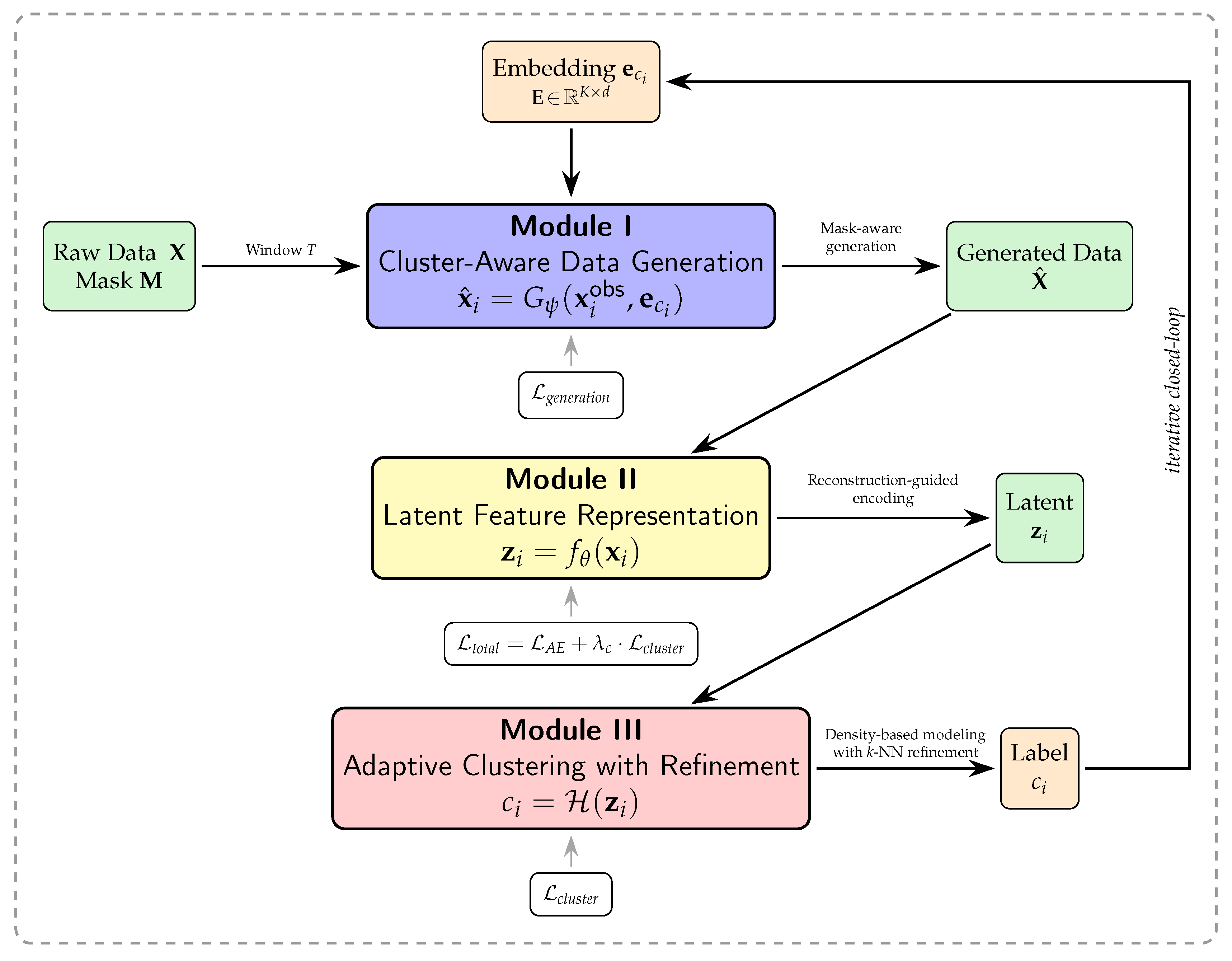
This section presents a comprehensive evaluation of the proposed GRAIL framework using a real-world distributed photovoltaic dataset. We begin by describing the dataset and the preprocessing pipeline. We then introduce the evaluation metrics, present a comparative analysis of GRAIL against several baseline models, and conclude with an in-depth analysis of the framework’s performance.

3.1. Data

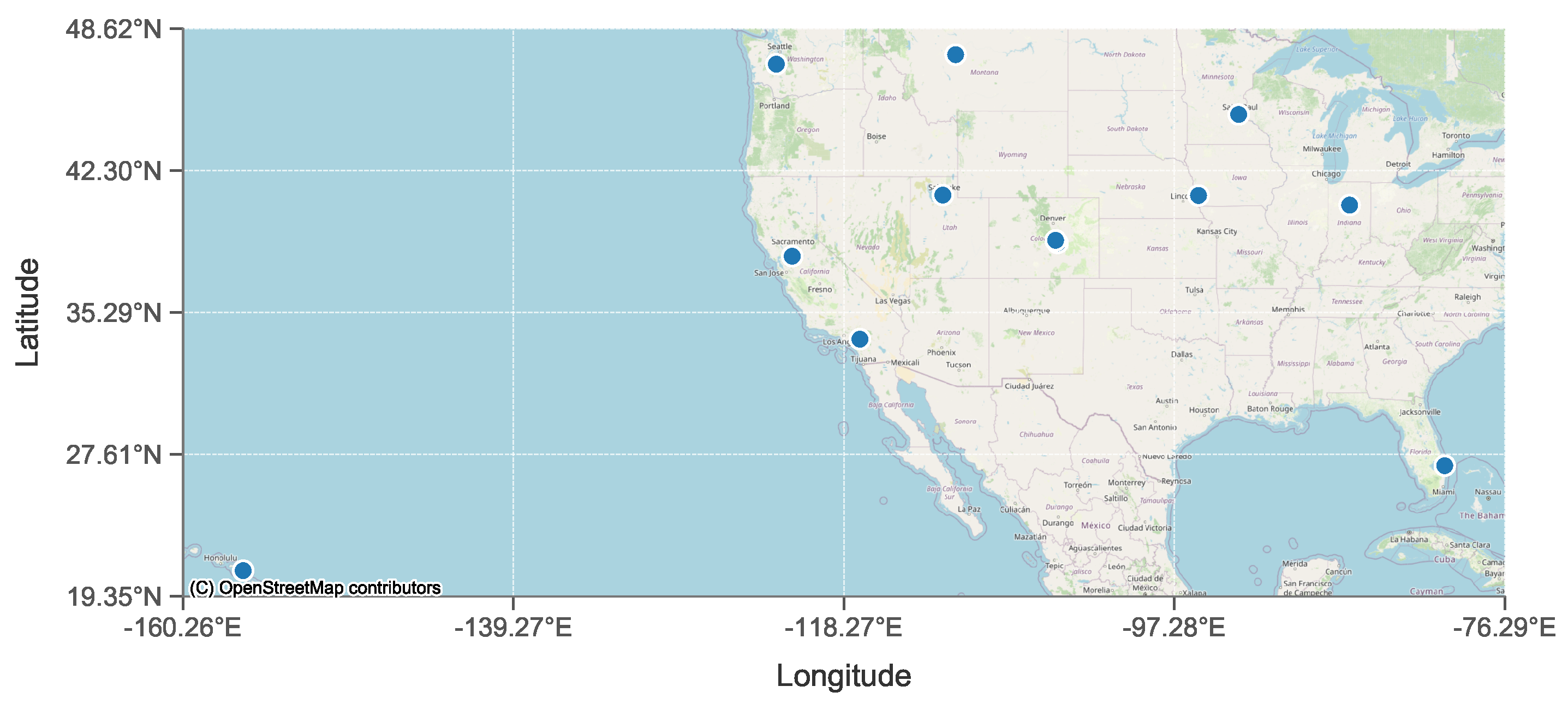
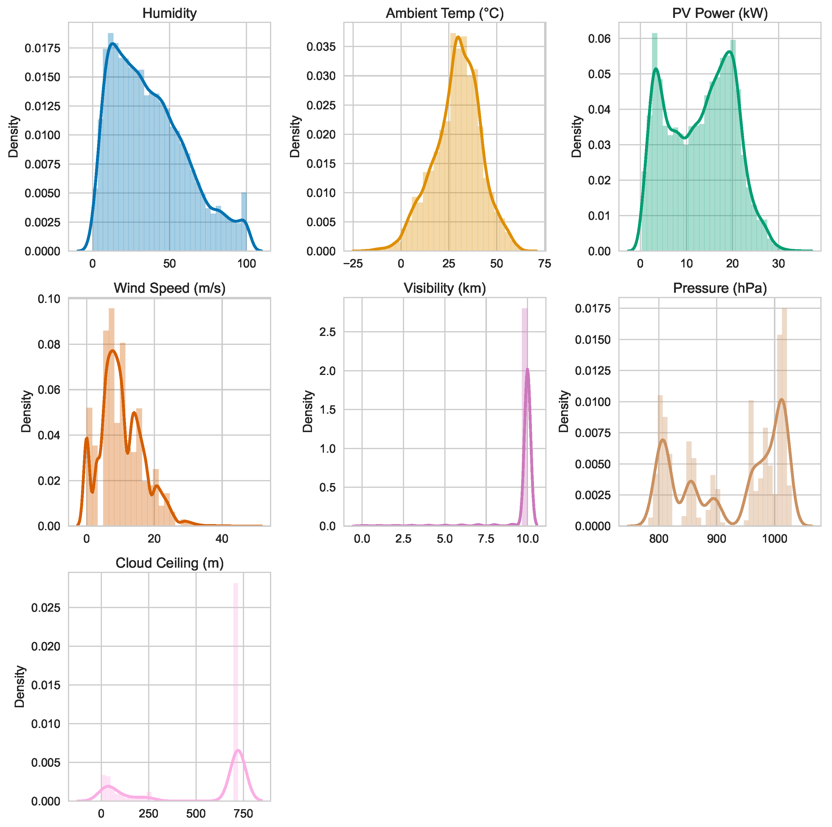
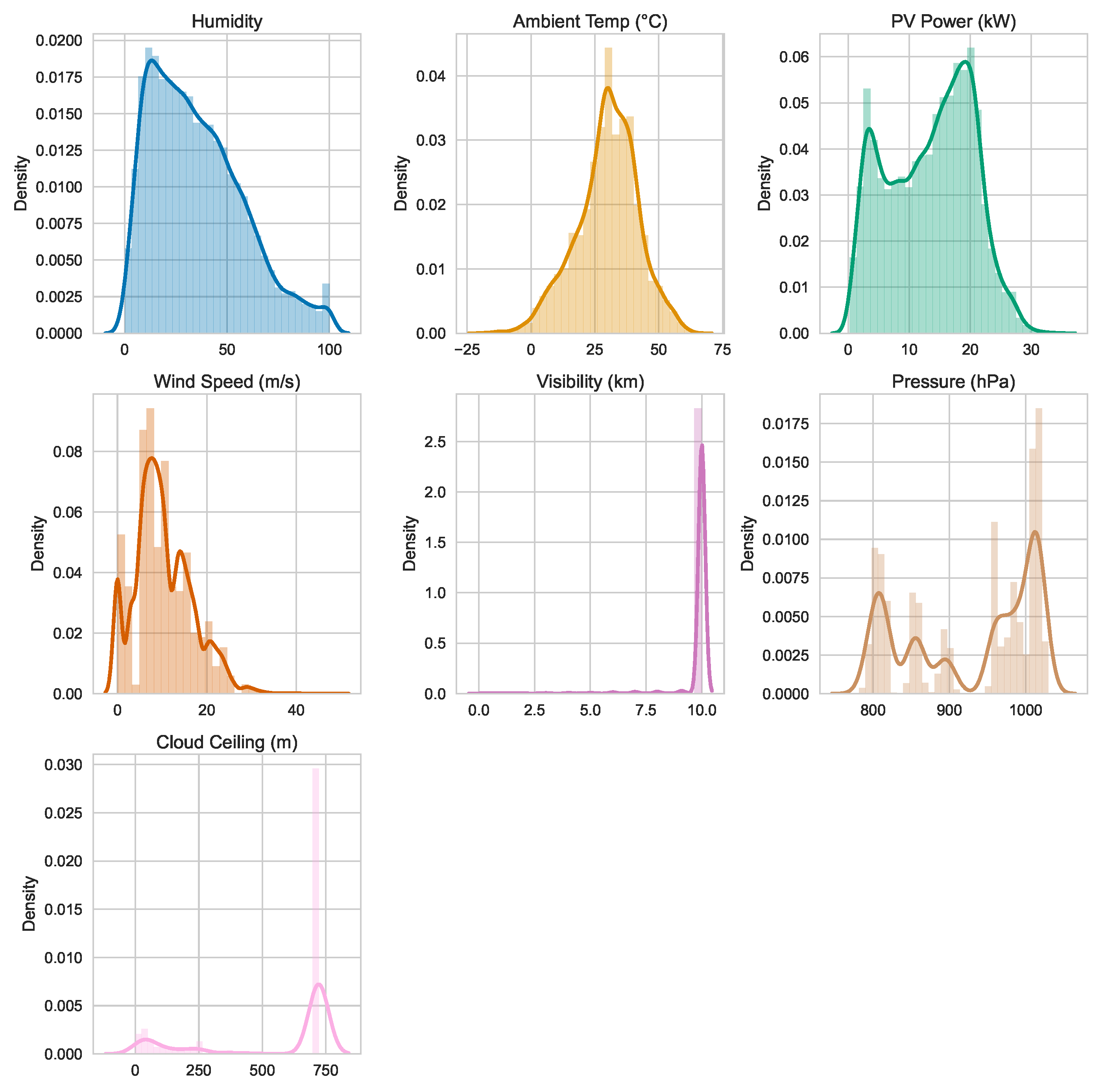
The dataset employed in this study consists of multi-site spatiotemporal records collected from horizontal photovoltaic panels deployed across 12 distinct locations in the Northern Hemisphere, covering a continuous 14-month observation period. As visualized in Figure 2, the sites span a broad geographic range from approximately 160° W to 76° W longitude and 19° N to 48° N latitude, encompassing diverse coastal, island, and inland settings. Each observation contains 17 raw features, including meteorological covariates like humidity, ambient temperature, wind speed, visibility, surface pressure, and cloud ceiling, which exhibit wide variability, as shown in Figure 3, Figure 4 and Figure 5. This environmental and geographic diversity, compounded by a substantial missing data rate of 45.4%, presents a realistic and challenging scenario reflective of heterogeneous operating conditions in distributed PV fleets. These characteristics motivate the development of methods that are robust to both data sparsity and cross-site variability. The specific sites analyzed are Camp Murray, Grissom, Hill Weber, JDMT, Kahului, MNANG, Malmstrom, March AFB, Offutt, Peterson, Travis, and USAFA.

Notably, the dataset does not contain direct measurements of solar irradiance. This omission is by design and reflects common operational conditions where irradiance series are frequently unavailable or unreliable due to factors such as sensor outages, soiling, calibration drift, and biases in satellite or reanalysis products [38,39,48]. Since solar irradiance is a dominant driver of PV generation, its absence poses a realistic and nontrivial modeling challenge. Our study explicitly targets this irradiance-scarce regime. The proposed framework is designed to infer irradiance-dependent dynamics solely from other observable environmental covariates and latent cross-site structural information. This capability is critical for developing robust models that can be deployed in practical settings where high-quality irradiance data cannot be guaranteed.

To balance temporal resolution with computational efficiency, the original PV data sampled at 15-min intervals, shown in Figure 3, are aggregated into hourly windows using mean pooling as illustrated in Figure 4. This results in a total of 18,312 aggregated samples. A visual comparison of the marginal distributions before and after this process confirms that the statistical properties of the resampled data remain highly consistent with the original series across all numerical predictors. This consistency indicates that key temporal and meteorological patterns are well preserved after aggregation, supporting the suitability of hourly-resolution data for the subsequent modeling.

The dataset also exhibits considerable heterogeneity in temporal coverage and data completeness across the different sites, as shown in

Table 1. Effective periods across twelve photovoltaic sites.

Location	Start Time	End Time	Record Count
Camp Murray	13 December 2017 11:45	2 October 2018 15:00	1113
Grissom	7 November 2017 11:00	4 October 2018 13:30	1487
Hill Weber	19 June 2017 15:00	4 October 2018 15:00	2384
JDMT	23 May 2017 11:00	24 May 2018 10:00	1779
Kahului	3 November 2017 10:00	13 June 2018 14:00	941
MNANG	9 November 2017 10:00	2 October 2018 14:00	780
Malmstrom	31 October 2017 10:00	30 September 2018 12:15	1517
March AFB	6 July 2017 13:00	2 October 2018 15:00	2204
Offutt	1 April 2018 10:00	27 September 2018 15:00	881
Peterson	29 May 2017 10:00	27 September 2018 15:00	2640
Travis	9 June 2017 11:00	3 October 2018 14:00	2746
USAFA	25 May 2017 10:00	1 October 2018 14:00	2573

. The start and end timestamps of data collection vary significantly among locations, reflecting differences in sensor deployment timelines and operational stability. To mitigate this temporal misalignment and ensure consistent coverage, a common subwindow from 1 December 2017 10:00:00 to 1 June 2018 15:00:00 is selected, yielding a dataset of 7192 hourly observations. The statistical distribution of this final dataset, shown in Figure 5, remains aligned with both the original 15-min and the aggregated hourly data, confirming the validity of the selected subwindow for a cross-site comparative analysis.

Despite temporal alignment, the refined dataset exhibits substantial sparsity. Within the selected time frame, an expected count of 13,176 hourly records is present for a complete dataset. However, only 7192 valid observations exist, which indicates a high missingness rate of 45.4%. This degree of incompleteness underscores the critical need for modeling techniques capable of operating effectively under conditions of severe data sparsity. The GRAIL framework, enabling effective modeling under severe data absence by capturing shared temporal dynamics and latent variability structures across space and time, is capable of solving the problem.

To enhance the temporal representativeness and modeling efficacy of the aggregated hourly dataset, we perform feature engineering and standardization. First, a suite of calendar-based features is derived to enrich the temporal context of each observation, including IsWeekend, Month, Day, Hour, DayOfWeek, DayOfYear, and WeekOfYear. Predictors designed by feature engineering capture distinct aspect of temporal periodicity relevant to photovoltaic output dynamics, respectively.

To encode the cyclical nature inherent in attributes mentioned above, sine and cosine transformations are applied as follows:

$$x_{sin}=sin\left({\displaystyle \frac{2\pi x}{P}}\right),x_{cos}=cos\left({\displaystyle \frac{2\pi x}{P}}\right),$$

(12)

where x denotes a time-based feature and P is the corresponding period. Specifically, we use P = 6 for Hour feature (reflecting the key 10:00 to 15:00 operational window), P = 7 for DayOfWeek, and P = 365 for DayOfYear. This transformation maps discrete time indices onto the unit circle, preserving continuity and facilitating smooth transitions for temporal modeling. Such encoding scheme is advantageous for RNN architecture that benefits from continuous and differentiable inputs. Conversely, the Year attribute is excluded from the final feature set. Its variance over the 2017–2018 sampling window is negligible, rendering it uninformative for learning meaningful temporal patterns.

All continuous numerical variables are standardized using z-score normalization:

$${x_i}^{\prime }={\displaystyle \frac{x_i-\mu }{\sigma }},$$

(13)

where $\mu$ and $\sigma$ represent the empirical mean and standard deviation the feature, respectively.

This normalization procedure places all inputs on a comparable scale. As a result, it improves numerical stability, reduces the model’s sensitivity to initial parameter values, and can accelerate convergence during training.

After data preprocessing, the resulting dataset comprises 7192 hourly samples, each with 25 features. These features can be categorized into three groups:

• Spatiogeographic Descriptors including Location, Latitude, Longitude, and Altitude.
• Meteorological and PV Measurements including Season, Humidity, AmbientTemperature, PowerOutput, WindSpeed, Visibility, Pressure, and CloudCeiling.
• Temporal Encodings including IsWeekend, Month_sin, Month_cos, Day_sin, Day_cos, Hour_sin, Hour_cos, DayOfWeek_sin, DayOfWeek_cos, DayOfYear_sin, DayOfYear_cos, WeekOfYear_sin, and WeekOfYear_cos.

The enriched feature space provides the foundation for the GRAIL framework to learn latent irradiance-sensitive dynamics from auxiliary environmental and calendar signals, even in the absence of direct solar irradiance measurements.

3.2. Experiment

To systematically evaluate the performance of various clustering algorithms on spatiotemporal photovoltaic data, a comprehensive benchmark across eight representative methods is conducted. These comparators are selected to instantiate four orthogonal axes of the design space. The first axis is the algorithmic family, spanning partition-based, density-based, and hierarchical density approaches. The second axis is the data representation, distinguishing between classical methods operating on raw features and deep methods using autoencoder latent embeddings. A third axis is the training paradigm, which contrasts two-stage deep embedding with joint optimisation. The final axis is the use of generative augmentation. This taxonomy covers the classic-to-deep spectrum relevant to unsupervised PV clustering under missing data. The first group consists of classical algorithms K-means, DBSCAN, and HDBSCAN. The second category comprises deep clustering approaches DE-KMeans, DE-DBSCAN, DE-HDBSCAN, DEC-HDBSCAN, and our proposed GRAIL framework.

Table 2. Training paradigms and embedding strategies of the evaluated clustering methods.

Model	Category	Training Paradigm	Embedding Strategy
K-means	Classic	Partition-based	Raw
DBSCAN	Classic	Density-based	Raw
HDBSCAN	Classic	Hierarchical density	Raw
DE-KMeans	Deep	Two-stage (AE pretrain → K-means)	AE latent (frozen after pretraining)
DE-DBSCAN	Deep	Two-stage (AE pretrain → DBSCAN)	AE latent (frozen after pretraining)
DE-HDBSCAN	Deep	Two-stage (AE pretrain → HDBSCAN)	AE latent (frozen after pretraining)
DEC-HDBSCAN	Deep	Joint optimisation (AE + clustering loss)	AE latent (jointly refined by clustering loss)
GRAIL (ours)	Deep	Joint optimisation (Generation + AE + HDBSCAN)	AE latent (Generation-augmented, jointly refined by clustering loss)

Abbreviations: AE = autoencoder; DE = Deep Embedded; DEC = Deep Embedded Clustering.

summarises the mapping of these models to the design axes. Furthermore, to isolate the effect of the generator, we also evaluate a no-generation configuration where the generator is disabled and incomplete data is handled via listwise deletion. The results of this analysis are presented in Section 3.4.2.

The hyperparameters in Algorithm 1 are configured with specific default values and initialization strategies. The input window length T is set to 32. For the LSTM generator, evaluation of recurrent depths ℓ from $\{1,2,3\}$ and hidden sizes h from $\{64,128,256\}$ shows no significant accuracy differences. To balance runtime and memory, we adopt a shallow configuration with $\ell =2$, a hidden size of $h=128$, and a dropout rate of $0.2$. This choice maintains framework generality since the model is agnostic to the specific recurrent design [45] and aligns with prior photovoltaic forecasting practices that often use shallow LSTM to mitigate overfitting and meet deployment constraints [38]. Each cluster label is mapped to a learnable embedding of dimension $d_e=8$ through a table $\mathbf{E}\in {\mathbb{R}}^{K\times d_e}$. For a sample window with label $c_i$, the conditioning vector $e_{c_i}$ is concatenated to every time step and then fed to the generator. The embedding table $\mathbf{E}$ is initialized using Xavier-uniform initialization with zero biases. We apply a mild ${\ell }_2$ penalty on $\mathbf{E}$ and a small dropout with $p=0.1$ on $e_{c_i}$ to reduce overfitting in sparsely observed clusters. A default value of $d_e=8$ is chosen because a sensitivity check over $\{4,8,16\}$ shows negligible differences and offers a favorable latency-memory trade-off. The autoencoder’s latent dimension $d_z$ is set to 10, while additional ablation studies evaluate values of 8 and 16. The training process runs for $I=20$ outer iterations. The clustering-consistency weight ${\lambda }_c$ is initialized at 1.0 and annealed using a piecewise schedule. It is set to 1.0 for iterations 1 to 5, 0.5 for iterations 6 to 10, 0.2 for iterations 11 to 15, and 0.1 for iterations 16 to 20. For HDBSCAN, we scan the min_cluster_size over twenty logarithmically spaced candidates ranging from 0.1% to 50% of the total number of sites N. We select the solution located in a stability plateau that maximizes cluster persistence. The min_samples hyperparameter is set to 10 by default and is tuned over values of 3, 5, 10, and 20. After clustering, points labeled as noise are reassigned using a k-NN majority vote with $k=5$, while values of 3, 7, and 11 are also evaluated. Models are trained using the Adam optimizer with a learning rate of ${10}^{-3}$ and a weight decay of ${10}^{-5}$. A StepLR scheduler is applied with a step_size of 5 and a $\gamma$ of 0.5. The batch size is 16 for the RNN generator and 128 for the autoencoder. Both components are trained for 10 epochs within each outer iteration. All networks are randomly initialized and initial cluster labels are set to $-1$. Random seeds are fixed to ensure reproducibility. We conduct further sensitivity studies by varying T across $\{24,32,48\}$, I across $\{8,12,20\}$, and ${\lambda }_c$ across $\{1.0,0.5,0.2,0.1\}$ while repeating the HDBSCAN searches described previously.

For all models employing an HDBSCAN clustering head, the min_cluster_size is determined by sweeping over 20 logarithmically spaced candidates between $0.1\%$ and $50\%$ of the dataset size N. The min_samples parameter is tuned from the set $\{3,5,10,20\}$. Any points initially labeled as noise are subsequently reassigned using a k-NN majority vote, with k selected from $\{3,5,7,11\}$. All neural network-based models are trained using the Adam optimizer with a learning rate of $1\times {10}^{-3}$ and a weight decay of $1\times {10}^{-5}$, paired with a StepLR scheduler configured with a step size of 5 and a decay factor $\gamma$ of 0.5. The cluster-embedding dimension is set to $d_e=8$ and the autoencoder latent size to $d_z=10$. Unless stated otherwise, experiments are run for $I=20$ outer iterations using an input window length of $T=32$. Within each outer iteration, the LSTM generator is trained for 10 epochs with a batch size of 16, while the autoencoder is trained for 10 epochs with a batch size of 128. The clustering-consistency weight ${\lambda }_c$ is annealed from $1.0$ to $0.1$ across the iterations. For the classical baselines, the K-means algorithm is implemented with K-means++ initialization, and the number of clusters K is selected via the elbow method. For DBSCAN, the min_samples parameter is fixed at 5, and the neighborhood radius $ϵ$ is chosen from a grid guided by an analysis of k-distance plots.

K-means is a canonical partitioning algorithm that minimizes intra-cluster variance by iteratively assigning samples to the nearest centroid. Since the number of clusters must be predefined, we determine this hyperparameter by applying the elbow method to a candidate range of cluster counts. To enhance stability and mitigate sensitivity to initial conditions, we employ the K-means++ initialization heuristic, which improves convergence and reduces the likelihood of settling in suboptimal local minima.

DBSCAN represents a classical density-based algorithm, excels at discovering clusters of arbitrary shape without requiring a predefined cluster count. It identifies clusters by connecting high-density regions, governed by a neighborhood radius $ϵ$ and a minimum point count  min_samples. In our implementation, min_samples is set to 5, and the radius is selected via a grid search informed by k-distance plots, which help estimate the intrinsic neighborhood scale of the data. To mitigate fragmentation from points classified as noise, a post-processing step reassigns these outliers based on a majority vote among their nearest non-noise neighbors, thereby improving cluster completeness and spatial coherence.

HDBSCAN extends DBSCAN by introducing a hierarchical, density-based framework that adapts to clusters of varying densities without requiring a strict distance threshold. This makes it particularly well-suited for complex, heterogeneous data distributions. Its primary hyperparameters, including the minimum cluster size, are optimized via a grid search over a range proportional to the dataset size. A refinement step is also applied to relabel ambiguous points initially marked as noise, enhancing the structural integrity of the final partitioning.

DE-KMeans follows a two-stage paradigm that decouples representation learning from clustering. First, an autoencoder is trained to map the raw input data into a compact latent space, capturing a denoised and task-relevant structure. The K-means algorithm is then applied to partition the resulting latent embeddings. This design leverages the power of deep feature extraction while retaining the simplicity of centroid-based clustering. The number of clusters is determined using the elbow method, and the latent space remains fixed during clustering to ensure stable and reproducible results.

DE-DBSCAN substitutes the centroid-based K-means in the DE-KMeans pipeline with a density-based alternative. By applying DBSCAN to the learned latent space, this method can identify non-convex and irregularly shaped clusters. The autoencoder is trained to compress the input sequences into a semantically structured embedding space, where DBSCAN operates using a fixed minimum point count and a neighborhood radius selected via k-distance analysis.

DE-HDBSCAN advances the deep density-based approach by coupling HDBSCAN with the latent embeddings from an autoencoder. This pairing enables the discovery of multi-scale density structures within a compact and robust feature space. The minimum cluster size is optimized through a grid search over logarithmically spaced values. To suppress over-fragmentation, a minimum number of core neighbors is specified, and ambiguous points are relabeled using nearest-neighbor voting.

DEC-HDBSCAN represents a more integrated paradigm where feature learning and clustering are jointly optimized. The model first initializes cluster assignments using HDBSCAN on the latent representations. It then iteratively refines both the cluster assignments and the autoencoder’s parameters using a clustering-aware loss, which encourages the encoder to learn more discriminative features. The primary hyperparameter is the minimum cluster size, which is selected by scanning over a predefined range during initialization.

GRAIL, in contrast to approaches that separate representation learning and clustering, performs a unified, end-to-end optimization. Each experiment consists of 20 outer iterations, with each iteration comprising three sequential stages. In the first stage, An LSTM-based recurrent neural network reconstructs missing values within fixed-length input windows of 32 time steps. To make the generation cluster-aware, each sequence is augmented at every time step with a trainable 8-dimensional embedding corresponding to its current cluster identity. Specifically, a discrete label $c_i$ is mapped via an embedding table $\mathbf{E}\in {\mathbb{R}}^{K\times d_e}$ to a vector $e_{c_i}\in {\mathbb{R}}^{d_e}$, which is then fed to the generator. A binary mask distinguishes observed from missing entries, and the network is trained for 10 epochs using a masked mean squared error objective to optimize only the imputed values. In the second stage, the imputed sequences are processed by an autoencoder, which projects the inputs into a 10-dimensional latent space. The autoencoder is trained for 10 epochs per iteration using a composite loss that balances reconstruction fidelity with a cluster-consistency regularizer. This regularizer encourages samples from the same cluster to form compact regions in the latent space. Crucially, network parameters are preserved across iterations, allowing for progressive refinement of the latent structure. In the third stage, HDBSCAN is applied to the latent embeddings to partition the data. A grid search over 20 candidate values for the minimum cluster size, logarithmically spaced between 0.1% and 50% of the dataset size, is performed to accommodate clusters of varying density. Finally, to improve assignment coverage, a 5-nearest-neighbor majority vote is used to reassign any points initially labeled as noise.

3.3. Evaluation

To systematically evaluate clustering performance, we adopt a multi-indicator framework integrating four complementary metrics: Silhouette Score, Calinski–Harabasz index, Davies–Bouldin index, and normalized clustering entropy. Each metric assesses a different aspect of partitioning quality, from geometric separation to distributional balance.

The Silhouette Score (S) quantifies the quality of a clustering by measuring how similar a sample is to its own cluster compared to other clusters. It is calculated for each sample and then averaged over all samples as follows:

$$S={\displaystyle \frac{1}{n^{\prime }}}\sum _{i=1}^{n^{\prime }}{\displaystyle \frac{b_i-a_i}{max(a_i,b_i)}},$$

(14)

where $a_i$ is the average intra-cluster distance for sample i, and $b_i$ is its average distance to the nearest neighboring cluster. A score near $+1$ indicates dense, well-separated clusters.

The Calinski–Harabasz index (C), also known as the variance ratio criterion, measures the ratio of between-cluster dispersion to within-cluster dispersion. It is defined as:

$$C={\displaystyle \frac{\mathrm{Tr}\left(B_k\right)}{\mathrm{Tr}\left(W_k\right)}}·{\displaystyle \frac{n-k}{k-1}},$$

(15)

where $\mathrm{Tr}\left(B_k\right)$ and $\mathrm{Tr}\left(W_k\right)$ are the traces of the between-cluster and within-cluster scatter matrices, respectively, k is the number of clusters, and n is the total number of samples. Higher Calinski–Harabasz index values indicate better-defined clusters.

The Davies–Bouldin index (D) evaluates cluster separation by computing the average similarity between each cluster and its most similar counterpart. It is defined as:

$$D={\displaystyle \frac{1}{k}}\sum _{i=1}^k\underset{j\ne i}{max}\left({\displaystyle \frac{s_i+s_j}{d_{ij}}}\right),$$

(16)

where $s_i$ is the average distance of points in cluster i to their centroid, and $d_{ij}$ denotes the Euclidean distance between the centroids of clusters i and j. Lower values of D indicate better inter-cluster dissimilarity and more compact clusters.

Normalized entropy (H) measures the uniformity of the sample distribution across clusters. It is computed as:

$$H=-\sum _{i=1}^k{p}_{i}log\left(p_i\right)/log\left(k\right),\mathrm{where}{p}_i={\displaystyle \frac{n_i}{n}},$$

(17)

where $n_i$ is the number of samples in cluster i, and n is the total number of samples. A value near 1 implies that clusters are of a similar size, indicating a balanced partitioning.

To aggregate these metrics into a unified ranking criterion, we employ min–max normalization across each score and define a weighted composite score (M):

$$M=w_s·\tilde{S}+w_c·\tilde{C}+w_d·(1-\tilde{D})+w_h·\tilde{H},$$

(18)

where $\tilde{S}$, $\tilde{C}$, $\tilde{D}$, $\tilde{H}$ are the normalized versions of the corresponding metrics, and $(w_s,w_c,w_d,w_h)=(0.4,0.3,0.2,0.1)$ reflect the relative importance attributed to silhouette coherence and inter-cluster separation over statistical balance and compactness.

3.4. Model Comparison

3.4.1. Models with Generative Augmentation

The quantitative comparison presented in

Table 3. The performance of clustering models with data Generation.

Model/Metric	S	C	D	H	Composite Score	Ranking
K-means	0.122	1.812 × 103	2.270	0.984	0.163	7
DBSCAN	0.078	1.564 × 103	3.484	0.977	0.059	8
HDBSCAN	0.216	3.956 × 103	1.781	0.999	0.261	4
DE-KMeans	0.185	3.390 × 103	1.714	0.960	0.179	6
DE-DBSCAN	0.322	6.484 × 103	1.337	0.949	0.242	5
DE-HDBSCAN	0.421	6.442 × 103	1.336	0.945	0.279	3
DEC-HDBSCAN	0.956	6.711 × 105	0.066	0.971	0.690	2
GRAIL (Our)	0.969	4.132 × 106	0.042	0.994	0.991	1

Bold indicates the best result; underlined indicates the second-best.

reveals significant variation in clustering performance across models. Classical methods such as K-means and DBSCAN demonstrate limited clustering capability, with Silhouette Scores of 0.122 and 0.078, and relatively low Calinski–Harabasz indices of $1.81\times {10}^3$ and $1.56\times {10}^3$, respectively, indicating weak inter-cluster separation. The Davies–Bouldin indices of 2.270 and 3.484 suggest high intra-cluster dispersion. Although their normalized entropy values of 0.984 and 0.977 imply balanced cluster sizes, this uniformity may obscure poor semantic structure or reflect fragmentation into similarly sized but incoherent regions, particularly in the case of DBSCAN. HDBSCAN demonstrates improved geometric separability, with a Silhouette Score of 0.216 and a moderately higher Calinski–Harabasz index of $3.96\times {10}^3$. However, its entropy further increases to 0.999, suggesting highly uniform but potentially over-fragmented partitions with limited semantic cohesion.

To better leverage structure-preserving properties of latent representations, deep embedded clustering variants are further evaluated. DE-KMeans and DE-DBSCAN both improve intra-cluster compactness of 1.714 and 1.337, and Silhouette Scores of 0.185 and 0.322. DE-DBSCAN achieves a more favorable balance between density sensitivity and feature expressiveness, yielding a normalized entropy of 0.949 and a Calinski–Harabasz index of $6.48\times {10}^3$. DE-HDBSCAN further improves separation and compactness, achieving a Silhouette Score of 0.421 and Davies-–Bouldin index of 1.336, though its entropy slightly decreases to 0.945, indicating mild cluster size imbalance in exchange for enhanced geometric regularity.

Further, DEC-HDBSCAN achieves stronger joint optimization of clustering and representation. With a Silhouette Score of 0.956, Calinski–Harabasz index of $6.71\times {10}^5$, and compactness score of 0.066, it demonstrates well-separated and coherent partitions. Its entropy of 0.971 remains moderate, reflecting that clusters are slightly unbalanced in size but structurally well-formed.

Moreover, the proposed GRAIL framework attains the best overall performance, with a Silhouette Score of 0.969, Calinski–Harabasz index of $4.13\times {10}^6$, and a Davies–Bouldin index of 0.042. It consistently outperforms all baselines in both separation and compactness. Importantly, its normalized entropy of 0.994 confirms that clusters are not only geometrically well-formed but also highly uniform in size distribution. This balance highlights the advantage of closed-loop integration of cluster-guided generation, reconstruction-aware representation, and density-based refinement.

To provide a unified evaluation metric, we construct Composite Score M by applying min–max normalization and linearly aggregating the Silhouette Score, Calinski–Harabasz index, inverse Davies–Bouldin index, and normalized entropy, with weights specified in Section 3.3. As reported in Table 3, GRAIL achieves the highest Composite Score of 0.991, significantly outperforming the second-best method DEC-HDBSCAN, which attains Composite Score of 0.69. In contrast, classical algorithms such as K-means with a score of 0.163 and DBSCAN with a score of 0.059 exhibit lower composite scores, which underscore the limited expressive capacity and structural rigidity of traditional clustering techniques when applied to complex high-dimensional spatiotemporal PV data.

3.4.2. Models Without Generative Augmentation

To further examine the impact of data generation for clustering, we also evaluate a non-generative configuration. In this setting, the generator is disabled. Instead of imputing missing values, we perform complete-case filtering by discarding any sample window containing one or more missing entries. Given the dataset’s 45.4% missingness rate, this procedure substantially reduces the number of usable samples and may introduce a bias toward sites with more complete observations. The remaining complete windows are fed directly to the autoencoder for deep methods, while baseline models operate on the raw features. All other preprocessing steps and hyperparameters are held constant. This listwise deletion strategy provides a conservative performance baseline. As shown in

Table 4. The performance of clustering models without data Generation.

Model/Metric	S	C	D	H	Composite Score	Ranking
K-means	0.122	1.009 × 103	2.275	0.961	0.158	6
DBSCAN	0.047	3.222 × 102	4.645	0.999	0.100	7
HDBSCAN	0.221	2.201 × 103	1.770	0.990	0.291	4
DE-KMeans	0.172	1.559 × 103	1.587	0.970	0.232	5
DE-DBSCAN	0.223	2.314 × 103	1.683	0.999	0.313	3
DE-HDBSCAN	0.289	3.388 × 103	1.382	0.992	0.345	2
DEC-HDBSCAN	0.909	2.546 × 105	0.132	0.953	0.900	1

Bold indicates the best result; underlined indicates the second-best.

, the performance of classical methods is notably constrained under this setting. K-means achieves a modest Silhouette Score of 0.122 and a Calinski-Harabasz index of $1.009\times {10}^3$, coupled with a relatively high Davies-Bouldin index of 2.275. DBSCAN, by contrast, attains the lowest Composite Score of 0.1, a result attributable to an undesirable Silhouette Score of 0.047 and an extremely high Davies-Bouldin index of 4.645, which indicate excessive noise labeling and unstable cluster boundaries. HDBSCAN also performs modestly. Its high normalized entropy of 0.990 suggests that it produces highly uniform but potentially over-segmented cluster sizes.

The deep embedded methods show marked improvement over classical techniques, though they also reveal certain trade-offs. While DE-KMeans and DE-DBSCAN surpass their classical counterparts, their performance is mixed. Specifically, DE-DBSCAN achieves a higher Calinski-Harabasz index of $2.314\times {10}^3$ and a better Davies-Bouldin index of 1.683. However, both methods exhibit near-maximal entropy of 0.999. In the absence of generative guidance, this extreme uniformity in cluster size may not correspond to meaningful structure and could instead indicate over-segmentation. DE-HDBSCAN delivers a stronger and more balanced result, achieving a Silhouette Score of 0.289, a Calinski-Harabasz index of $3.388\times {10}^3$, and a low Davies-Bouldin index of 1.382. It ranks second overall with a Composite Score of 0.345, highlighting the advantage of density-aware modeling in a latent space, even without generative support.

DEC-HDBSCAN emerges as the top-performing approach under the no-generation setting. It delivers excellent results across key metrics, achieving a Silhouette Score of 0.909, a Calinski-Harabasz index of $2.546\times {10}^5$, and a low Davies-Bouldin index of 0.132. Furthermore, its high normalized entropy of 0.953 indicates that it produces balanced clusters with strong partition consistency. This robust performance culminates in a Composite Score of 0.900, reinforcing the significant advantages of an end-to-end framework that jointly optimizes representation learning and clustering.

3.4.3. Models with vs. Without Generation

To quantify the contribution of the generative module, we systematically compare the performance of each model category with and without data augmentation, as summarized in

Table 5. Performance gains with generative augmentation.

Metric ($\mathrm{\Delta }$ = Gen-No-Gen)	Classical Avg.	DE Avg.	Best Deep Head	Best Joint Model
Silhouette Score (S)	$+0.009$	+0.073	$+\mathbf{0}.\mathbf{132}$	$+0.060$
	↑ 7%	$\uparrow 18\%$	best: DE-HDBSCAN	$\uparrow 7\%$
Calinski-Harabasz Index (C)	+1.266 × 103	+1.064 × 105	$\underline{+4.165\times {10}^5}$	$+\mathbf{3}.\mathbf{877}\times {\mathbf{10}}^{\mathbf{6}}$
	$\times 1.076$	$\times 1.625$	best: DE-DBSCAN	$\times 15$
Compactness (1-D)	$+\mathbf{0}.\mathbf{385}$	$+0.083$	$\underline{+0.346}$	$+0.090$
	$\uparrow 13\%$	$\uparrow 7\%$	best: DE-DBSCAN	$\uparrow 68\%$
Normalized Entropy (H)	$+0.003$	$-0.022$	$\underline{+0.018}$	$+\mathbf{0}.\mathbf{041}$
	—	—	best: DEC-HDBSCAN	—

Bold indicates the best result; underlined indicates the second-best; best indicates the best traditional deep clustering approach; ↑ denotes the relative improvement compared with the corresponding model without generative augmentation.

. The results show that generative augmentation provides a consistent and significant performance uplift, particularly for advanced deep learning frameworks.

When operating on the augmented data, classical methods exhibit modest but consistent gains. On average, the Silhouette Score increases by 0.009, a 7% relative improvement that indicates a minor enhancement in inter-cluster separability. The Calinski-Harabasz index rises by $1.266\times {10}^3$, reflecting a 1.076-fold increase in between-cluster dispersion. Similarly, cluster compactness, measured by the inverted Davies-Bouldin index (1-D), improves by 0.385 and a 13% relative gain, suggesting enhanced intra-cluster cohesion. Finally, the normalized entropy remains stable with a slight increase of 0.003, implying that the generative augmentation preserves the balance of cluster sizes while improving their geometric structure.

In contrast to classical approaches, the deep embedded models benefit far more substantially from generative augmentation. The average Silhouette Score, for instance, increases by 0.073, corresponding to an 18% relative improvement. The Calinski-Harabasz index shows an even more dramatic rise, with an absolute gain of $1.064\times {10}^5$ that represents a 1.625-fold enhancement in between-cluster separability. Furthermore, cluster compactness, as measured by the inverted Davies-Bouldin index (1-D), improves by 0.083, reflecting a 7% gain in intra-cluster density, which suggests that the augmented data helps the autoencoder learn a latent representation that is more geometrically structured.

The benefits of generative augmentation are most pronounced in the top-performing deep clustering heads, where different architectures leverage the augmented data to achieve specific gains. DE-HDBSCAN demonstrates the largest improvement in Silhouette Score, with an absolute increase of 0.132, highlighting its enhanced ability to refine complex cluster boundaries. DE-DBSCAN attains the greatest gain in cluster compactness, as measured by the inverted Davies-Bouldin index (1-D), improving by 0.346, which reflects a substantial consolidation of internal cluster structure. Meanwhile, the most significant increase in the Calinski-Harabasz index is observed in DEC-HDBSCAN, with a gain of $4.165\times {10}^5$ that suggests sharply defined inter-cluster separations. Furthermore, its normalized entropy increases by 0.018, demonstrating that the introduction of generative signals sustains size balance while improving semantic clarity.

Taking joint modeling comparison into account, GRAIL is evaluated against DEC-HDBSCAN under non-generative scenario. This comparison reveals a transformative performance leap. Specifically, GRAIL achieves a Silhouette Score improvement of 0.06, alongside a 15-fold increase in the Calinski–Harabasz index, reaching a gain of $3.877\times {10}^6$, and a 68% enhancement in cluster compactness, as measured by the inverted Davies-Bouldin index. Furthermore, its normalized entropy increases by 0.041, confirming that GRAIL not only achieves superior geometric resolution but also promotes a more balanced distribution of samples across clusters. These findings provide definitive evidence for the efficacy of GRAIL’s feedback-coupled generative learning mechanism.

A comparison of the joint modeling approaches highlights the significant contribution of the generative component. When evaluated against DEC-HDBSCAN, the top-performing model in the non-generative setting, GRAIL demonstrates substantial improvements across all metrics. Specifically, GRAIL achieves a Silhouette Score improvement of 0.06 and a 15-fold increase in the Calinski-Harabasz index, corresponding to an absolute gain of $3.877\times {10}^6$. Additionally, its compactness improves by 0.09, representing a 68% enhancement. The normalized entropy also increases by 0.041, indicating that GRAIL not only achieves superior geometric resolution but also promotes a more equitable distribution of samples across clusters. These findings emphasize the efficacy of the feedback-coupled generative learning mechanism within the GRAIL framework.

3.5. In-Depth Analysis of GRAIL

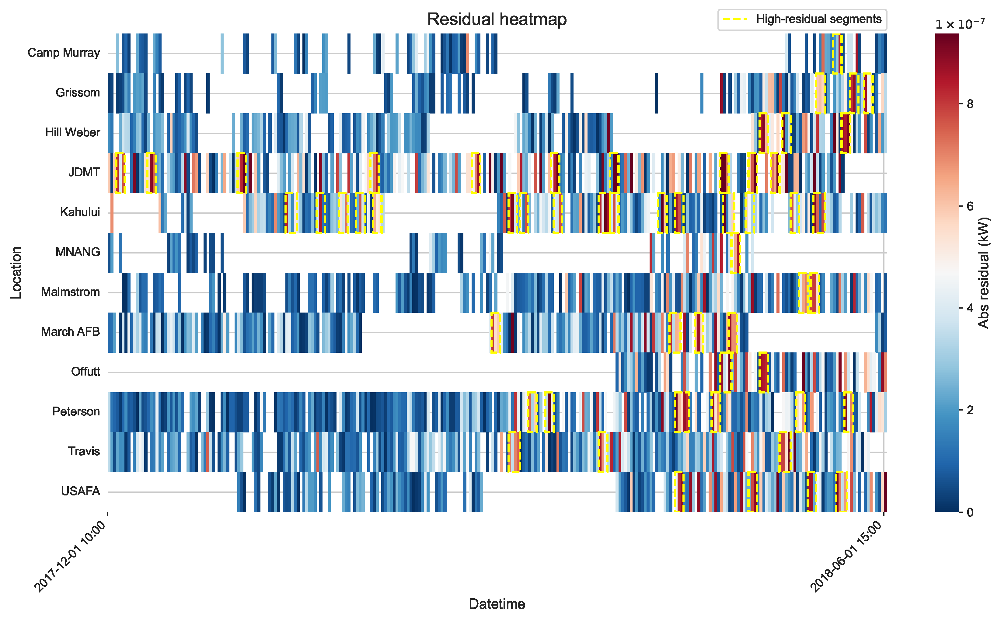
To assess the generative accuracy of GRAIL in reconstructing incomplete photovoltaic sequences, Figure 6 presents a sequence-tile residual heatmap. Each row in the heatmap corresponds to a PV site and each column represents an hourly timestep, with the color encoding the absolute difference between observed and reconstructed power values. The residuals are predominantly concentrated in the deep-blue region, indicating that the generation module in GRAIL consistently captures the underlying temporal dynamics of PV output with high precision. For example, sites such as Camp Murray, Hill Weber, and Malmstrom display uniformly low reconstruction errors across all timestamps, demonstrating the model’s ability to capture site-specific PV power dynamics with high consistency. Although locations such as JDMT and Kahului exhibit more frequent and longer high-residual segments, as highlighted by the dashed yellow boxes in Figure 6, these deviations are temporally localized and spatially confined. This pattern suggests that the reconstruction errors are likely induced by meteorological disturbances rather than a systematic model bias. Moreover, GRAIL maintains temporal stability across the entire analysis horizon, with no observable drift or cumulative degradation in reconstruction performance. This stability underscores the model’s robustness in maintaining sequence integrity over time. Finally, the lack of significant residual concentrations at any single site demonstrates GRAIL’s capability to generalize across heterogeneous locations.

In addition, We also evaluate the clustering outcome of GRAIL through an analysis of the temporal power profiles associated with each cluster. Figure 7 visualizes the average hourly photovoltaic power output between 10:00 and 15:00 for the identified groups. The resulting partition reveals two clearly distinct clusters that correspond to low-generation and high-generation scenarios. Cluster 0 is characterized by a suppressed generation profile, with its output remaining consistently below 4.5 kW. The average output begins at 4.1 kW at 10:00 and declines to 3.3 kW by 15:00. This flat trajectory is indicative of persistent atmospheric attenuation from conditions such as overcast skies or heavy cloud cover. In contrast, Cluster 1 follows a distinct bell-shaped generation curve characteristic of clear-sky conditions. Its power output starts at 9.5 kW, peaks at 13.5 kW around solar noon, and gradually declines to 11.5 kW. The generation amplitude of this cluster is approximately three times that of Cluster 0, which suggests optimal irradiance-to-power conversion efficiency. The distinct separation between the two profiles highlights the model’s capacity to preserve salient structural patterns during the generation and clustering processes. Furthermore, the hour-to-hour profiles within each cluster are nearly parallel, a feature that reflects low intra-cluster variability and high internal consistency. This visual observation aligns with the elevated silhouette scores from Section 3.4 and confirms that GRAIL produces cluster assignments that are both geometrically compact and physically meaningful.

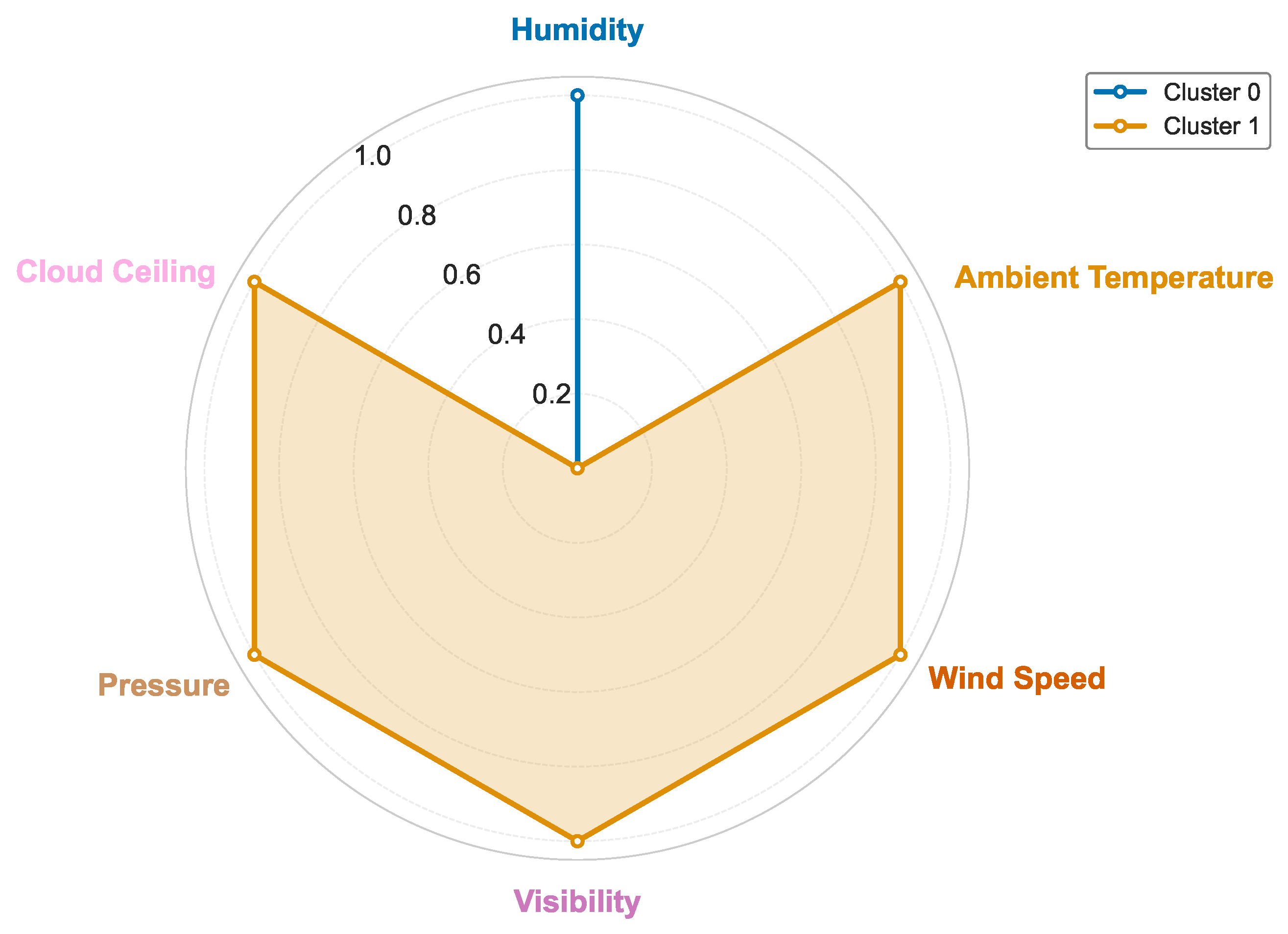
Furthermore, we analyzed the average environmental profiles associated with each cluster. Figure 8 presents a radar plot that contrasts six key meteorological indicators, which are normalized to the $[0,1]$ range for comparability. The two clusters display remarkably divergent environmental characteristics. Cluster 0, indicated by the blue trace, is predominantly characterized by high relative humidity, a condition representative of overcast or saturated settings that attenuate incoming solar radiation and inhibit photovoltaic performance. In contrast, Cluster 1, indicated by the orange trace, exhibits high normalized scores across ambient temperature, wind speed, visibility, surface pressure, and cloud ceiling. These indicators correspond to clear-sky, dry, high-pressure conditions that are conducive to maximized solar insolation. The complementary environmental properties of the two clusters are consistent with their power generation profiles, which show a difference of approximately 9 kW. As evidenced by Figure 7, Cluster 1 captures high-yield daytime windows, while Cluster 0 represents weather-degraded, low-output periods. These clear meteorological distinctions underscore the semantic validity of the clustering produced by the GRAIL framework.

Figure 9 illustrates the convergence behavior of GRAIL’s alternating optimization, with key clustering metrics stabilizing rapidly. The silhouette score shows a steep ascent from 0.13 at iteration 2 to over 0.9 by iteration 4, after which it saturates. This early stabilization indicates that the latent space quickly organizes into compact, well-separated clusters. A comparable trend is observed in the Calinski-Harabasz index, which rises by three orders of magnitude between iterations 5 and 7, suggesting a continued refinement of inter-cluster dispersion even after the initial structure is formed. Inversely, the Davies-Bouldin index exhibits a steady decay, falling below 0.05 by iteration 6, which corroborates the reduction in cluster overlap. Other metrics provide further insight into the training dynamics. The normalized entropy experiences an abrupt increase at iteration 3 and remains at its theoretical maximum, indicating that the sample distribution across clusters becomes balanced early and remains stable. Concurrently, the autoencoder’s reconstruction error remains nearly constant during the initial iterations and only begins to decrease after iteration 5. This delay suggests a strategic shift in the model’s learning process. Once the global cluster geometry stabilizes, GRAIL reallocates its capacity toward refining the localized reconstruction of data, improving generation quality without compromising structural clarity. These patterns demonstrate the computational efficiency of GRAIL. The framework achieves convergence within approximately six outer iterations, dramatically reducing the training cost compared to typical deep clustering models. This accelerated optimization not only improves scalability but also enhances the model’s responsiveness for real-world settings where training budgets may be limited.

The alternating optimization process converges to a stable clustering partition. As shown in Figure 9, once the convergence curves reach a plateau, subsequent outer iterations consistently produce the same partition. To formalize this, we let ${\mathbf{c}}^{\left(t\right)}$ denote the cluster labels and $k^{\left(t\right)}$ be the number of non-noise clusters at outer iteration t. We observe that after the metric curves flatten, which typically occurs within six outer iterations in our experiments, the value of $k^{\left(t\right)}$ becomes constant, and no further cluster merges or splits occur. The stability of the final cluster count is further reinforced by the properties of the clustering algorithm. Because the HDBSCAN configuration is selected from a stability plateau of the min_cluster_size hyperparameter, small perturbations to this value yield the same number of clusters at convergence, indicating robustness. The subsequent k-NN refinement step assigns labels only to points previously marked as noise and does not alter the set of non-noise clusters. Taken together, these observations confirm the within-run stability of both the cluster assignments and the number of clusters produced by the framework.

4. Conclusions

This study introduces GRAIL, a unified framework that integrates cluster-aware data generation, latent feature representation, and adaptive clustering for partitioning real-world distributed photovoltaic data. Distinct from conventional clustering pipelines, GRAIL employs a feedback-driven architecture in which data generation and cluster assignments mutually inform each other, leading to semantically coherent and geometrically discriminative clusters. Through comprehensive experiments, GRAIL consistently outperforms classical methods, deep embedded variants, and other hybrid approaches, achieving state-of-the-art results across multiple evaluation metrics. Beyond its superior accuracy, the framework is computationally efficient. The training procedure converges rapidly within approximately six outer iterations, a significant reduction in computational overhead compared to traditional deep learning models that often require hundreds of epochs. Furthermore, our in-depth analysis reveals that GRAIL exhibits strong physical interpretability, as it successfully detects distinct, weather-driven behaviors from unsupervised spatiotemporal photovoltaic data.

Despite the framework’s strong performance in handling severe data missingness and its rapid convergence, several limitations of this study motivate future work. First, our evaluation relies on a single multi-site dataset over a fixed time window. Although GRAIL’s unsupervised, mask-aware, and density-adaptive design suggests strong potential for portability, broader validation across larger and more diverse PV fleets, spanning varied climates and longer operational horizons, is required to formally quantify its generalization capabilities. Second, while GRAIL is designed to be robust to missing data, it has not been stress-tested against systematic or adversarial corruptions. Potential failure modes, such as large, structured corruptions or slow sensor calibration drift, have not yet been explored. Therefore, we bound the current claims to non-adversarial settings. Future work will directly address this by incorporating several robustness-enhancing features, including contamination-aware training, the use of robust objective functions for reconstruction, and the development of online monitors for outliers and data drift. Furthermore, this study deliberately focuses on an LSTM generator and a benchmark of clustering methods, deferring comparisons to computationally intensive Transformers or forecasting-centric graph networks. Our approach is tailored for unsupervised clustering with missing data, a distinct task from supervised forecasting. Building on this foundation, future work explores these advanced architectures. This includes developing Transformer-based generators to quantify performance trade-offs, integrating spatiotemporal graph priors to leverage richer structural information, and investigating alternative paradigms such as fuzzy clustering to enable soft scenario assignments. Moreover, the framework intentionally avoids direct irradiance inputs to remain robust in common scenarios where such measurements are unavailable or unreliable. We do not claim superiority over irradiance-based pipelines when high-quality irradiance is present. In data-rich deployments, we will quantify the benefit of irradiance via a with-vs-without sensitivity analysis and extend the model to a multimodal conditioning scheme that fuses high-quality irradiance, satellite imagery, and sky-camera signals while preserving mask-aware training. Finally, future research will address practical deployment considerations. This includes formally reporting the computational cost and scalability of GRAIL on large PV fleets and documenting its interoperability with SCADA and forecasting systems. The goal is to develop stable interfaces that expose cluster identifiers and compact state descriptors for direct integration into operational pipelines.