Estimation of Chlorophyll and Water Content in Maize Leaves Under Drought Stress Based on VIS/NIR Spectroscopy

Abstract

Maize (Zea mays) is a key crop, with its growth impacted by drought stress. Accurate, non-destructive assessment of drought severity is crucial for precision agriculture. VIS/NIR reflectance spectroscopy is widely used for estimating plant parameters and detecting stress. However, the relationship between key parameters—such as chlorophyll and water content—and VIS/NIR spectra under drought conditions in maize remains unclear, lacking comprehensive models and validation. This study aims to develop a non-destructive and accurate method for predicting chlorophyll and water content in maize leaves under drought stress using VIS/NIR spectroscopy. Specifically, maize leaf reflectance spectra were collected under varying drought stress conditions, and the effects of different spectral preprocessing methods, dimensionality reduction techniques, and machine learning algorithms were evaluated. An optimal data processing pipeline was systematically established and deployed on an edge computing unit to enable rapid, non-destructive prediction of chlorophyll and water content in maize leaves. The experimental results demonstrated that the combination of stepwise regression (SR) for feature selection and a stacking regression model achieved the best performance for chlorophyll content prediction (${\mathrm{R}}_{\mathrm{p}}^2$ = 0.8740, RMSE_p = 0.2768). For leaf water content prediction, random forest (RF) feature selection combined with a stacking model yielded the highest accuracy (${\mathrm{R}}_{\mathrm{p}}^2$ = 0.7626, RMSE_p = 4.12%). This study confirms the effectiveness and potential of integrating VIS/NIR spectroscopy with machine learning algorithms for monitoring drought stress in maize, offering a valuable theoretical foundation and practical reference for non-destructive crop physiological monitoring in precision agriculture.

1. Introduction

Maize (Zea mays) is the third most widely consumed cereal crop globally, accounting for over half of the caloric intake from grains worldwide [1]. It plays a vital role in the ever-evolving global agricultural and food systems and serves multiple functions in both industrial and livestock sectors [2]. However, the increasing frequency of extreme weather events, such as drought—driven by global climate change—poses a serious threat to the stability and sustainability of global maize production [3]. Environmental changes present a significant challenge to agriculture’s ability to meet the growing global food demand [4]. Among these challenges, drought stress severely inhibits the growth and development of maize plants, leading to reduced plant height, restricted reproduction, and significant declines in grain yield, with potential yield losses reaching up to 43% [5]. Under drought conditions, plants exhibit a range of physiological responses, such as reduced levels of photosynthetic pigments, including chlorophyll and carotenoids, and stomatal closure to limit water loss through transpiration. These responses result in decreased cellular water content and suppressed growth [6]. Such physiological changes indicate that dynamic variations in leaf chlorophyll and water content can directly reflect a crop’s level of drought stress and tolerance. Therefore, these parameters serve as crucial indicators for assessing plant health and performance under drought conditions.

Traditional methods for measuring chlorophyll and water content, such as the Acetone Extraction Method, Dimethyl Sulfoxide (DMSO) Extraction Method, and Karl Fischer Titration, offer high accuracy but are often complex, time-consuming, and potentially environmentally hazardous. These limitations make them unsuitable for large-scale field monitoring. Consequently, developing a rapid, accurate, non-destructive, and environmentally friendly method has become a key research focus in modern agricultural production.

In recent years, near-infrared (NIR) spectroscopy has emerged as a prominent research focus for plant physiological assessment due to its outstanding advantages, including rapid measurement, non-destructive sampling, and potential for real-time, online monitoring [7,8]. NIR spectroscopy enables rapid, non-invasive evaluation of plant physiological status by capturing the characteristic absorption spectra of molecular bonds, such as C–H, N–H, and O–H, in the near-infrared region [9,10]. This technology can be employed independently or in combination with specific wavelengths in the visible (VIS) spectrum (400–750 nm) [11]. Compared to other spectral techniques, NIR spectroscopy is more complex due to the presence of broader absorption bands associated with combination and overtone vibrations of C–H, N–H, and O–H bonds in the near-infrared range [7,12]. These spectral characteristics have provided feasible pathways for the rapid prediction of plant physiological parameters [13,14,15,16]. However, NIR spectral data often contain substantial redundancy, complex spectral fingerprints, and multiple sources of noise or interference, which limit their direct use for efficient quantitative analysis [17]. Therefore, effectively extracting and utilizing key information embedded in VIS/NIR spectral data remains a critical challenge.

Despite extensive research on spectral preprocessing and feature extraction techniques, refined quantitative inversion of chlorophyll and water content in maize—particularly during the seedling stage under drought stress—remains insufficiently explored. This gap presents a critical limitation for the development of precision agriculture and the effective monitoring of drought stress in maize. Therefore, the development of rapid and accurate methods for chlorophyll and water content estimation, along with a systematic analysis of the performance of different technical combinations, holds significant practical importance and scientific value.

In this study, we propose a non-destructive estimation approach for chlorophyll and water content in maize leaves under drought stress, based on VIS/NIR spectroscopy. Our primary contribution lies in systematically establishing an optimal modeling framework by exploring combinations of various spectral processing and machine learning techniques. The resulting quantitative models describe the relationship between VIS/NIR spectra and physiological parameters under drought conditions and are successfully deployed on edge computing devices to enable rapid, non-invasive prediction in the field.

The objectives of this study are as follows:

(1) To collect VIS/NIR spectra of maize leaves with varying chlorophyll and water content and analyze their spectral variation patterns.

(2) To evaluate the impact of different preprocessing, dimensionality reduction, and regression methods on model performance.

(3) To identify the optimal combination of techniques for accurate prediction.

(4) To validate the performance and generalization ability of the developed portable sensing device.

2. Materials and Methods

2.1. Samples and Experimental Setup

The experiment was conducted in a controlled greenhouse at the College of Agriculture, Guangxi University, using the maize cultivar ‘Zaoshengnuo 808’. Drought stress treatments were applied starting at the four-leaf seedling stage to investigate spectral responses under varying drought conditions. The experimental design included a control group (CK) and three drought stress levels (W1, W2, W3), each with 12 replicates, totaling 48 pots. The control group (CK) was maintained under optimal irrigation with soil moisture at 75% of field capacity (FC). The drought treatments were defined as mild (W1, 60% FC), moderate (W2, 45% FC), and severe (W3, 30% FC). Field capacity refers to the maximum water content retained in soil after excess water has drained. To eliminate rainfall interference, all treatments were performed indoors. Normal irrigation was maintained before the four-leaf stage, after which drought stress was initiated. Soil moisture was monitored daily at 17:00 using a gravimetric method, and water was replenished as needed to maintain target levels. Leaf sampling was conducted at 9:00 a.m. on days 3, 6, and 9 after stress initiation. For each treatment, four maize plants were randomly selected, and three topmost leaves per plant were collected. The leaves were cut into two sections using sterilized scissors, immediately sealed in specimen bags, and transported to the laboratory for further analysis.

2.2. Data Collection

A portable CI-710 fiber-optic spectrometer (CID Bio-Science, Camas, WA, USA) was used to collect VIS/NIR reflectance spectra of the maize leaves. The device has a spectral range of 400–1000 nm, an optical resolution of 1.5 nm, and a measurement chamber diameter of 7.6 mm. To minimize spectral drift, the spectrometer was preheated for 10 min at a stable room temperature of 26 °C. Instrument calibration was performed using a white reference panel aligned with the light source for baseline correction. During spectral measurement, freshly excised maize leaves were immediately placed in the leaf clip, and reflectance spectra were recorded at multiple positions along the leaf surface. Each leaf was measured five times consecutively, and the average spectrum was used as the representative data for that leaf. In total, 288 spectral samples were obtained. Due to high noise levels below 450 nm and above 970 nm, only the spectral range of 450–970 nm was retained for subsequent analysis.

After spectral data collection, the chlorophyll content in the maize leaves was determined following the Lichtenthaler–Wellburn method [18]. Approximately 0.1 g of leaf tissue (excluding the veins) was quickly excised, ground, and immediately transferred into a test tube containing 25 mL of a mixed solvent of acetone and absolute ethanol (v/v = 2:1). The samples were extracted in the dark at room temperature for 24 h until complete decolorization of the leaf tissue. The resulting extract was transferred to a cuvette using a micropipette, and absorbance was measured at 663 nm and 645 nm using a UV–visible spectrophotometer (UV1800, Shimadzu Corporation, Kyoto, Japan). Chlorophyll content (mg/cm²) was calculated using the following equation:

Chlorophyll content(mg/cm²) = (8.02 × OD₆₆₃ + 20.21 × OD₆₄₅) × V/(S × 1000),

(1)

where V represents the volume of the extraction solution (mL) and S is the sampled leaf area (cm²).

Relative water content (RWC) is a reliable indicator of leaf physiological status under varying water conditions and is widely used to assess plant water status [19]. After removing the veins, the leaf samples were immediately weighed to obtain the fresh weight (WF) using an electronic balance with 0.001 g precision. The samples were then soaked in distilled water for 2 h to achieve full turgidity. After gently blotting surface moisture, the turgid weight (WS) was recorded. To obtain the dry weight (WD), the leaves were first inactivated in a 105 °C oven for 30 min to halt metabolic activity, followed by continuous drying at 80 °C until a constant weight was reached (Figure 1). The relative water content (RWC) was calculated using the following equation:

RWC(%) = (W_F − W_D)/(W_S − W_D) × 100%,

(2)

where W_F, W_D, and W_S are fresh weight, dry weight, and turgid weight, respectively, expressed in grams (g). The resulting RWC was expressed as a percentage (%).

2.3. Spectral Data Processing

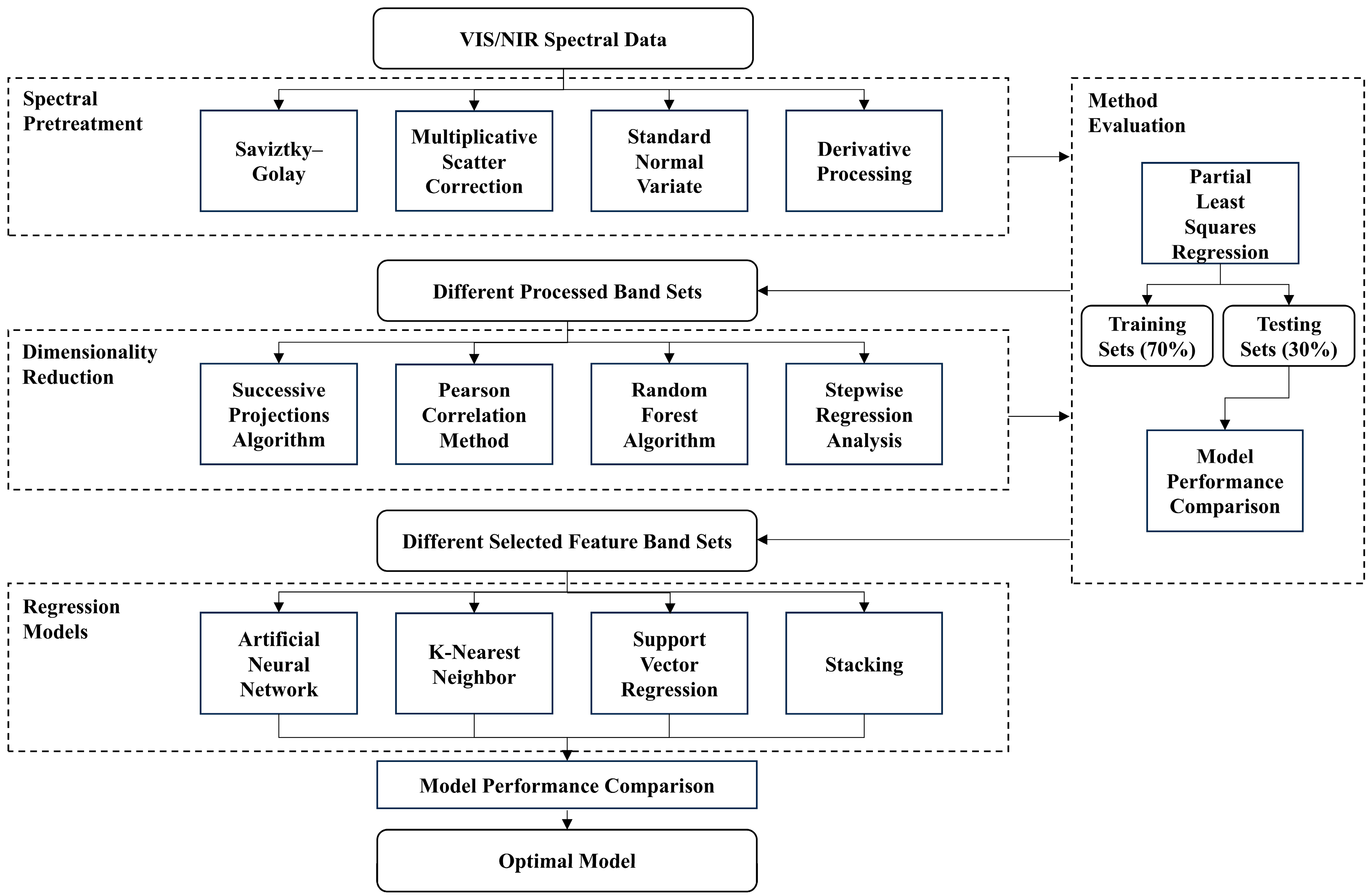
In this study, spectral data were first preprocessed to reduce noise and variability. Dimensionality reduction was then performed by extracting characteristic wavelengths to minimize data redundancy. Subsequently, regression models were developed using machine learning algorithms to establish the relationship between spectral reflectance features and maize leaf chlorophyll and water content. To achieve optimal prediction accuracy and model robustness, various combinations of preprocessing methods, feature reduction techniques, and regression algorithms were systematically evaluated. The best-performing model configuration was identified based on a comprehensive performance comparison (Figure 2).

2.3.1. Data Preprocessing and Dimensionality Reduction

Raw spectral data contain essential information reflecting the characteristics of the samples; however, they are also affected by various interference factors, such as stray light, baseline drift, and random noise. These factors can obscure the true signal and significantly impair the performance of subsequent predictive models. Therefore, effective data preprocessing is not only theoretically necessary but also a critical step in improving model accuracy in practical applications.

To mitigate the impact of random noise present in the acquired spectral data, the Savitzky–Golay (SG) smoothing algorithm was employed in this study [20]. This method fits a polynomial to the data points within a moving window using the least squares approach. It effectively suppresses random noise while preserving the original spectral features of a sample as much as possible in real-world scenarios.

Spectral data acquisition is often affected by pronounced scattering effects, which typically manifest as fluctuations and distortions in spectral intensity during practical applications. To correct for these distortions, this study employed two methods: Multiplicative Scatter Correction (MSC) and Standard Normal Variate (SNV) transformation [21,22].

In addition, spectral baseline drift is unavoidable during actual measurements. First derivative (FD) preprocessing can effectively reduce the negative effects of baseline shifts, improve data resolution, and highlight subtle spectral features.

Considering the high dimensionality and strong inter-band correlation inherent in VIS/NIR spectral data, a key challenge lies in reducing redundancy while preserving informative spectral features. In this study, preprocessing methods were selected and arranged based on their complementary methodological principles—each addressing spectral enhancement from a different perspective, including noise suppression, scattering and baseline drift removal, and resolution improvement. To avoid information loss or over-processing, all methods were applied independently rather than sequentially, with no combined transformations, ensuring that each could contribute uniquely without introducing mutual redundancy.

For subsequent feature selection and model construction, this study employed four dimensionality reduction methods: the successive projections algorithm (SPA) [23], the Pearson correlation coefficient method [24], random forest (RF) [25,26], and stepwise regression analysis (SR) [27]. These methods were intentionally chosen for their methodological complementarity—SPA focuses on removing multicollinearity, Pearson correlation targets linear relevance, RF captures nonlinear interactions, and SR emphasizes model parsimony—thereby improving the efficiency and accuracy of predictive modeling.

2.3.2. Regression Model

After dimensionality reduction and feature band extraction, this study employed several machine learning models to develop regression models for predicting chlorophyll and water content in maize leaves and conducted a comparative analysis of their performance. The models included partial least squares regression (PLSR) [28], an artificial neural network (ANN) [29], k-nearest neighbor (KNN) [30], support vector regression (SVR) [31], and a stacking ensemble learning method [32]. In the stacking framework, the ANN, KNN, and SVR models were used as base learners, while linear regression served as the meta-learner.

2.4. Data Partition and Model Evaluation

This study used the coefficient of determination (${\mathrm{R}}^2$) and root mean square error (RMSE) to evaluate model performance. ${\mathrm{R}}^2$ indicates the goodness of fit; values closer to 1 indicate a better fit. RMSE reflects average prediction error; lower values indicate higher accuracy. ${\mathrm{R}}_{\mathrm{c}}^2$, RMSE_c and ${\mathrm{R}}_{\mathrm{p}}^2$, RMSE_p refer to the training and testing sets, respectively. ${\mathrm{R}}_{\mathrm{t}}^2$, ${\mathrm{RMSE}}_{\mathrm{t}}$ and ${\mathrm{R}}_{\mathrm{v}}^2$, RMSE_v refer to the training and validation subsets in cross-validation. To objectively assess generalization ability, the dataset was randomly split into training and test sets at a 7:3 ratio (

Table 1. Statistical analysis of chlorophyll content and water content of maize leaves.

Inversion Target	Sample	Number	Max	Min	Mean	Standard Deviation
Chlorophyll Content (mg/g)	Training set samples	201	5.3889	1.4506	3.6406	0.8144
	Testing set samples	87	5.2773	1.8251	3.7057	0.7849
	All samples	288	5.3889	1.4506	3.6444	0.8046
Relative Water Content (%)	Training set samples	201	98.54	46.78	77.42	9.47
	Testing set samples	87	93.40	53.94	77.62	7.88
	All samples	288	98.54	46.78	77.31	8.89

). Five-fold cross-validation was applied within the training set to optimize model structure and parameters, with the average validation performance used to select the optimal configuration. Final model evaluation was based on predictions from the held-out test set.

As shown in Table 1, the chlorophyll content in the maize leaves ranged from 1.45 to 5.39 mg/g, and the relative water content varied from 46.78% to 98.54%. The mean chlorophyll values were 3.64 mg/g (SD = 0.81 mg/g) in the training set and 3.71 mg/g (SD = 0.783.71 mg/g) in the testing set, while the relative water content averaged 77.42% (SD = 9.47%) and 77.62% (SD = 7.88%), respectively. The close agreement between the means and standard deviations demonstrates that both datasets are well balanced and highly consistent. Moreover, the wide value ranges ensure adequate coverage of physiological variation, while the similarity between the training and testing subsets indicates that the data partitioning was appropriate for model development and evaluation. The standard deviation (SD) was calculated as follows:

$$\mathrm{SD} =\sqrt{{\displaystyle \frac{1}{n-1}}{\sum }_{i = 1}^n(x_i-\overline{x}{)}^2},$$

(3)

where n represents the number of observations, $x_i$ is the value of the ith observation, and $\overline{x}$ denotes the sample mean. The denominator (n − 1) is applied to obtain an unbiased estimate of the population standard deviation.

3. Results

3.1. Maize Leaf Responses and Spectral Characteristics Under Drought Stress

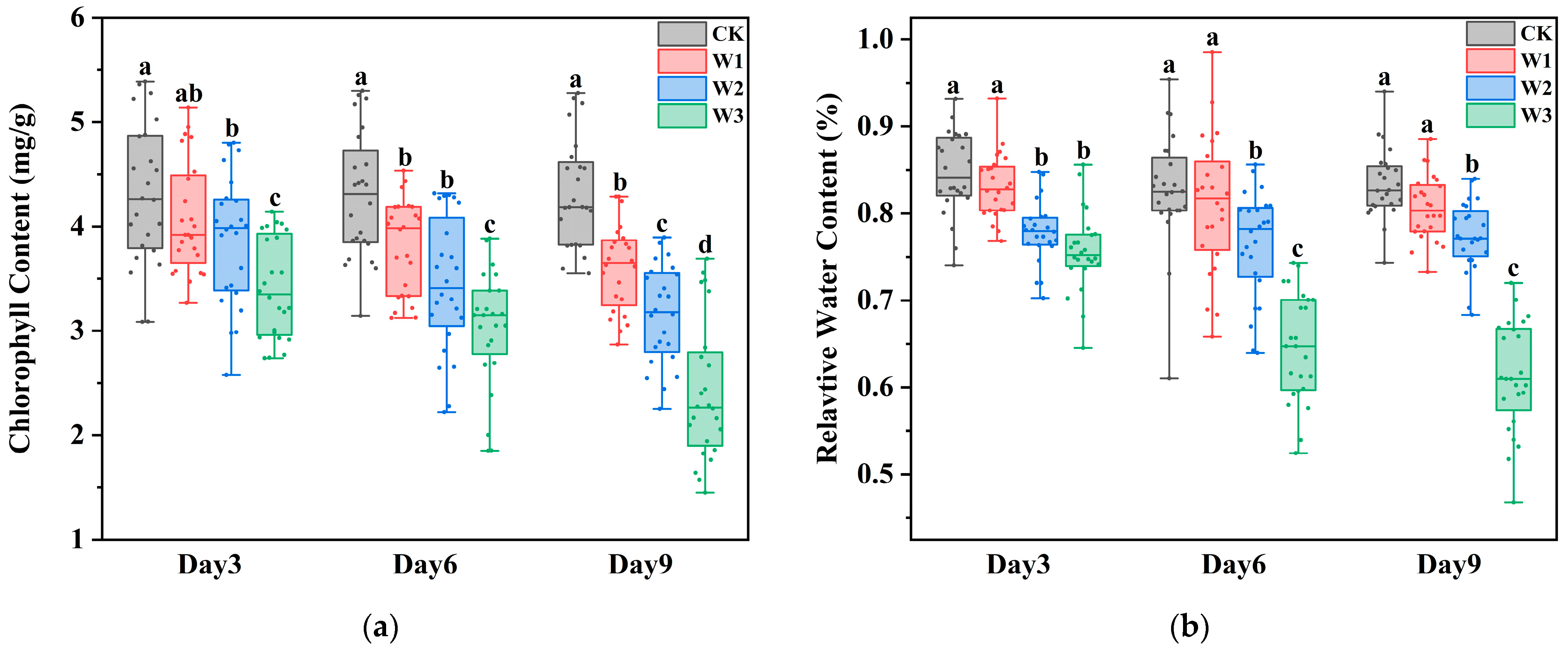
Under different drought stress conditions, both the chlorophyll content and the leaf water content in maize showed a significant decreasing trend (Figure 3). The chlorophyll content declined progressively with increasing drought intensity and duration, with statistically significant differences observed among the treatments (p < 0.05), likely due to inhibited water and nutrient uptake affecting chlorophyll synthesis. The significance threshold (p < 0.05) was determined from the p-value of the F-test in the one-way ANOVA, which assesses whether there are overall differences among treatment means. Similarly, the water content decreased with prolonged and intensified stress: it declined slowly under mild drought, dropped rapidly during the first three days under moderate drought before stabilizing, and decreased sharply within the first six days under severe drought. Differences in water content among the treatments were also significant over time (p < 0.05). These results indicate that chlorophyll and water content are effective indicators for assessing maize responses to drought stress.

Due to the strong correlation between maize leaf reflectance spectra and both chlorophyll and water content, this relationship forms the theoretical basis for using spectral techniques to assess leaf physiological status. This study analyzed the spectral characteristics of maize leaves under varying levels of drought stress. In the visible region, the “green peak” (~550 nm) and “red edge” (680–750 nm) are primarily influenced by chlorophyll, with strong absorption at ~450 nm (blue) and ~680 nm (red) and higher reflectance in the green region. The red edge, characterized by a rapid increase in reflectance, indicates chlorophyll levels and plant health. In the near-infrared region (700–1300 nm), reflectance is influenced by internal leaf structure and water content, with notable water absorption at 970, 1200, and 1450 nm. As shown in Figure 4, average spectral reflectance increased with drought severity, with a consistent trend of W3 > W2 > W1 > CK across the 450–970 nm range, indicating significant spectral response to drought. Overall, variations in chlorophyll and water content can be effectively captured through spectral reflectance, demonstrating the feasibility and practical value of spectral inversion for drought stress monitoring in maize.

3.2. Preprocessing of Leaf Spectral Data

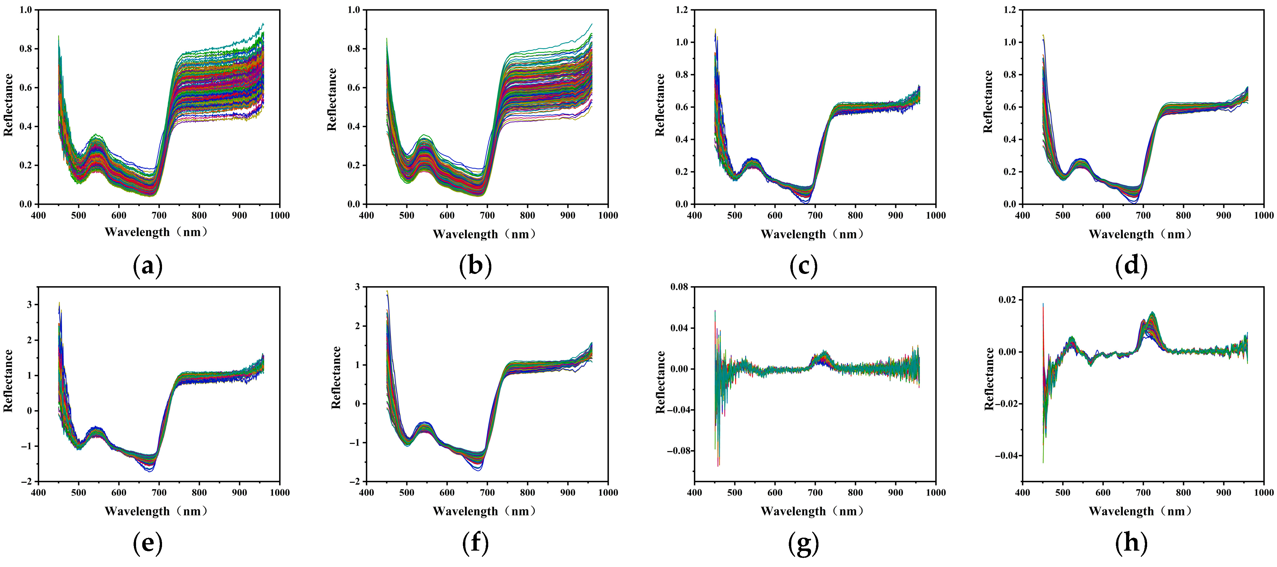
The performance of preprocessing methods is related to data distribution and algorithm parameters. Therefore, this study compared the performance of different preprocessing methods to identify the most suitable spectral preprocessing technique for the research. The methods adopted in this study include Savitzky–Golay smoothing (SG), multiplicative scatter correction (MSC), standard normal variate (SNV), and first derivative (FD), as well as three combined methods involving SG: SG + MSC, SG + SNV, and SG + FD. These preprocessing techniques were respectively applied to the raw spectral data and combined with partial least squares regression (PLSR) to construct models for predicting chlorophyll and water content. The number of principal components was determined through cross-validation, and model performance was evaluated on the test set (see

Table 2. Predictive performance of different pretreatment spectra versus original spectra for chlorophyll content and water content.

Component	Preprocessing Methods	LVs	Cross-Validation Training Set		Cross-Validation Validation Set		Test Set
			${\mathbf{R}}_{\mathbf{t}}^2$	RMSEt	${\mathbf{R}}_{\mathbf{v}}^2$	RMSEv	${\mathbf{R}}_{\mathbf{p}}^2$	RMSEp
Chlorophyll Content (mg/g)	Original	9	0.9206	0.2307	0.8114	0.3482	0.8099	0.3275
	SG	5	0.8217	0.3460	0.7960	0.3585	0.8129	0.3249
	MSC	7	0.8117	0.3558	0.5796	0.5168	0.6653	0.4346
	SNV	6	0.7389	0.4180	0.5946	0.5141	0.6298	0.4570
	FD	2	0.7970	0.3662	0.5822	0.5013	0.6586	0.4389
	SG + MSC	7	0.6838	0.4614	0.5509	0.5387	0.5935	0.4789
	SG + SNV	6	0.6167	0.5080	0.5734	0.5287	0.5681	0.4936
	SG + FD	1	0.6619	0.4766	0.6094	0.4986	0.5017	0.5302
Relative Water Content (%)	Original	10	0.9195	2.42	0.7462	4.24	0.7795	4.75
	SG	13	0.8727	2.79	0.7189	4.44	0.7815	4.64
	MSC	9	0.8989	2.71	0.6349	5.05	0.6755	5.66
	SNV	10	0.9115	2.54	0.6390	5.02	0.6840	5.58
	FD	3	0.8504	3.30	0.6275	5.13	0.7023	5.42
	SG + MSC	12	0.8910	2.82	0.5837	5.42	0.6186	7.09
	SG + SNV	13	0.8146	3.67	0.5476	5.65	0.5186	6.89
	SG + FD	5	0.8852	2.89	0.6631	4.88	0.7169	5.28

Bold values indicate the best results.

).

Compared with the raw spectra (Figure 5a), all preprocessing methods except SG resulted in decreased prediction accuracy for both the chlorophyll content and water content. SG demonstrated the best performance among all methods. As shown in Figure 5b, SG effectively smoothed the spectral curves while preserving the key spectral features and significantly reducing high-frequency noise. MSC and SNV also maintained the overall spectral shape (Figure 5c,e), but the distinction in key regions, such as the green peak and near-infrared band, was weakened. However, the combined preprocessing methods SG + MSC and SG + SNV (Figure 5d,f) did not improve the performance compared with MSC and SNV alone, and in some cases even weakened the predictive capacity, suggesting no additional benefit from combining these methods. In addition, SNV performed centering and standardization on each spectrum, which helped eliminate baseline shifts and scale effects.

Although FD enhanced certain spectral features, it also amplified noise, resulting in overlapping and unclear peak and valley signals (Figure 5g). However, when SG smoothing was applied before FD (SG + FD), the noise was effectively suppressed and the spectral features became more distinct (Figure 5h), showing two prominent peaks around 525 nm and 750 nm and a valley near 550 nm.

Based on the comprehensive comparison, SG preprocessing was identified as the optimal method for building models to predict the chlorophyll and water content in maize leaves in this study.

3.3. Dimensionality Reduction and Feature Bands Selection

To reduce the dimensionality of spectral data, minimize redundancy, and improve model performance, four feature wavelength selection algorithms were applied to the preprocessed spectral dataset: successive projections algorithm (SPA), Pearson correlation, random forest (RF), and stepwise regression (SR). Each method was used in combination with linear regression to evaluate its effectiveness for predicting chlorophyll and leaf water content.

3.3.1. SPA

The number of feature wavelengths selected by the successive projections algorithm (SPA) was determined based on the number of variables corresponding to the minimum root mean square error (RMSE) observed during model training.

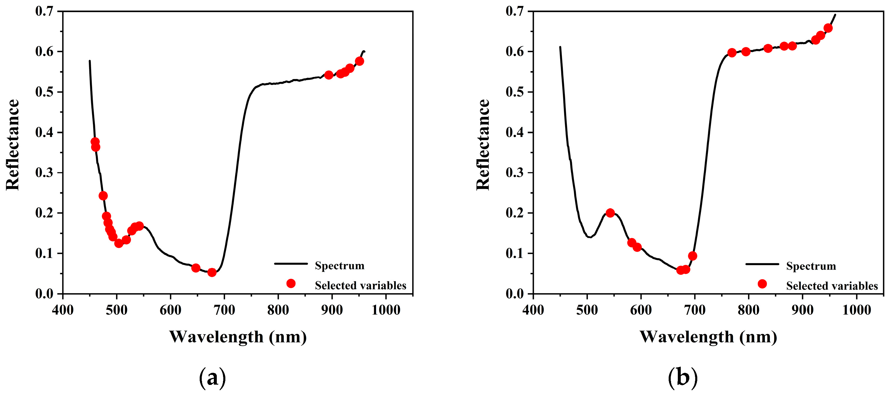
For chlorophyll content estimation, the SPA selected 20 feature wavelengths, accounting for 3.9% of the total spectral bands. For leaf water content estimation, 14 wavelengths were selected, representing 2.7% of the total.

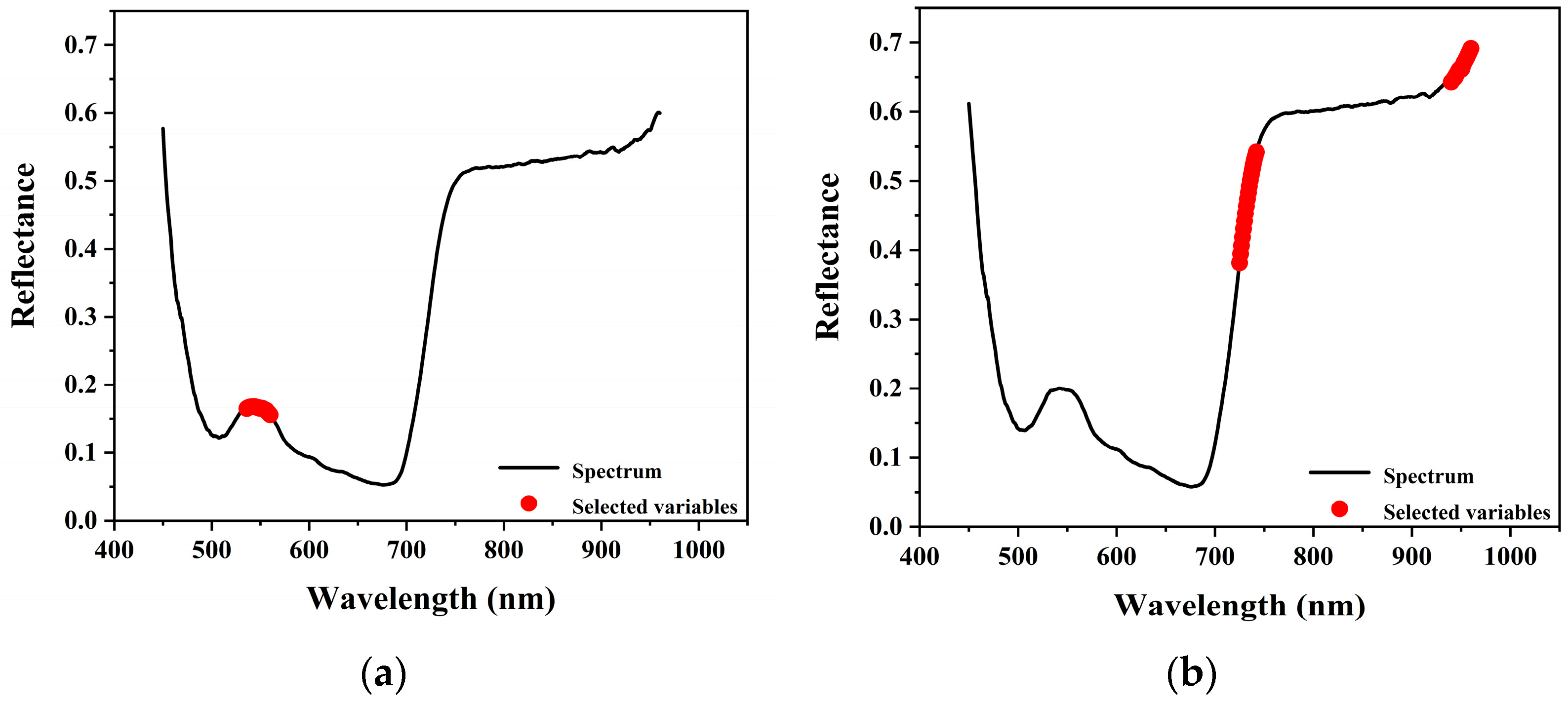
As shown in Figure 6, the relationship between the number of selected wavelengths and RMSE was used to determine the optimal subset size. The distribution of selected wavelengths is illustrated in Figure 7.

3.3.2. Pearson Correlation Method

The Pearson correlation method was used to calculate the correlation coefficients between the spectral reflectance and the target variables, including the chlorophyll content and water content.

The chlorophyll content exhibited a strong negative correlation with reflectance. Wavelengths with absolute correlation coefficients greater than 0.8 were primarily located in the green peak region (516–623 nm) and the red-edge region (712–729 nm), with the strongest correlation (|R| = 0.8968) observed at 546 nm. Similarly, the water content also showed negative correlations with reflectance, and stronger correlations were generally observed in the near-infrared region. The highest absolute correlation (|R| = 0.7913) was found at 732 nm. The correlation plots are presented in Figure 8.

To determine the optimal number of feature wavelengths, all wavelengths were ranked by the absolute values of their correlation coefficients. Linear regression models were then constructed using subsets of the top 5, 10, 15, 20, 25, 30, 35, and 40 wavelengths. Based on the test set results, the top 25 wavelengths were selected for chlorophyll prediction and the top 35 for water content prediction. The final wavelength distributions are shown in Figure 9.

3.3.3. RF

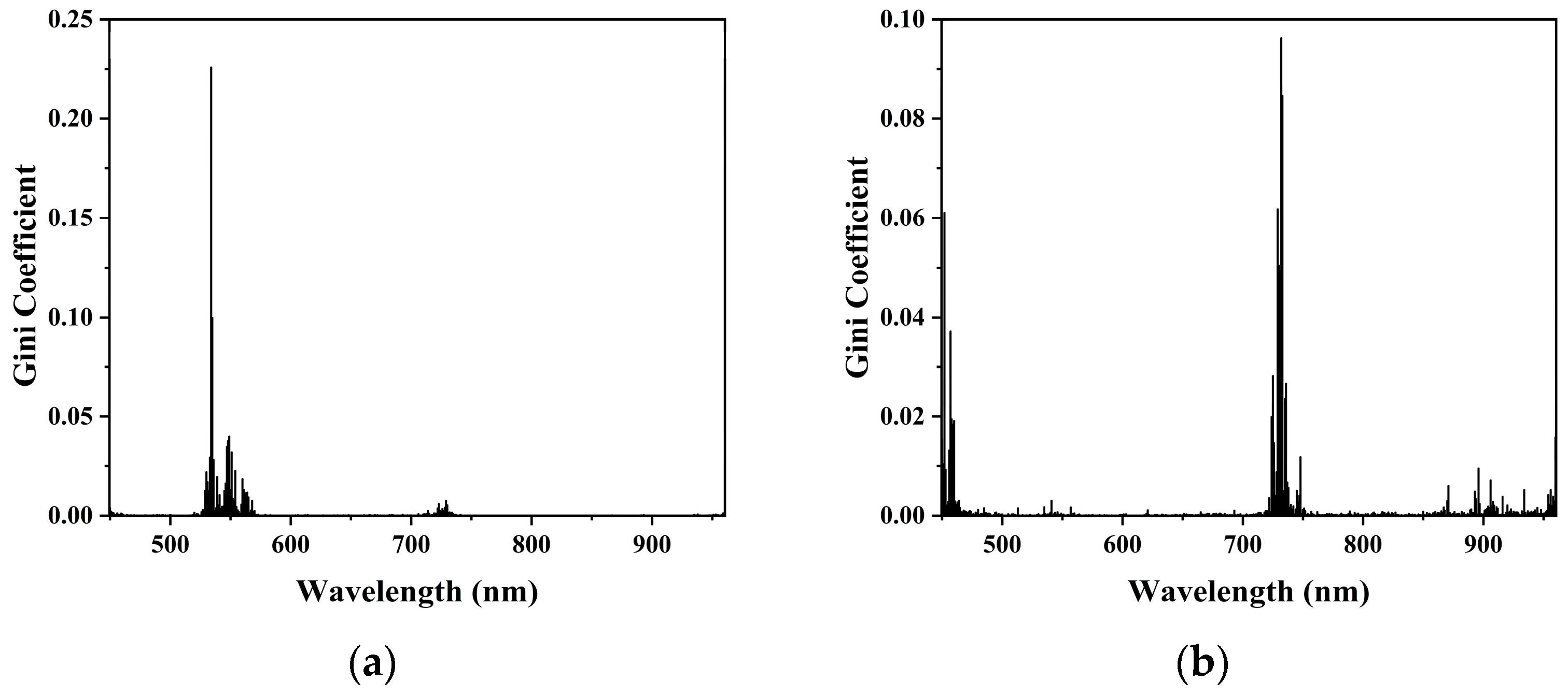
The importance of each wavelength in predicting chlorophyll and water content was evaluated using Gini coefficients obtained from the random forest (RF) algorithm.

For chlorophyll prediction within the 450–970 nm range, the most important wavelength was 534 nm, with a Gini coefficient of 0.2259. For water content prediction, high-importance wavelengths were mainly concentrated in the 400–500 nm and 700–750 nm ranges. The most significant wavelength was 732 nm, with a Gini coefficient of 0.0963. The Gini coefficient distributions are presented in Figure 10.

The wavelengths were ranked in descending order of their Gini importance scores. Subsets of the top 5, 10, 15, 20, 25, 30, 35, and 40 wavelengths were used to construct feature combinations, which were subsequently integrated into linear regression models. Based on the test set results, the top 20 wavelengths were selected for both chlorophyll and water content prediction. The selected bands are shown in Figure 11.

3.3.4. SR

The stepwise regression (SR) algorithm selected six and five feature wavelengths for chlorophyll and water content prediction, respectively, effectively eliminating 515 and 516 wavelengths from the full spectrum.

The selected wavelengths for chlorophyll prediction were primarily distributed in the green and red absorption regions of the visible spectrum, while those for water content prediction spanned several key regions from the visible to the near-infrared range. These results are visualized in Figure 12.

3.3.5. Comparative Analysis

As shown in

Table 3. Grouping of chlorophyll and water content prediction model input variables.

Inversion Target	Variable Set	Dimensionality Reduction Method	Selected Wavelengths (nm)
Chlorophyll Content (mg/g)	C1	Full spectrum	450–970
	C2	SPA	460, 461, 475, 481, 484, 487, 490, 493, 504, 518, 528, 534, 542, 647, 677, 894, 916, 924, 933, 951
	C3	Pearson correlation method	536, 537, 538, 539, 540, 541, 542, 543, 544, 545, 546, 547, 548, 549, 550, 551, 552, 553, 554, 555, 556, 557, 558, 559, 560
	C4	RF	529, 530, 531, 532, 533, 534, 535, 536, 539, 545, 546, 547, 548, 549, 550, 551, 554, 560, 561, 564
	C5	SR	545, 546, 671, 672, 681, 683
Relative Water Content (%)	W1	Full spectrum	450–970
	W2	SPA	534, 583, 593, 674, 683, 696, 769, 795, 836, 866, 881, 924, 933, 947
	W3	Pearson correlation method	725, 726, 727, 728, 729, 730, 731, 732, 733, 734, 735, 736, 737, 738, 739, 740, 741, 742, 940, 943, 944, 946, 950, 951, 954, 956, 958, 959, 961, 963, 964, 965, 966, 967, 968
	W4	RF	450, 451, 452, 456, 457, 458, 459, 560, 724, 725, 726, 729, 730, 731, 732, 733, 735, 736, 748, 970
	W5	SR	540, 701, 726, 860, 914

, the four feature selection methods demonstrated notable differences in their extraction capabilities and application suitability.

The SPA method effectively reduced spectral redundancy by eliminating multicollinearity among the variables. The selected wavelengths were primarily distributed in the blue–green range, red absorption region, and near-infrared water absorption bands, all of which are physiologically sensitive regions. However, since the SPA focuses solely on inter-variable redundancy, it does not explicitly consider the direct relevance between features and target parameters, which may lead to the omission of important information.

The Pearson correlation method selected feature wavelengths mainly concentrated in the green peak region for chlorophyll prediction and in the red-edge and near-infrared regions for water content prediction. This method is simple to implement and computationally efficient, making it suitable for cases with strong linear relationships. However, it does not account for interactions among variables, which may result in feature redundancy and limit improvements in model performance.

The random forest-based Gini importance method selected wavelengths distributed across the green peak and red-edge transition zones, both of which are physiologically relevant for chlorophyll concentration and plant stress detection. This method outperformed the others in terms of both prediction accuracy and model robustness. It achieved a strong balance between dimensionality reduction and modeling performance, making it particularly suitable for complex inversion tasks involving nonlinear relationships between spectral features and target variables.

The stepwise regression (SR) method retained the fewest feature wavelengths, located in the green peak and red-edge regions—both well-known indicators of chlorophyll content and photosynthetic activity. However, this aggressive dimensionality reduction may result in the loss of critical spectral information, leading to lower prediction accuracy and reduced applicability in practical inversion scenarios.

In terms of predictive performance, models based on the RF method yielded the highest accuracy for both chlorophyll and water content estimation, effectively balancing feature importance and nonlinear variable interactions. The Pearson method remained computationally efficient and suitable for datasets with strong linear correlations, though it introduced a degree of redundancy. The SPA selected highly representative bands and was beneficial for tasks prioritizing variable independence. While SR achieved the greatest reduction in input dimensionality, this may have led to the omission of informative bands; nonetheless, SR remains valuable for applications requiring computational simplicity or strict feature constraints.

Overall, the comparison (see

Table 4. Comparative analysis of using input variable sets selected by different dimensionality reduction methods (C2-C5, W2-W5) directly using the original spectrum (C1, W1).

Inversion Target	Variable Set	Input Variables (% of Original)	${\mathbf{R}}_{\mathbf{c}}^2$	RMSEc	${\mathbf{R}}_{\mathbf{p}}^2$	RMSEp
Chlorophyll Content (mg/g)	C1	511 (100%)	0.8732	0.2890	0.7885	0.3554
	C2	20 (3.9%)	0.8425	0.3216	0.7740	0.3660
	C3	25 (4.9%)	0.8384	0.3157	0.7344	0.3733
	C4	20 (3.9%)	0.8323	0.3318	0.7766	0.3650
	C5	6 (1.2%)	0.8263	0.3378	0.7915	0.3530
Relative Water Content (%)	W1	511 (100%)	0.5939	0.0556	0.3202	0.0679
	W2	14 (2.7%)	0.5338	0.0599	0.3890	0.0668
	W3	35 (6.8%)	0.5500	0.0611	0.2879	0.0736
	W4	20 (3.9%)	0.4727	0.0626	0.3917	0.0694
	W5	5 (1.0%)	0.3723	0.0683	0.3079	0.0696

Bold values indicate the best results.

) indicates that the RF method provided the best balance between model accuracy and wavelength selection effectiveness, making it the preferred choice in this study. The Pearson and SPA methods can serve as complementary tools, particularly in scenarios emphasizing model interpretability or where the number of features must be limited. Although SR showed slightly lower accuracy in some tasks, its strength in compressing input dimensionality is noteworthy, especially for remote sensing applications sensitive to computational complexity or requiring real-time performance.

3.4. Results of Predicting Chlorophyll Content

The feature wavelengths extracted by the SPA, Pearson correlation, RF, and SR methods were used as input variables for four regression models: ANN, SVR, KNN, and stacking. In the stacking model, ANN, SVR, and KNN were used as base learners, and a linear regressor was used as the meta-learner. The hyperparameters to be optimized for each regression method are listed in

Table 5. Hyperparameters to be optimized for each regression method.

Regression Model	Parameters Requiring Optimization
ANN	Number of hidden layer neurons = [(1~50)] Activation function = [‘relu’, ‘tanh’, ‘sigmoid’]
SVR	Kernel function = [‘linear’, ‘poly’, ‘rbf’, ‘sigmoid’] Penalty coefficient = [0.001, 0.01, 0.1, 1, 10, 100, 1000]
KNN	Number of nearest neighbors = [(1~30)]

. The optimal parameters were determined via cross-validation, and model performance was evaluated on the test set to identify the best inversion models for chlorophyll and water content.

The model performance for chlorophyll content prediction is shown in

Table 6. Inversion of chlorophyll content of maize leaves by different feature selection methods and regression models.

Feature Selection Methods	Regression Model	Cross-Validation Training Set		Cross-Validation Set		Test Set
		${\mathbf{R}}_{\mathbf{t}}^2$	RMSEt (mg/g)	${\mathbf{R}}_{\mathbf{v}}^2$	RMSEv (mg/g)	${\mathbf{R}}_{\mathbf{p}}^2$	RMSEp (mg/g)
All Spectrum	ANN	0.8970	0.2603	0.8405	0.3194	0.8238	0.3274
	SVR	0.9056	0.2790	0.8205	0.3360	0.8625	0.2893
	KNN	0.8895	0.2691	0.8022	0.3493	0.7968	0.3516
	Stacking	0.9149	0.2364	0.8414	0.3133	0.8683	0.2831
SPA	ANN	0.8597	0.2989	0.8265	0.3306	0.8159	0.3347
	SVR	0.8623	0.3007	0.8024	0.3508	0.8348	0.3171
	KNN	0.9303	0.2141	0.7731	0.3725	0.7198	0.4129
	Stacking	0.9159	0.2342	0.8358	0.3179	0.8294	0.3222
Pearson Correlation Method	ANN	0.8533	0.3084	0.8075	0.3483	0.8104	0.3396
	SVR	0.9066	0.2480	0.8318	0.3267	0.8358	0.3161
	KNN	0.9061	0.2486	0.8168	0.3438	0.7428	0.3956
	Stacking	0.9163	0.2348	0.8427	0.3169	0.8392	0.3128
RF	ANN	0.8454	0.3180	0.8214	0.3347	0.8058	0.3438
	SVR	0.9101	0.2431	0.8315	0.3389	0.8590	0.2930
	KNN	0.9167	0.2341	0.8335	0.3264	0.7848	0.3618
	Stacking	0.9024	0.2533	0.8499	0.3081	0.8430	0.3090
SR	ANN	0.8596	0.3030	0.8551	0.2994	0.8558	0.2962
	SVR	0.8735	0.2883	0.8381	0.3195	0.8653	0.2863
	KNN	0.9050	0.2498	0.8502	0.3064	0.8534	0.2987
	Stacking	0.9021	0.2535	0.8593	0.2982	0.8740	0.2768

Bold values indicate the best results.

. When using the SPA and RF for feature selection, SVR achieved better results. When using Pearson correlation and SR, the stacking model performed better. Among all feature selection methods, the SR-based models showed the highest prediction accuracy.

Therefore, the optimal inversion model for chlorophyll content was the stacking model using SR-selected wavelengths. On the test set, it achieved ${\mathrm{R}}_{\mathrm{p}}^2$ = 0.8740 and RMSE_p = 0.2768 mg/g. Compared with the full-spectrum stacking model, ${\mathrm{R}}_{\mathrm{p}}^2$ increased by 0.57%, RMSE_p decreased by 0.0063 mg/g, and the number of input variables was reduced from 551 to 6, significantly simplifying the model. This demonstrates the effectiveness of SR in feature wavelength extraction.

3.5. Results of Predicting Water Content

The prediction performance of the different models for leaf water content is shown in

Table 7. Inversion of the water content of maize leaves by different regression models.

Methods	Regression Model	Cross-Validation Training Set		Cross-Validation Set		Test Set
		${\mathbf{R}}_{\mathbf{t}}^2$	RMSEt (%)	${\mathbf{R}}_{\mathbf{v}}^2$	RMSEv (%)	${\mathbf{R}}_{\mathbf{p}}^2$	RMSEp (%)
All Spectrum	ANN	0.7947	4.16	0.7304	4.63	0.7469	4.25
	SVR	0.5867	5.90	0.5664	5.86	0.5161	5.88
	KNN	0.8136	3.95	0.7524	4.42	0.7619	4.12
	Stacking	0.8343	3.73	0.7735	4.17	0.7738	4.02
SPA	ANN	0.6679	5.30	0.6310	5.45	0.5612	5.60
	SVR	0.5978	5.83	0.5480	5.96	0.4639	6.19
	KNN	0.7914	4.20	0.6795	5.05	0.7121	4.53
	Stacking	0.7786	4.32	0.6836	5.02	0.6870	4.73
Pearson Correlation Method	ANN	0.6830	5.17	0.6532	5.26	0.5794	5.48
	SVR	0.6659	5.31	0.5992	5.64	0.5185	5.86
	KNN	0.7133	4.92	0.6449	5.34	0.5836	5.45
	Stacking	0.7206	4.86	0.6674	5.15	0.5923	5.39
RF	ANN	0.7320	4.75	0.6942	4.93	0.6484	5.01
	SVR	0.6256	5.62	0.6063	5.59	0.5539	5.64
	KNN	0.8500	3.55	0.7033	4.76	0.7576	4.16
	Stacking	0.8160	3.91	0.7174	4.73	0.7626	4.12
SR	ANN	0.6779	5.22	0.6403	5.33	0.5528	5.65
	SVR	0.5717	6.01	0.5287	6.12	0.5255	5.82
	KNN	0.7801	4.31	0.6684	5.14	0.6472	5.02
	Stacking	0.7625	4.48	0.6765	5.05	0.6511	4.99

Bold values indicate the best results.

. Among the regression methods, when the SPA was used for feature selection, KNN achieved better inversion results. When Pearson correlation, RF, or SR were used, the stacking model performed best. Comparing different feature selection methods, the model based on RF-selected wavelengths showed higher prediction accuracy than those based on other methods.

Therefore, the optimal inversion model for maize leaf water content was the stacking model using RF-selected wavelengths, with test set performance of ${\mathrm{R}}_{\mathrm{p}}^2$ = 0.7626 and RMSE_p = 4.12%. Compared with the full-spectrum stacking model, the number of input variables was reduced from 551 to 20, greatly simplifying the model and reducing computational cost. Although ${\mathrm{R}}_{\mathrm{p}}^2$ decreased slightly, it remained within an acceptable range. As shown in Table 7, several models achieved ${\mathrm{R}}_{\mathrm{p}}^2$ values between 0.7 and 0.8, indicating good predictive performance.

3.6. Hardware System Implementation Based on the Optimal Model

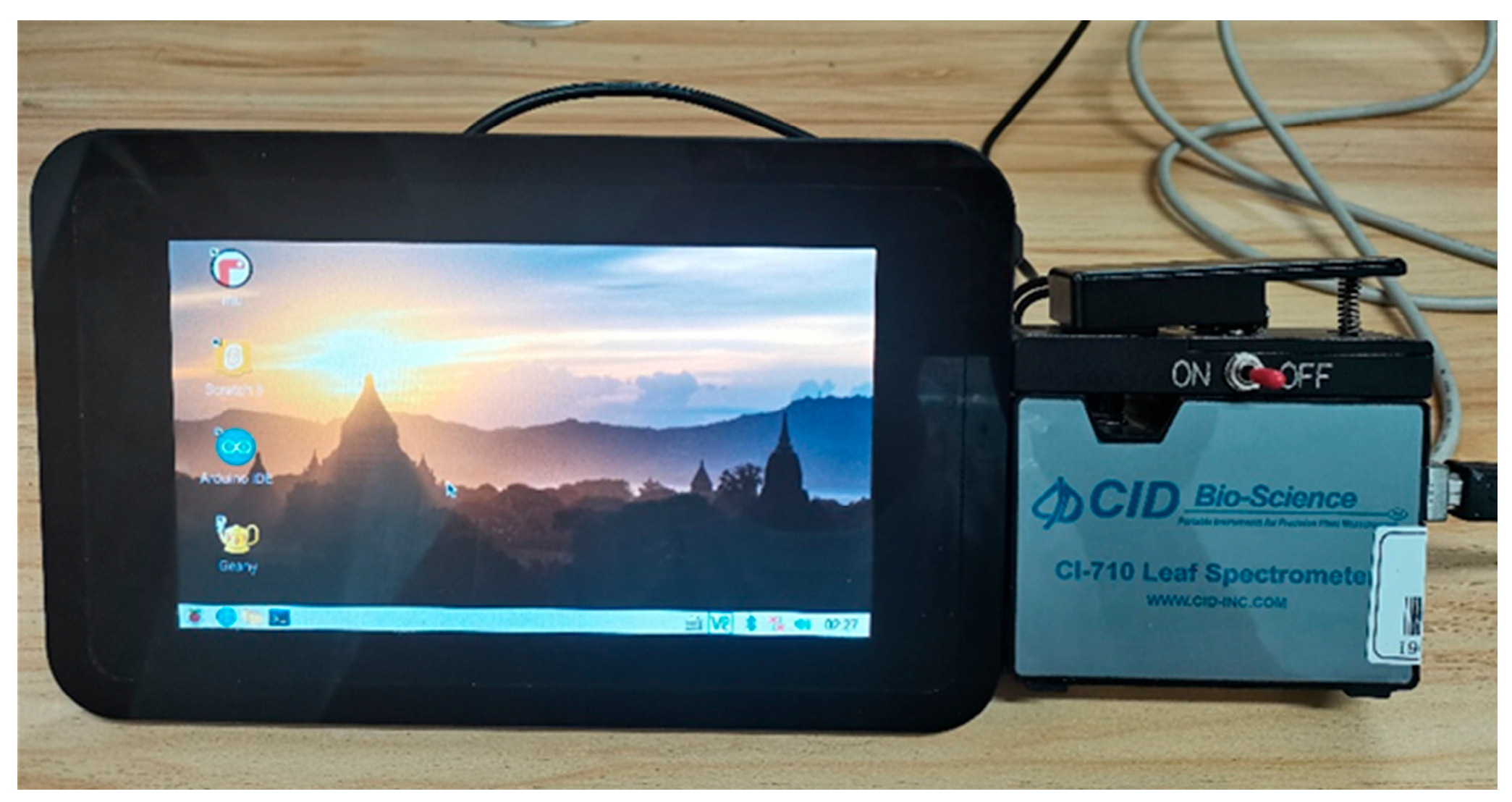
To enable practical application of the optimal chlorophyll and relative water content inversion models, a portable hardware system was developed. The system integrates a CI-710 portable fiber-optic spectrometer (CID Bio-Science, Camas, WA, USA), a Raspberry Pi 4B single-board computer (Raspberry Pi Foundation, Cambridge, UK), and a 7-inch touchscreen display with a resolution of 800 × 480, forming a compact and user-friendly prediction platform (Figure 13).

The pretrained regression model was deployed on a Raspberry Pi using Python (version 3.9), enabling real-time acquisition of near-infrared spectra, automated preprocessing, and immediate parameter prediction. The system features a touchscreen-based graphical user interface, allowing users to collect spectral data and view prediction results directly, significantly enhancing operational convenience and field applicability. Compared to traditional offline methods, this lightweight, low-cost system demonstrated greater practicality and timeliness for rapid drought stress monitoring, confirming its feasibility for deployment in agricultural and ecological settings. To validate system performance and predictive accuracy, 10 maize plants in a greenhouse were selected. For each plant, two leaves were randomly chosen, and five points per leaf were measured using the system. The average of these five predictions was then compared to laboratory measurements of actual chlorophyll content and relative water content to assess the system’s accuracy.

Figure 14 presents a comparison between the system’s predicted values and laboratory-measured values for chlorophyll content and water content. The results showed that the RMSE for chlorophyll was 0.1970 mg/g, and for water content, it was 3.729%. Spectral calibration required less than 10 s, and the entire process—from spectral acquisition to prediction output—was completed within 5 s. These findings confirm that the system enables rapid, non-destructive measurement of chlorophyll and water content in maize leaves, demonstrating high accuracy and practical applicability.

4. Discussion

4.1. The Impact of Drought on Chlorophyll Content and Water Content

The results showed that, under the same growth stage, drought stress led to decreases in both the chlorophyll content and water content in maize leaves. With increasing drought intensity, spectral reflectance significantly increased, especially within the 450–970 nm range, where stressed leaves exhibited higher reflectance than non-stressed ones. Key chlorophyll-sensitive regions, such as the blue (430–470 nm), green peak (500–570 nm), and red-edge (680–740 nm) regions, showed marked reflectance changes due to pigment degradation under drought stress. Although the near-infrared region (700–970 nm) is not a primary chlorophyll absorption zone, it responds to leaf structure and water status, thereby indirectly supporting chlorophyll estimation.

For the water content inversion model, the lower accuracy obtained in this study may be attributed to the limited spectral range. Water-sensitive bands are primarily located in the near-infrared (700–1300 nm) and shortwave infrared (1300–2500 nm) regions, with absorption peaks around 1450 nm, 1940 nm, and 2200 nm. Since only a partial NIR range was used here, model accuracy for water content prediction was constrained.

In conclusion, drought-induced spectral changes provide a feasible basis for quantifying chlorophyll and water content using VIS/NIR reflectance. While the water content model requires further improvement, it still offers valuable insights for drought stress prediction.

4.2. Dimensionality Reduction and Regression Methods

This study demonstrated that dimensionality reduction significantly reduced the number of spectral variables without notably affecting model prediction accuracy, confirming its effectiveness in minimizing spectral data redundancy. After dimensionality reduction, the SPA, Pearson correlation, RF, and SR methods all selected important wavelengths related to chlorophyll and water content. Specifically, the blue region (~460–490 nm) is strongly absorbed by chlorophyll-a and chlorophyll-b [33,34,35], while the NIR region around 894–951 nm corresponds to water absorption features directly related to leaf water status [36]. The Pearson, RF, and SR methods focused on the green peak (~536–560 nm), where maximum reflectance is significantly influenced by leaf internal structure and pigment concentration [33,34], and the red-edge region (~670–750 nm), which is highly sensitive to chlorophyll content and photosynthetic activity, with shifts often linked to vegetation stress [35].

In chlorophyll and water content prediction, the SR and RF models performed best. SR effectively retained chlorophyll-sensitive wavelengths in the green peak and red-edge regions, while RF not only emphasized these bands but also removed irrelevant ones and highlighted NIR water absorption features. Compared to the SPA and Pearson methods, which mainly focus on inter-variable correlations, RF prioritizes direct relationships with the target parameter, thereby better capturing physiologically meaningful spectral information.

In machine learning-based regression modeling, most models predicting chlorophyll content achieved R² values above 0.8, indicating good performance. Considering both prediction accuracy and model complexity, the SR–stacking model performed best, with ${\mathrm{R}}^2$ = 0.8740 and RMSE = 0.2768 mg/g. For water content prediction, the best result was obtained by the RF–stacking model, with ${\mathrm{R}}^2$ = 0.7626 and RMSE = 4.12%. However, this did not meet the target performance threshold, indicating room for improvement.

To further enhance water content inversion accuracy, future work may consider incorporating shortwave infrared (SWIR) bands or applying advanced techniques such as deep learning to optimize model performance based on the existing data.

4.3. Comparison with Previous Studies

Our findings on drought-induced spectral changes in maize are partly consistent with previous reports in both maize and other crops. For instance, Ong et al. [16], in sugarcane, and Ma et al. [14], in mulberry leaves, both identified the blue, green peak, and red-edge regions as sensitive to pigment degradation and water status changes, matching the patterns observed here. In maize, Yang et al. [34] also reported strong chlorophyll sensitivity in these bands across growth stages and canopy layers, supporting the robustness of our spectral region selection under drought stress.

However, our study differs in several important respects. First, unlike Yang et al. [34], who examined chlorophyll variation across developmental stages and vertical leaf positions under general field conditions, we focus on controlled drought gradients to capture stress-specific spectral responses. Second, our modeling framework integrates dimensionality reduction with ensemble regression (SR–stacking and RF–stacking), achieving competitive chlorophyll prediction even within a limited VIS/NIR range (450–970 nm). This contrasts with prior studies [14,16] that relied on extended spectral coverage, including SWIR bands, to enhance water content estimation.

These differences highlight our contribution in demonstrating that meaningful drought-related spectral responses can be extracted from narrower spectral ranges, providing a practical and cost-effective pathway for maize drought monitoring, while also establishing a clear baseline for evaluating the incremental benefits of SWIR integration in future work.

5. Conclusions

In this study, we proposed a non-destructive measurement method based on visible/near-infrared (VIS/NIR) reflectance spectroscopy to estimate chlorophyll and water content in maize leaves under drought stress. By analyzing the spectral reflectance characteristics under different physiological states, we identified key wavelengths associated with chlorophyll and water content, providing a solid data foundation for subsequent model construction.

To improve modeling accuracy and efficiency, we systematically evaluated combinations of dimensionality reduction techniques (e.g., SPA, Pearson correlation, RF, and SR) and regression models (including ensemble methods, such as stacking). The results demonstrated that the SR–stacking model achieved the best performance for chlorophyll prediction, while the RF–stacking model was optimal for water content estimation. These combinations effectively reduced data redundancy and improved predictive accuracy. Overall, the proposed SR–stacking and RF–stacking models offer an efficient, accurate, and non-destructive approach for drought stress monitoring in maize, demonstrating the potential of multi-method integration in spectral modeling.

Furthermore, based on the modeling results, we developed an integrated portable field monitoring system combining spectral acquisition and edge computing capabilities. The system enables real-time and rapid estimation of chlorophyll and water content in maize leaves, preliminarily validating the practical applicability of the proposed method in agricultural settings.

In conclusion, this study not only proposed an efficient spectral prediction framework for multiple physiological traits under maize drought stress but also identified the optimal modeling strategy through systematic evaluation of algorithm combinations. It provides both theoretical support and technical guidance for non-destructive crop monitoring.

Current models lack integration of external factors, such as weather and irrigation, which may constrain their performance in diverse field environments. Future research should consider expanding the input variables and applying more advanced modeling approaches (e.g., deep learning) to enhance model robustness and adaptability, enabling broader applications in smart agriculture.