Abstract
Traditional centralized modeling and fault detection methods for large-scale industrial processes have limitations, including a significant computational load and reduced performance. To address these issues, this paper proposes a distributed dynamic direct orthogonal decomposition method for quality-related fault detection in large-scale industrial processes. This method first decomposes the industrial process to several subunits based on its inherent mechanism. To fully consider the coupling relationship between subunits and improve the communication efficiency among them, the representative variables within each subunit are first selected based on the cosine function. On this basis, regression equations are established between the representative variables of each local subunit and those of its adjacent subunits using LASSO. Then, relevant adjacent unit variables are selected based on the regression coefficients to achieve effective information exchange between the local and adjacent subunits. For the reconstructed local subunits, a dynamic direct orthogonal decomposition method is proposed to achieve quality-related fault detection. In the proposed fault detection method at the subunit level, to better capture the dynamics within the data, the time-delay factor is first introduced to the process variables and the quality variables, and the load matrix of the process variables and the quality variables is obtained using standard partial least squares. Subsequently, the covariance matrix of the load matrix is decomposed based on singular value decomposition to construct an orthogonal decomposition matrix, thereby achieving orthogonal division of the process variables based on the quality variables within each subunit. To derive a more concise detection logic, the Bayesian fusion strategy is adopted to integrate the statistical indicators corresponding to the same type of faults detected in each subunit. Finally, the effectiveness of this method is verified through an industrial example.
1. Introduction
With the growing demand for rapid economic development, modern industrial processes exhibit trends of increasing complexity, expanding scale, and significantly higher levels of automation [1,2]. Consequently, ensuring the safe and stable operation of these processes imposes stringent requirements on the design, monitoring, and management of such systems. As an effective approach to the real-time monitoring of the industrial process status and timely fault identification, fault detection has thus garnered substantial attention from both industry and academia. Existing fault detection methodologies can be categorized into two primary categories based on their underlying principles: model-based methods and data-driven methods [3,4]. Model-based approaches, as the name implies, require detailed mechanistic models of industrial processes. These methods employ techniques such as state estimation, parameter estimation, and parity relations to achieve fault detection. However, given the aforementioned characteristics of contemporary industrial processes, the acquisition of detailed mechanistic models is often impractical or prohibitively costly. Data-driven methods effectively circumvent reliance on mechanistic models by utilizing process data alone and implementing fault detection through machine learning, neural networks, and other related artificial intelligence techniques. Given these advantages, data-driven methods have emerged as the predominant approaches in current process-modeling and fault detection research [5,6].
As noted previously, modern industrial processes typically exhibit large-scale and multi-unit structural characteristics [7]. This inherent complexity poses significant challenges to fault detection methodologies. For such systems, fault detection approaches can be categorized into three primary frameworks based on their architecture: centralized, decentralized, and distributed [8,9]. In the centralized approach, real-time data from all the subunits are transmitted to a central node via a communication network. This node conducts unified fault detection using a global model that incorporates all the subunits and their coupling relationships, ultimately generating system-wide diagnostic results. Although this method ensures global model consistency, it suffers from high computational and communication overhead and tends to encounter performance bottlenecks in large-scale multi-unit industrial systems. The decentralized method equips each subunit with an independent local detector that performs fault detection using only its sensor data [10]. Without information exchange between subunits, the global fault status is determined by the simple aggregation of local results. Consequently, this approach significantly reduces computational and communication costs while simplifying the modeling process. However, it completely disregards coupling relationships between subunits, which is fundamentally inadequate for capturing system-wide faults.
To address these limitations, the distributed framework emerges as an intermediate solution [11]. Subunits share data through localized communication, with each local detector performing fault detection based on its data combined with shared information from neighboring subunits. Global fault detection results are then generated through information fusion techniques. Yin et al. proposed a causality-based multi-perspective subunit partitioning strategy with modified-kernel principal component analysis for early fault detection in large-scale nonlinear industrial processes [12]. Luo et al. investigated data-driven distributed optimal fault detection for interconnected systems with immeasurable neighbor interactions. In this method, algebraic equivalence transformations implicitly incorporate unknown coupling terms into subsystems. This approach preserves fault information propagating through the network topology while enabling optimized residual generator design [13]. Tao et al. developed a distributed adaptive principal component regression algorithm for the online quality monitoring of large-scale industrial dynamic processes [14]. Zhu et al. introduced a multi-block decoupled convolutional neural network to address limitations in extracting features that represent both process states and quality-impacting fault characteristics [15]. Er-Rahmati et al. developed a data-driven mixed-integer linear programming (MILP)-based algorithm for failure detection in large-scale distributed systems: Using piecewise linearization, they formulated an MILP model to derive the optimal failure detector parameters (balancing accuracy and detection time under network/system constraints), proposed a heuristic algorithm for scalability, and validated it via Amazon Cloud, yielding improved detection accuracy and efficiency [16]. Marino et al. developed a machine-learning-based distributed system for industrial IoT fault detection: Using a hybrid Fisher wrapper method for sensor selection and a distributed processing paradigm (to overcome the centralized approach’s drawbacks), it achieved state-of-the-art detection quality and latency in the Tennessee–Eastman (TE) process [17]. However, most existing distributed fault detection methods suffer from two critical limitations: (1) They fail to incorporate effective information-screening mechanisms during inter-unit data exchange, resulting in significant redundancy in communication channels. For instance, in the typical industrial process scenario, existing methods usually transmit most adjacent unit variables without screening, leading to a communication variable redundancy rate of roughly 20–30%. (2) They lack robust mechanisms for detecting quality-related faults.
Quality-related faults refer to disruptions in industrial processes that can severely affect key performance indicators, such as product quality and production yield [18]. These faults constitute a critical category that demands prioritized monitoring in industrial processes. Consequently, quality-related fault detection plays an essential role in modern industrial operations. Such methodologies classify process states into three distinct categories: quality-related faults, quality-unrelated faults, and fault-free operating conditions [19]. Multivariate statistical methods, as a significant branch of data-driven approaches, have become prominent solutions for quality-related fault detection owing to their streamlined model structures and computational efficiencies [20,21,22].
Among multivariate statistical methods, partial least squares (PLS)-based approaches have gained significant prominence in quality-related fault detection [23]. Numerous PLS variants have subsequently emerged: Hu et al. proposed an orthogonal multi-block dynamic PLS method to mitigate false alarms caused by redundant information in quality-relevant subspaces that result from oblique decomposition [24]. Qin et al. developed an analytical PLS framework that addresses solution uncertainty and imperfect optimization objectives through comprehensive correlation analysis between process and quality variables, deriving explicit analytical solutions [25]. For nonlinear extensions of PLS, Si et al. performed generalized singular value decomposition on the covariance of the loading matrices in Kernel PLS (KPLS), achieving orthogonal decomposition of process kernel matrices for effective quality-relevant fault detection [26]. Jiao et al. integrated kernel-sample-equivalent replacement with KPLS to establish a direct linear regression between original variables and quality indicators, enabling accurate fault variable identification [27].
Motivated by the aforementioned challenges, this paper proposes a Distribution Dynamic Direct Orthogonal Decomposition (D3OD) method for quality-related fault detection in plant-wide industrial processes, with a specific focus on benchmark systems, such as the Tennessee–Eastman (TE) process. The core strategy addresses key characteristics of the TE process through the following steps: First, the large-scale system is decomposed to functional subunits using simplified process mechanisms; for instance, this decomposition aligns with the modular structure of the TE process, which comprises feed units, reactor units, separator units, stripper units, and compressor units; second, the cosine similarity function is leveraged to identify representative variables within each local subunit, which reduces redundant data inherent in the unit-level measurements of the TE process; third, LASSO regression is employed to establish mapping relationships between these representative variables and variables from neighboring subunits, in which regression coefficients screen for relevant neighboring variables; for the reconfigured subunits that integrate screened local and neighboring information, a dynamic direct orthogonal decomposition approach is adopted to enable local quality-related fault detection, which is tailored to capture the time-varying dynamic characteristics of the TE process; finally, a Bayesian fusion strategy is introduced to integrate fault-specific statistical indicators across all the subunits, streamlining the global detection logic that is often cumbersome in the multi-unit monitoring of the TE process, to enhance detection efficiency. The primary contributions are summarized as follows:
- (1)
- A D3OD method is proposed for quality-related fault detection of plant-form industrial processes;
- (2)
- A distributed subunit reconstruction strategy, incorporating cosine similarity functions and LASSO regression, is proposed. This strategy maintains essential information exchange between local and neighboring subunits while effectively eliminating communication redundancy, thus, significantly improving communication transmission efficiency;
- (3)
- For reconfigured local subunits, a dynamic direct orthogonal decomposition approach is developed. This approach achieves orthogonal decomposition of the process variable space based on quality indicators. This enables the detection of the process status and fault types via process variables—even when quality indicators cannot be measured in real time.
The remainder of this paper is structured as follows: Section 2 presents the proposed distributed subunit reconstruction strategy, incorporating cosine similarity and LASSO regression. Section 3 details the D3OD methodology and the comprehensive quality-oriented monitoring framework, consisting of three components: Section 3.1 introduces the dynamic direct orthogonal decomposition approach for reconfigured local subunits. Section 3.2 introduces the establishment of the detection statistics and the online monitoring process. Section 3.3 describes the Bayesian fusion-based global detection indicator and the overall fault detection process of the proposed method. Section 4 validates the proposed methodology through an industrial case study. Section 5 concludes the paper and presents future research directions.
2. Establishment of Distributed Subunits
Consider a plant-wide industrial process that contains process variables and quality variables. During the offline modeling, collect n samples of the process and quality variables under normal conditions, which can be expressed as
Based on the simplified internal mechanisms of the industrial process, which do not require detailed mechanistic models, the process is assumed to be decomposable to subunits. Thus, the process variables can be divided as
where denotes the process variable matrix of the th subunit, with n representing sample size and the variable dimension. This matrix can be expressed as
Building upon the previously established decomposed subunit structure, a novel distributed subunit approach for fault detection is proposed. For distributed fault detection, addressing coupling relationships between local and neighboring subunits is critical. However, incorporating all the neighboring information would induce substantial redundancy, imposing excessive communication and computational burdens. Since the cosine similarity function is effective for identifying representative variables within local subunits [28], it is utilized herein for variable selection. Specifically, the cosine similarity between variables and in the subunit is computed as
When the cosine similarity () exceeds a predefined threshold (), the process variables ( and ) are deemed as informationally redundant. Here, is a predefined threshold, typically determined based on academic conventions or empirical validation. A review of the literature shows that is a suitable value [29], and, thus, this value is also adopted in this study.
Based on this criterion, representative variables for local subunits are selected according to the following rule:
- (1)
- Randomly select one process variable () from the local subunit variable matrix () and add it to the representative variable set ();
- (2)
- Perform the following operations on each remaining variable (): Compute the cosine similarities with all the variables in . If the calculated is greater than the threshold (), the variable () should be discarded; else, add to ;
- (3)
- Iterate step (2) until all the variables are processed.
This procedure yields the representative variable matrix () for the local subunit. Next, neighboring subunit variables of the local subunit are aggregated into matrix . As a special case of elastic net regression, LASSO enables simultaneous variable selection and coefficient estimation through -norm penalization [30]. This capability allows selecting relevant neighboring variables while addressing collinearity among neighboring unit variables. Consequently, LASSO regression is used to establish the relationship between the representative matrix () and the neighbor variable matrix (), and this relationship can be expressed as
where controls the sparsity regularization intensity. Variables in that correspond to constitute the communication variable space (). This space is then combined with the local subunit variable matrix () to form the reorganized subunit (), which incorporates information interactions with selected neighboring variables. For the unknown parameter (), we use the 10-fold cross-validation method provided by the LASSO functions in the MATLAB 2022a Toolbox to determine its optimal value.
Each subunit matrix () undergoes the identical information-interaction-based reconstruction process to complete the primary phase of distributed detection, i.e., information-interaction-based subunit reconstruction. Subsequently, the dynamic direct orthogonal decomposition method for the reconstructed subunits is introduced.
3. Dynamic Direct Orthogonal-Decomposition-Based Quality-Related Fault Detection
3.1. Dynamic Direct Orthogonal Decomposition Method
For the reconstructed local subunit () and quality variable matrix (), time-lag matrices ( and ) are constructed to capture dynamic features, which can be expressed as
where h is the time-lag factor. This factor is determined specifically for the PLS model through cross-validation. For the augmented dynamic matrices ( and ) derived through time-lag embedding, a PLS model is established through the following procedure [31]:
- Standardize the process variable matrix () and quality variable matrix () to zero mean and unit variance. Initialize , and set ;
- Initialize the latent vector () with an arbitrary column from the standardized quality matrix ();
- Calculate the weight vector () through ;
- Calculate the score vector, weight coefficient, and update () as
- Loop through steps 2 to 4 until the score vector () converges, and then proceed with the subsequent operations;
- Calculate the process variable load vector ();
- Update the residual matrix ();
- Let , return to step 2, and continue until i reaches the predetermined value (a), completing the extraction of all the latent variables.
For the number (a) of latent variables, the cross-validation method is used as the essential tool. The relationship between the augmented process matrix () and quality matrix () is established through the PLS decomposition, which can be expressed as
where and represent the score matrices of the process and quality variables, and are the loading matrices of the process and quality variables, and and are the residual matrices.
As introduced above, the traditional PLS method cannot effectively achieve orthogonal decomposition of the process space, which causes information leakage and leads to missed detections and false positives. For example, in the TE process, for quality-unrelated faults, the fault detection rate of the quality-related subspace obtained through PLS exceeds ; that is, the quality-unrelated faults are wrongly diagnosed as quality-related faults. To address this issue, building on the aforementioned PLS modeling and the obtained load matrices ( and ), we propose a strategy of direct orthogonal decomposition. Since time-lag factors were introduced to process and quality variables during the initial processing to account for the dynamic characteristics of the process, we named the improved method the Dynamic Direct Orthogonal Decomposition Strategy.
For the load matrices ( and ) of the obtained process variables and quality variables, establish the covariance matrix () between them, which can be expressed as
For the covariance matrix () obtained above, performing SVD processing on it can yield the following form:
where , , is a diagonal matrix composed of eigenvalues. Based on the obtained matrices ( and ), establish two projection matrices as
Based on the established projection matrices, project the process matrix in these two subspaces:
where and represent the quality-related and quality-unrelated subspaces within the process matrices, respectively.
Through the above process, we constructed two projection matrices by performing SVD on the covariances of process and quality variables. Process variables are mapped to these two subspaces and decomposed to two mutually orthogonal parts. Using this decomposition, we introduce below how to establish corresponding detection indicators in these two subspaces.
Remark 1.
Considering that the covariance matrix () has dimensions of , where denotes the dimension of the quality variables, denotes the dimension of the process variables in the reconstructed subunit, and h denotes the introduced time-lag factor, in typical industrial processes, the condition is satisfied, and, thus, . Therefore, the covariance matrix () is a row-full-rank matrix. Consequently, performing SVD on it yields a singular value matrix of the form shown in Equation (11), consisting of a full-rank singular value matrix () and a zero matrix (), where has dimensions . Based on the above analysis, the right singular value matrix () is naturally decomposed to two matrices ( and ) according to the form of the singular value matrix. Hence, the decomposition of the covariance matrix () yields the result presented in Equation (11).
3.2. Detection Statistics and Online Monitoring
During the online detection process, when the new process variable data () arrive, they are first standardized using the mean and standard deviation from offline training data. Then, based on the aforementioned strategy for reconstructing local subunits, relevant interaction information from neighboring units is screened out. The reconstruction of the local subunit is then completed to obtain . Subsequently, the time-lag factor (h) is introduced to form the augmented matrix ().
For the reconstructed local subunit (), the aforementioned projection matrices ( and ) are used to decompose it to two mutually orthogonal components, which can be expressed as
For the two formed parts, and Q statistics are used as the essential monitoring indicators [32]. For the established quality-related part (), the statistic is used as the detection statistic, which can be calculated as
where the matrix can be calculated during the offline modeling process, which can be calculated as
For the obtained statistic, the corresponding threshold is calculated through the distribution:
where . For the established quality-unrelated part (), the Q statistic is used as the detection statistic to test it, which is calculated as
The corresponding threshold can be calculated through the distribution. Here are the specific steps:
where and denote the mean value and the variance of the diagonal elements of , respectively, and . The corresponding local detection logic is shown as follows:
- (1)
- && Fault free;
- (2)
- Quality-related fault;
- (3)
- Quality-unrelated fault.
3.3. Bayesian Fusion and Monitoring Logic
Using the above process, we established two statistical indicators, and , for each reconstructed local subunit to detect the faults contained in the quality-related subspace and the quality-unrelated subspace. Both belong to the local fault detection for each subunit. However, for a large-scale industrial process, we hope not only to complete local fault detection for each subunit but also to achieve global fault detection. Moreover, fewer monitoring metrics result in simpler detection logic. Consequently, the Bayesian fusion method is used to combine these two local monitoring statistics for the local subunit [10]. Detailed calculation steps are presented as follows:
In addition, , , , and can be computed in the same way, and and . Then, the combined monitoring statistics ( and ) can be calculated as
The corresponding threshold of the and monitoring statistics is . To sum up, for the global unit, there are two monitoring statistics to monitor it, where monitors the quality-related part, and monitors the quality-unrelated part. The corresponding global detection logic is shown as follows:
- (1)
- Fault free;
- (2)
- Quality-related fault;
- (3)
- Quality-unrelated fault.
| Algorithm 1 D3OD-based quality-related fault detection |
|
|
3.4. Complexity Analysis
The analysis of the offline computational load for Algorithm 1 is divided into key steps as follows:
- (1)
- Offline Step 1: This step mainly involves screening representative variables within each subunit using the cosine similarity function. For each of the local subunits, if a single subunit contains process variables, the computational complexity of calculating the cosine similarity between all the pairs of variables within the subunit is . For subunits in total, the overall complexity of this step is ;
- (2)
- Offline Step 2: To establish the mapping relationship between the representative variables of each local subunit and the variables of adjacent subunits, LASSO regression is used for variable selection and regression modeling. For a single subunit, the complexity of the LASSO regression depends on the number of offline training samples (n) and the number of adjacent subunit variables (); the complexity for one subunit is . Extending to subunits, the total complexity of this step is ;
- (3)
- Offline Step 3: This step is the core of the offline training phase, consisting of two key operations: PLS decomposition and SVD processing of the covariance matrix, both of which contribute significantly to the offline computational load.
For each reconstructed local subunit, a time-lag matrix is first constructed (with a time-lag step of h) to capture process dynamics and then a latent variables are extracted through the iterative calculation of load vectors and score vectors. For one subunit, the complexity is (scaling with the sample size (n), time-lag step (h), number of subunit variables (), and number of latent variables (a)). For subunits, the total complexity is .
Based on the load matrices of the process and quality variables obtained from PLS, the covariance matrix () is constructed, and SVD is performed to obtain projection matrices for quality-related and quality-unrelated subspaces. For one subunit, the complexity of the SVD depends on the numbers of quality variables (), subunit variables (), and time-lag step (h) and is . For subunits, the total complexity is .
Together, these two operations form the main body of the offline computational load, especially PLS decomposition, which involves iterative matrix operations and is highly dependent on the sample size and latent variable count;
- (4)
- Offline Step 4 (Threshold Calculation): Thresholds for and Q statistics are calculated based on the F-distribution and chi-squared distribution, respectively. This step only involves fixed-form statistical formula calculations, with a computational complexity of .
Summing the complexities of the above offline steps, the total offline computational load is dominated by the dynamic direct orthogonal decomposition, followed by the LASSO regression and representative variable selection, while the threshold calculation has almost no impact. The total offline complexity can be expressed as follows: .
Among these terms, contributes the most to the overall offline computational load, which is the key factor determining the offline training efficiency of the algorithm.
4. Case Studies
To intuitively demonstrate the performance of the proposed method, two widely used metrics: the false alarm rate (FAR) and fault detection rate (FDR), are adopted as evaluation criteria. Between them, FAR refers to the probability that the statistic exceeds the preset threshold when there is no fault in the process, while FDR refers to the probability that the statistic exceeds the preset threshold when a fault occurs in the process. Obviously, for a fault detection method, the higher the FDR and the lower the FAR, the better its detection performance. For quality-oriented fault detection, faults need to be labeled and distinguished (quality-related/quality-unrelated faults). Specifically, when a quality-related fault occurs, the higher the FDR of the quality-related subspace, the better the performance of the method; when a quality-unrelated fault occurs, the quality-related subspace should avoid detecting this fault (i.e., a lower FDR), while the quality-unrelated subspace should maintain a high FDR. In summary, the effectiveness criteria for a high-performance quality-oriented fault detection method are as follows: For quality-related faults, the quality-related subspace should have a high FDR; for quality-unrelated faults, the quality-related subspace should have a low FAR.
This experiment is based on the TE process, a standard testing platform in the field of industrial process monitoring proposed by Downs and Vogel [33]. This process simulates the complete process chain of polyethylene synthesis by the gas-phase method, including five core units: the reactor, condenser, separator, stripper, and compressor, with the characteristics of multivariable coupling and 21 default failure modes. It provides an ideal scenario for the experimental verification of most monitoring algorithms. The TE process contains a total of 52 variables, including 22 XMEASs for measurement variables, 11 XMVs for operation variables, and 19 state variables. The TE process also contains four gases, represented by A, C, D, and E, two liquid products (G and H), byproducts (F), and an inert gas (B); the relevant irreversible exothermic chemical reactions in the TE process can be expressed as
where G is the main product, and F is the byproduct. Based on this process, this experiment uses the improved PLS algorithm to model and analyze the quality-related faults and quality-unrelated faults in the process to detect the faults. In this paper, 22 measurement variables and 11 operation variables are selected to construct the process variable space (), and the measurement variables, XMEASs (35), are selected to form the quality-related variables (). The results of the fault classification in the TE process in the literature are used as the standard.
In this part, component G from Process 9 is adopted as the quality variable. According to the internal mechanism of the TE process, it can be decomposed to five subunits: Unit 1 (feed), Unit 2 (reactor), Unit 3 (separator), Unit 4 (stripping tower), and Unit 5 (compressor). The variables contained within each operation unit are also shown in Table 1. The original five units were preprocessed using the proposed method, presented in Section 2, and the adjacent units were screened. After screening, the screened variables were reconstructed with the variables of the original units to obtain five new subunits.

Table 1.
Variables contained within each operation unit of the TE process ((a) represents the measured variables and (b) represents the manipulated variables).
To verify the effectiveness of the method proposed in this paper, in the experimental simulation section, we made a detailed comparison of three faults of two types. In addition, PLS, OPLS, MOPLS, TPCR, and TPLS methods were used as comparison objects. For the experiment, we used 500 offline normal samples and 960 online samples as the dataset. The online samples are divided into 160 normal samples and 800 fault samples. With this dataset, the total runtime of the proposed method is approximately 8 s.
4.1. Quality-Related Faults
For quality-related fault IDV(2), the D3OD, PLS, OPLS, TPCR, TPLS, and MOPLS methods are tested. Fault IDV(2) is a step change in the reactor’s outlet temperature. This fault is manifested as a sudden step deviation in the reactor’s outlet temperature (T-related parameters in process variables) from the normal operating conditions. It is a temperature-related disturbance fault and will directly affect the reaction efficiency and product characteristics. Under this fault, the quality variable variation curve is shown in Figure 1a. It is obvious that from the occurrence of the fault until its end, it has hurt the quality variable. Under this fault, the FDRs of the PLS, OPLS, TPCR, TPLS, MOPLS, and D3OD methods are shown in Table 2, and the corresponding detection performances of the different methods are shown in Figure 1. Furthermore, for the proposed D3OD method, the subunit-level detection results are presented in Figure 2.
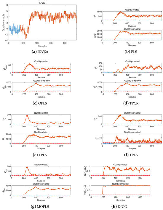
Figure 1.
Detection performances of the different methods for fault IDV(2).
Table 2.
FDRs of the PLS, OPLS, TPCR, TPLS, MOPLS, and D3OD methods in the quality-related subspace for quality-related faults IDV(2) and IDV(6).
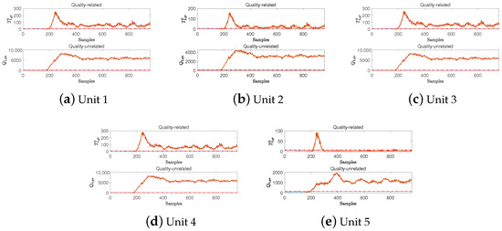
Figure 2.
Detection performances of the D3OD method for fault IDV(2) in different units.
For quality-related fault IDV(6), the D3OD, PLS, OPLS, TPCR, TPLS, and MOPLS methods proposed are tested. Fault IDV(6) refers to a sudden step change in the inlet temperature of the reactor coolant at the 160th sampling moment, and it persists, disrupting the thermal balance of the reactor, interfering with the reaction rate and product characteristics, and subsequently affecting the operation of downstream units in a chain reaction. The corresponding quality variables are shown in Figure 3a. It is obvious that from the occurrence of the fault until its end, it has had an adverse impact on the quality variable. Under this fault, the FDRs of the OPLS, TPCR, and D3OD methods are shown in Table 2, and the corresponding detection performances of the different methods are shown in Figure 3. Furthermore, for the proposed D3OD method, the subunit-level detection results are presented in Figure 4.
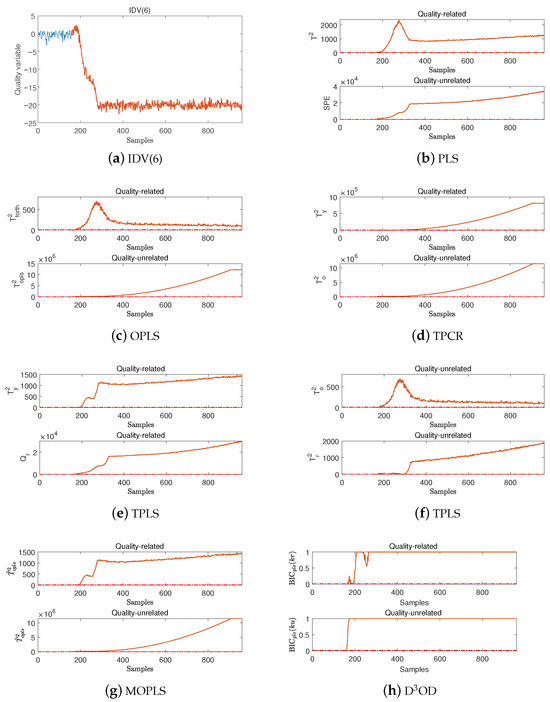
Figure 3.
Detection performances of the different methods for fault IDV(6).
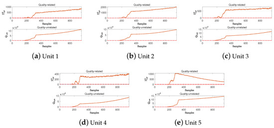
Figure 4.
Detection performances of the D3OD method for fault IDV(6) in different units.
By observing the above simulation results, it can be found that the FDRs of the PLS, OPLS, TPCR, TPLS, MOPLS, and D3OD methods in their quality-related subspace are all very high, all exceeding . Therefore, by combining the corresponding detection logic of each method, it can be found that all three methods can accurately determine the types of the above two faults as quality-related faults, which verifies the effectiveness of the method proposed in this paper. Further, by observing Table 2, it can be found that for fault IDV(2), the FDR of the proposed D3OD method is , which is higher than those of the TPCR and MOPLS methods. In addition, the proposed D3OD method has a higher FDR than the OPLS and MOPLS methods for IDV(6). This also means that compared with these methods, the method proposed in this paper has a higher detection rate for quality-related faults.
4.2. Quality-Unrelated Faults
For quality-unrelated fault IDV(4), the D3OD, PLS, OPLS, TPCR, TPLS, and MOPLS methods are tested. Fault IDV(4) is a step change in the feed temperature of the reactor, which usually occurs suddenly at the 160th sampling moment and maintains a deviation continuously. This fault interferes with the initial reaction conditions of the reactor, alters the reaction rate and product composition, and thereby triggers a chain reaction that impacts the operational stability of downstream units (e.g., separation units). Under this fault, the variation curve of the quality variables is shown in Figure 5a. It is evident that from the fault onset to termination, the fault exerts a significant adverse impact on the quality variables. The FDRs of the OPLS, TPCR, and D3OD methods under this fault are presented in Table 3 and Table 4, and the detection performances of the different methods are illustrated in Figure 5. Furthermore, the local subunit detection results of the proposed D3OD method are shown in Figure 6.
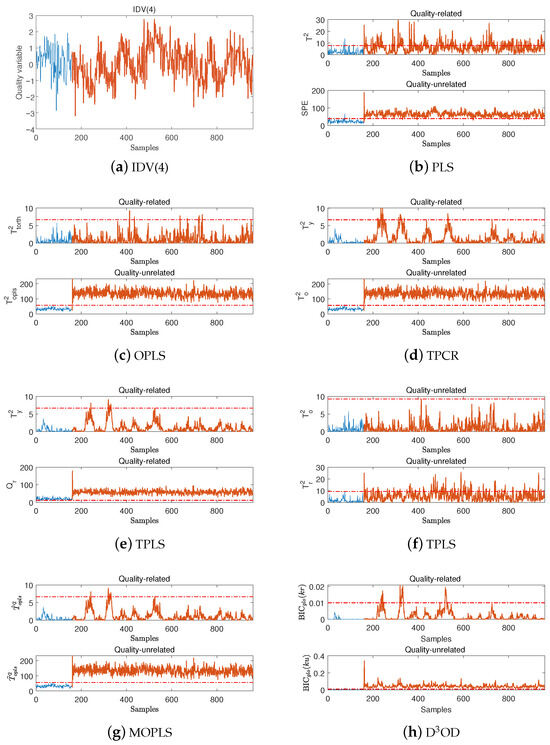
Figure 5.
Detection performances of the different methods for fault IDV(4).
Table 3.
FARs of the PLS, OPLS, TPCR TPLS, MOPLS, and D3OD methods in the quality-related subspace for quality-unrelated faults IDV(4) and IDV(14).
Table 4.
FDRs of the PLS, OPLS, TPCR TPLS, MOPLS, and D3OD methods in the quality-related subspace for quality-unrelated faults IDV(4) and IDV(14).
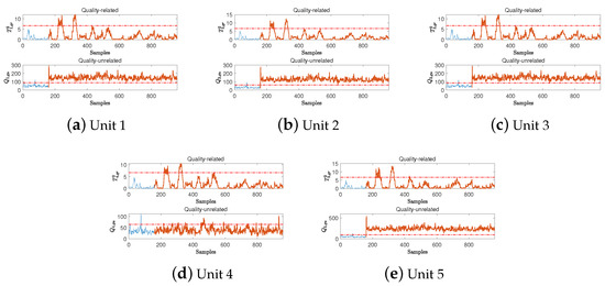
Figure 6.
Detection performances of the D3OD method for fault IDV(4) in different units.
For quality-unrelated fault IDV(14), the proposed D3OD method was tested alongside PLS, OPLS, TPCR, TPLS, and MOPLS. Fault IDV(14) is a viscosity fault of the reactor’s coolant valve, which prevents normal regulation of the coolant flow rate. This fault disrupts the thermal balance of the reactor, causes abnormal temperature fluctuations, and impairs the operational stability of downstream units. It is a typical actuator-jamming disturbance; the corresponding quality variables are shown in Figure 7a. Notably, the fault induces a persistent adverse impact on quality variables throughout its duration. Under this fault, the FDRs of the OPLS, TPCR, and D3OD methods are listed in Table 3 and Table 4, and the detection performance of each method is depicted in Figure 7. Additionally, the local subunit detection results of D3OD are presented in Figure 8.
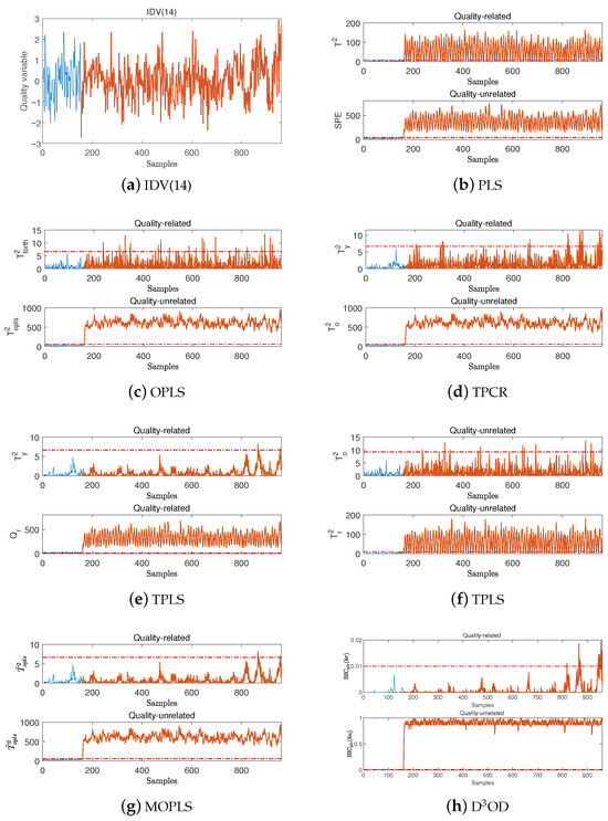
Figure 7.
Detection performances of the different methods for fault IDV(14).
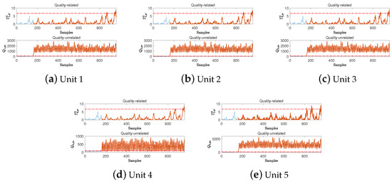
Figure 8.
Detection performances of the D3OD method for fault IDV(14) in different units.
From the above test results, it can be observed that for quality-unrelated faults IDV(4) and IDV(14), within the quality-related subspaces of the different methods, the TPLS method exhibits the highest FAR, reaching and incorrectly diagnoses these two faults as quality-related ones, while although the PLS method has a relatively lower FAR, it still shows a high FAR of for fault IDV(14). This aligns with the description of the limitations of PLS in the previous section; that is, PLS fails to achieve orthogonal decomposition of the process variable space based on quality indicators. In contrast, the OPLS, TPCR, MOPLS, and D3OD methods all demonstrate low FARs (all were below ), and for fault IDV(14), the detection performances of MOPLS and D3OD are better than those of the other methods.
Furthermore, in the quality-unrelated subspaces of these methods, most achieve high FDRs. Among these methods, OPLS and D3OD even reach an FDR of for both IDV(4) and IDV(14). In summary, these results further verify the effectiveness of the proposed D3OD method.
5. Conclusions
This paper addresses the key challenges of high computational burden and performance limitations inherent in traditional centralized modeling and fault detection methods for large-scale industrial processes. To overcome these limitations, a new D3OD method is proposed, specifically for quality-related fault detection. The core approach involves strategically decomposing complex industrial processes to manageable subsystems based on intrinsic process mechanisms. Recognizing the crucial roles of subsystem interactions, the cosine function and LASSO regression effectively and explicitly model the coupling relationship between each local subunit and its adjacent subunits. In this way, the most relevant adjacent unit variables can be selected, significantly improving the efficiency of information exchange, which is crucial in distributed monitoring. For each reconfigured local subunit, the dynamic direct orthogonal decomposition method is applied to achieve effective quality-related fault detection at the subunit level. To further simplify the detection process and derive a more concise detection logic, the Bayesian fusion strategy was introduced. This strategy intelligently integrates the statistical indicators corresponding to the same fault type detected across different subunits. The effectiveness of the proposed D3OD framework was verified through the TE process. In quality-related fault detections (IDV(2) and IDV(6)), the global statistic of D3OD achieved FDRs of and , outperforming those of the MOPLS method ( and ) in key cases. Its dynamic direct orthogonal decomposition, with time-lag embedding and strict subspace orthogonality, avoided the information leakage of traditional PLS (e.g., PLS misclassifies of quality-unrelated faults as quality-related in IDV(4)). For quality-unrelated faults, D3OD had low FARs in the quality-related subspace ( for IDV(4) and for IDV(14))—far lower than those of PLS ( and )—and FDRs in the quality-unrelated subspace.
At present, the D3OD algorithm, based on linear PLS and orthogonal decomposition, has limited adaptability to strong nonlinear processes. In the future, we will integrate the kernel methods and extend the algorithm to the nonlinear domain, thereby solving the coupling modeling problem of nonlinear subsystems. In addition, the Bayesian fusion method adopted in this study has limitations, primarily stemming from the conditional independence assumption for monitoring statistics of local subunits in fault or normal states. This simplification may cause deviations in fusion accuracy. To address this in future work, we plan to explore advanced probabilistic models that better characterize the dependency structure between monitoring statistics while retaining interpretability. These extensions will enable more accurate global fault detection in complex, strongly coupled industrial processes.
Author Contributions
Conceptualization, J.Y.; methodology, J.Y. and Y.W.; software, Y.W.; validation, J.Y., Y.W. and H.M.; formal analysis, H.M.; writing—original draft preparation, J.Y.; writing—review and editing, Y.W.; supervision, H.M. All authors have read and agreed to the published version of the manuscript.
Funding
This work was supported by the Wuxi Science and Technology Development Fund Project (under grants K20241048 and K20241029), the Wuxi University Research Start-up Fund for Introduced Talents (under grant 2023r020), and Fundamental Research Funds for the Central Universities (under grant JUSRP202501036.
Data Availability Statement
The original contributions presented in this study are included in the article. Further inquiries can be directed to the corresponding author.
Conflicts of Interest
The authors declare no conflicts of interest.
References
- Ma, X.; Chen, T.; Wang, Y. Dynamic process monitoring based on dot product feature analysis for thermal power plants. IEEE/CAA J. Autom. Sin. 2025, 12, 563–574. [Google Scholar] [CrossRef]
- Jiang, Q.; Jiang, J.; Zhong, W.; Yan, X. Optimized gaussian-process-based probabilistic latent variable modeling framework for distributed nonlinear process monitoring. IEEE Trans. Syst. Man Cybern. Syst. 2022, 53, 3187–3198. [Google Scholar] [CrossRef]
- Ding, S.X. Data-driven design of monitoring and diagnosis systems for dynamic processes: A review of subspace technique based schemes and some recent results. J. Process Control 2014, 24, 431–449. [Google Scholar] [CrossRef]
- Ding, S.X.; Yang, Y.; Zhang, Y.; Li, L. Data-driven realizations of kernel and image representations and their application to fault detection and control system design. Automatica 2014, 50, 2615–2623. [Google Scholar] [CrossRef]
- Gao, L.; Li, D.; Chen, Z.; Ding, S.X.; Luo, H. Sir-aided dynamic canonical correlation analysis for fault detection and isolation of industrial automation systems. IEEE Trans. Ind. Electron. 2023, 71, 11560–11570. [Google Scholar] [CrossRef]
- Wang, Y.; Zhou, D.; Chen, M. Dynamic related component analysis for quality-related process monitoring with applications to thermal power plants. Control Eng. Pract. 2023, 132, 105426. [Google Scholar] [CrossRef]
- Jiang, Q.; Chen, S.; Yan, X.; Kano, M.; Huang, B. Data-driven communication efficient distributed monitoring for multiunit industrial plant-wide processes. IEEE Trans. Autom. Sci. Eng. 2021, 19, 1913–1923. [Google Scholar] [CrossRef]
- Yao, L.; Ge, Z. Industrial big data modeling and monitoring framework for plant-wide processes. IEEE Trans. Ind. Inform. 2020, 17, 6399–6408. [Google Scholar] [CrossRef]
- Peng, X.; Ding, S.X.; Du, W.; Zhong, W.; Qian, F. Distributed process monitoring based on canonical correlation analysis with partly-connected topology. Control Eng. Pract. 2020, 101, 104500. [Google Scholar] [CrossRef]
- Ma, L.; Dong, J.; Hu, C.; Peng, K. A novel decentralized detection framework for quality-related faults in manufacturing industrial processes. Neurocomputing 2021, 428, 30–41. [Google Scholar] [CrossRef]
- Ge, Z.; Chen, J. Plant-wide industrial process monitoring: A distributed modeling framework. IEEE Trans. Ind. Inform. 2015, 12, 310–321. [Google Scholar] [CrossRef]
- Yin, M.; Wang, W.; Tian, J.; Jiang, J. Distributed incipient fault detection with causality-based multi-perspective subblock partitioning for large-scale nonlinear processes. Process Saf. Environ. Prot. 2024, 185, 492–510. [Google Scholar] [CrossRef]
- Li, B.; Yang, Y. Data-driven optimal distributed fault detection based on subspace identification for large-scale interconnected systems. IEEE Trans. Ind. Inform. 2023, 20, 2497–2507. [Google Scholar] [CrossRef]
- Tao, Y.; Shi, H.; Song, B.; Tan, S. A distributed adaptive monitoring method for performance indicator in large-scale dynamic process. IEEE Trans. Ind. Inform. 2023, 19, 10425–10433. [Google Scholar] [CrossRef]
- Zhu, J.; Shi, H.; Song, B.; Tao, Y.; Tan, S. Convolutional neural network based feature learning for large-scale quality-related process monitoring. IEEE Trans. Ind. Inform. 2021, 18, 4555–4565. [Google Scholar] [CrossRef]
- Er-Rahmadi, B.; Ma, T. Data-driven mixed-Integer linear programming-based optimisation for efficient failure detection in large-scale distributed systems. Eur. J. Oper. Res. 2022, 303, 337–353. [Google Scholar] [CrossRef]
- Marino, R.; Wisultschew, C.; Otero, A.; Lanza-Gutierrez, J.M.; Portilla, J.; Torre, E.D. A machine-learning-based distributed system for fault diagnosis with scalable detection quality in industrial IoT. IEEE Internet Things J. 2020, 8, 4339–4352. [Google Scholar] [CrossRef]
- Zhou, L.; Wang, Y.; Wu, Y.; He, S.; Song, Z. Quality-relevant modeling and monitoring of industrial cyber-physical systems: The semi-supervised dynamic latent variable models. IEEE Trans. Ind. Cyber-Phys. Syst. 2024, 3, 39–47. [Google Scholar] [CrossRef]
- Zhang, X.; Ma, L.; Peng, K.; Zhang, C.; Shahid, M.A. A cloud–edge collaboration based quality-related hierarchical fault detection framework for large-scale manufacturing processes. Expert Syst. Appl. 2024, 256, 124909. [Google Scholar] [CrossRef]
- Sun, R.; Wang, Y. Key-performance-indicator-related fault detection based on deep orthonormal subspace analysis. IEEE Trans. Ind. Inform. 2024, 20, 7249–7258. [Google Scholar] [CrossRef]
- Liu, Q.; Yang, C.; J, S. Qin, Semi-supervised dynamic latent variable regression for prediction and quality-relevant fault monitoring. IEEE Trans. Control Syst. Technol. 2024, 32, 1156–1168. [Google Scholar] [CrossRef]
- Yang, J.; Wang, J.; Ye, Q.; Xiong, Z.; Zhang, F.; Liu, H. A novel fault detection framework integrated with variable importance analysis for quality-related nonlinear process monitoring. Control Eng. Pract. 2023, 141, 105733. [Google Scholar] [CrossRef]
- Lin, X.; Sun, R.; Wang, Y. Improved key performance indicator-partial least squares method for nonlinear process fault detection based on just-in-time learning. J. Frankl. Inst. 2023, 360, 1–17. [Google Scholar] [CrossRef]
- Hu, C.; Luo, J.; Kong, X.; Xu, Z. Orthogonal multi-block dynamic PLS for quality-related process monitoring. IEEE Trans. Autom. Sci. Eng. 2024, 21, 3421–3434. [Google Scholar] [CrossRef]
- Qin, Y.; Lou, Z.; Wang, Y.; Lu, S.; Sun, P. An analytical partial least squares method for process monitoring. Control Eng. Pract. 2022, 124, 105182. [Google Scholar] [CrossRef]
- Si, Y.; Wang, Y.; Zhou, D. Key-performance-indicator-related process monitoring based on improved kernel partial least squares. IEEE Trans. Ind. Electron. 2020, 68, 2626–2636. [Google Scholar] [CrossRef]
- Jiao, J.; Zhen, W.; Wang, G.; Wang, Y. KPLS-KSER based approach for quality-related monitoring of nonlinear process. ISA Trans. 2021, 108, 144–153. [Google Scholar] [CrossRef] [PubMed]
- Xia, P.; Zhang, L.; Li, F. Learning similarity with cosine similarity ensemble. Inf. Sci. 2015, 307, 39–52. [Google Scholar] [CrossRef]
- Zhang, J.; Chen, M.; Hong, X. Monitoring multimode nonlinear dynamic processes: An efficient sparse dynamic approach with continual learning ability. IEEE Trans. Ind. Inform. 2022, 19, 8029–8038. [Google Scholar] [CrossRef]
- Ranstam, J.; Cook, J.A. LASSO regression. J. Br. Surg. 2018, 105, 1348. [Google Scholar] [CrossRef]
- Jong, S.D. SIMPLS: An alternative approach squares regression to partial least. Chemom. Intell. Lab. Syst. 1993, 18, 2–263. [Google Scholar] [CrossRef]
- Ma, H.; Wang, Y.; Liu, X.; Yuan, J.; Zhou, Y. Sliding window-aided recursive efficient kernel decomposition for KPI-oriented fault detection of complex industrial processes. Knowl. Based Syst. 2025, 314, 113140. [Google Scholar] [CrossRef]
- Downs, J.J.; Vogel, E.F. A plant-wide industrial process control problem. Comput. Chem. Eng. 1993, 17, 245–255. [Google Scholar] [CrossRef]


Disclaimer/Publisher’s Note: The statements, opinions and data contained in all publications are solely those of the individual author(s) and contributor(s) and not of MDPI and/or the editor(s). MDPI and/or the editor(s) disclaim responsibility for any injury to people or property resulting from any ideas, methods, instructions or products referred to in the content. |
© 2025 by the authors. Licensee MDPI, Basel, Switzerland. This article is an open access article distributed under the terms and conditions of the Creative Commons Attribution (CC BY) license (https://creativecommons.org/licenses/by/4.0/).