Productivity Prediction Model of Tight Oil Reservoir Based on Particle Swarm Optimization–Back Propagation Neural Network

Abstract

Single-well productivity is a crucial metric for assessing the effectiveness of petroleum reservoir development. The accurate prediction of productivity is essential for achieving the efficient and economical development of oil–gas reservoirs. Traditional productivity prediction methods (empirical formulae and numerical simulation) are limited to specific reservoir types. There are few influencing factors, and a large number of ideal assumptions are made for the assumed conditions when predicting productivity. The application scenario is ideal. However, in tight oil reservoirs, numerous factors affect productivity, and their interactions exhibit significant complexity. Continuing to use traditional reservoir productivity prediction methods may result in significant calculation errors and lead to economic losses in oilfield development. To enhance the accuracy of tight reservoir productivity predictions and achieve economical and efficient development, this paper investigates the tight reservoir in the WZ block of the Beibuwan area, considering the impact of geological and engineering factors on productivity; the random forest tree and Spearman correlation coefficient are used to analyze the main influencing factors of productivity. The back propagation neural network optimized by particle swarm optimization was employed to develop a productivity prediction model (PSO-BP model) for offshore deep and ultra-deep tight reservoirs. The actual test well data of the oilfield are substituted into this model. The analysis results of the example application yielded an RMSE of 0.032, an MAE of 1.209, and an R² value of 0.919. Compared with traditional productivity prediction methods, this study concludes that the model is both reasonable and practical. The calculation speed is faster and the calculation result is more accurate, which can greatly reduce productivity errors. The model constructed in this paper is well suited for predicting the productivity of tight reservoirs within the WZ block. It offers substantial guidance for predicting the productivity of similar reservoirs and supports the economical and efficient development of petroleum reservoirs.

1. Introduction

As the global energy supply–demand gap widens, the proportion of tight oil reservoir resources in oil and gas field development is increasing annually. China is rich in tight oil resources and has great potential for exploitation [1]. Accelerating the development of tight oil reservoirs has garnered increasing attention. Developing a productivity prediction model is highly significant for the production of tight oil reservoirs. However, tight reservoirs possess dense lithology and poor physical properties, complicating development decisions and leading to high costs. Therefore, developing a productivity prediction model for tight reservoirs is urgently required.

Reservoir productivity prediction underpins the economic evaluation and planning of oilfield development. The accurate prediction of productivity is essential for achieving the economical development of tight oil reservoirs [2]. Many scholars have carried out much research on tight reservoir productivity prediction methods. Traditional productivity prediction methods used for tight reservoirs can be roughly summarized as the empirical formulae method [3,4,5,6] and the numerical simulation method [7,8,9,10]. The productivity formula method mainly assumes that the formation is homogeneous and that the fluid is a single-phase fluid. Based on the seepage theory, a complex mathematical productivity formula is established to predict productivity. In the establishment of the productivity equation, a large number of productivity-influencing factors are ignored and a large number of idealized assumptions are made on the assumed conditions when using the productivity formula method to predict productivity, resulting in significant errors in the productivity prediction results. The numerical simulation method involves using dynamic production data from oil and gas field development to predict productivity. However, this method requires high accuracy and comprehensive original data, as well as extensive data support to achieve effective application results [11]. However, the geological conditions of tight oil reservoirs are complex, data acquisition needs to be more comprehensive, and numerous factors influence productivity. They have the characteristics of complex and diverse lithologies, tight reservoirs, firm heterogeneity, and complex seepage laws. Therefore, traditional productivity prediction methods have limited applicability to tight oil reservoirs, resulting in significant deviations between predicted and actual values.

Recently, with the rapid development of technology, AI methods such as machine learning have been extensively applied in the petroleum industry [12,13,14,15,16]. Many scholars apply various machine learning methods to establish models to achieve productivity predictions by collecting various productivity-influencing factors related to petroleum reservoirs. In 2012, Zhuang Hua et al. [17] used logging data and pressure construction parameters to establish a dataset, combined with a back propagation neural network (BP), to establish a model to predict the yield of the Fuyang oil layer in the Chaochang area. In 2020, Li et al. [18] established a productivity prediction model for a shale oilfield in the Eagle Ford area by using an artificial neural network based on geological, reservoir, and engineering data. In 2022, based on the production data taken from the M2 block of the Daqing Oilfield, Chen Hao et al. [2] adopted a mathematical statistics method to analyze the main controlling factors of productivity. A support vector machine was used to construct a prediction model of tight reservoirs, with an average error of only 5.4%. In the same year, Sheikhoushaghi [19] selected a variety of neural networks to establish productivity prediction models for Iranian oilfields, and the results indicated that the rough neural network model had the best effect. In 2023, Liu Jie et al. [20] focused on SM tight gas reservoirs as the object of their study, integrated geological and construction parameters, and applied K-nearest neighbor, multiple linear regression, SVM, random forest, a BP neural network, and a composite machine learning algorithm to establish a gas well productivity prediction method. The results indicated that the prediction accuracy of composite machine learning algorithms is obviously better than that of the other algorithm models. In 2024, by using the data of the Jimsar shale oilfield, Li Juhua et al. [21] analyzed productivity-influencing factors, mainly including geological factors and construction factors. Three machine learning algorithms were used for productivity prediction modeling. The results indicate that the random forest tree regression method is more accurate. By using machine learning methods, such as neural networks, a variety of complex productivity-influencing factors can be used as variable models without considering the actual geological structure and process so that the productivity prediction calculation process is more convenient and the error of the result is smaller.

To enhance the accuracy of a tight oil reservoir productivity prediction model and achieve economical and efficient development, this paper focuses on the tight oil reservoir in the WZ block of the Beibuwan area. Based on the results of random forest and Spearman correlation coefficient, the main controlling factors relating to production capacity are identified. This study comprehensively considered the impact of geological and engineering factors on productivity, selected eight main controlling factors relating to production capacity from 13 geological factors and engineering factors, and used BP neural network to establish a production productivity prediction model. It has nonlinear solid fitting ability and generalization ability and can deal with high-dimensional data and complex nonlinear relationships. However, the productivity prediction model based on BP neural networks [22] also suffers from slow convergence speed and a tendency to fall into local optimal solutions. In addition, the phenomenon of over-fitting can easily occur in the case of a few training samples. To solve these issues [23,24,25], the author employs a particle swarm optimization optimized back propagation neural network (PSO-BP) to construct a productivity prediction model for deep and ultra-deep tight reservoirs. The model aims to advance the practical application of oil and gas reservoir productivity prediction models, thereby achieving the economical development of tight reservoirs.

2. Model Establishment

Tight reservoir development involves numerous factors influencing productivity. This paper focuses on test wells from tight reservoirs in the WZ block of the Beibu Gulf area. By analyzing and statistically evaluating the original data from the study area, a dataset is created via Spearman correlation coefficient analysis and random forest trees. To determine the key factors that govern productivity. Following data preprocessing, a productivity prediction model for tight oil reservoirs is developed via a BP neural network that has been optimized via particle swarm optimization (PSO-BP). Figure 1 shows the process of production prediction model establishment.

2.1. Date Collection

After data were collected from the study area, the specific oil production index (J_os), defined as the daily oil production per meter of effective thickness at a unit production pressure difference, was selected as the metric for evaluating production productivity, considering the comprehensiveness, quantifiability of characteristic parameters, and their correlation with production. Twelve factors influencing the productivity of tight reservoirs were initially screened, and the parameters affecting productivity in the WZ block are shown in

Table 1. Influence parameters of productivity in WZ block.

Category	Geological Factors	Engineering Factors
Characteristic Factors	Effective Permeability (K)
	Porosity (φ)	Proppant Volume (PV)
	Oil Volume Factor (Bo)	Proppant Ratio (PR)
	Oil Saturation (So)	Fracture Section (FS)
	Reservoir Pressure (Pr)	Total Liquid Volume (TLV)
	Clay Volume (Vsh)	Fracture Distance (FD)
	Oil Viscosity (μo)

. These factors mainly include geological factors (Effective Permeability, Porosity, Oil Volume Factor, Oil Saturation, Reservoir Pressure, Clay Volume, and Oil Viscosity) and engineering factors (Proppant Volume, Proppant Ratio, Fracture Section, Total Liquid Volume, and Fracture Distance).

2.2. Analysis of Main Control Factors

Different characteristic factors have varying effects on productivity. Before developing a productivity prediction model for tight reservoirs, it is crucial to analyze the correlations between the independent and dependent variables within the dataset. Including too many feature parameters can increase the model’s complexity, potentially leading to overfitting, whereas parameters with minimal impact can reduce the model’s accuracy. By evaluating and selecting the key factors influencing production capacity, parameters with weak correlations are eliminated, whereas those with strong correlations are retained. This approach reduces computational complexity, preserves critical features, and enhances the accuracy of the model’s predictions.

2.2.1. The Spearman Correlation Coefficient Method

This paper utilizes Spearman correlation coefficient analysis to identify the primary factors controlling productivity. The analysis quantifies the strength and direction of the relationship between variables by calculating the Spearman correlation coefficient (r).

The calculation formula of the correlation coefficient is defined as:

$$r={\displaystyle \frac{{\displaystyle {\sum }_{i=1}^n(x_i-\overline{x})(y_i-\overline{y})}}{\sqrt{{\displaystyle {\sum }_{i=1}^n{(x_i-\overline{x})}^2{{\displaystyle {\sum }_{i=1}^n(y_i-\overline{y})}}^2}}}}$$

(1)

2.2.2. Random Forest Selection Algorithm

The random forest algorithm is an ensemble learning algorithm based on decision trees. It enhances model prediction accuracy by constructing multiple decision trees and aggregating their prediction results. In screening the primary controlling factors of reservoir productivity, a random forest is used to evaluate the contributions of various input features (geological parameters and engineering data) to productivity prediction and subsequently identify the most important factors.

$$I(X_i)={\displaystyle \sum _t\Delta MSE(X_i,t)}$$

(2)

where the $I(X_i)$ is the cumulative sum of the importance scores of features $X_i$. It is the cumulative sum of the MSE reductions in all decision trees and all nodes. Features that contribute to greater MSE reduction in random forests are considered the primary controlling factors with significant impact on the prediction target. MSE reduction helps identify which features play a critical role in prediction, thereby providing a foundation for model interpretability and decision support.

2.2.3. Determination of the Main Control Factors

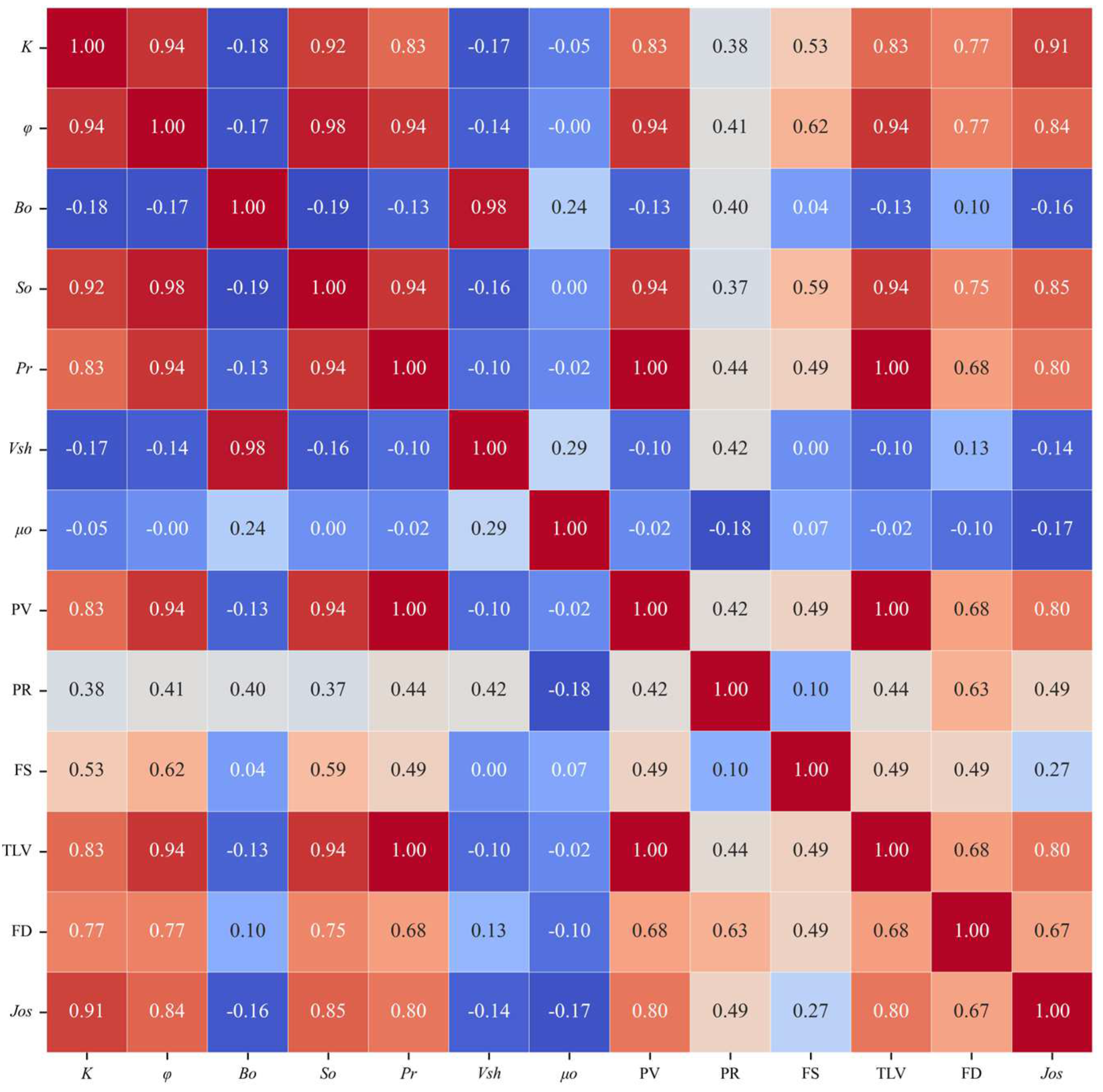
This paper utilized both Spearman’s correlation coefficient and random forest algorithms to identify and rank the main controlling factors affecting production from seven geological and five engineering factors in deep and ultra-deep offshore tight oil reservoirs. These factors were ranked based on their relative impact on productivity. The results of the two analysis methods are shown in Figure 2 and

Table 2. Random forest analysis correlation of productivity influence parameters.

Factors	K	φ	Bo	So	Pr	Vsh	μo	PV	PR	FS	TLV	FD
Correlation	0.92	0.87	−0.2	0.83	0.81	−0.2	−0.2	0.82	0.54	0.25	0.76	0.63

.

In this paper, the results from two methods—random forest and Spearman correlation coefficient—are used to identify the eight main controlling factors affecting the productivity of tight oil reservoirs in the WZ block. The screening results of the main control factors affecting the final production productivity are ranked as follows: K > φ > S_o > PV > P_r > TLV > FD > PR.

2.2.4. Data Normalization

Max-Min normalization [26] is employed for data preprocessing to map data with varying dimensions and units to a unified scale. This method preserves the relationships within the original data and is the simplest approach to eliminate the effects of differing dimensions and value ranges. The formula is defined as:

$$X^{\ast }={\displaystyle \frac{X_i-X_{min}}{X_{max}-X_{min}}}$$

(3)

where $X_i$ is the original data point; $X_{\mathit{min}}$ is the minimum; $X_{\mathit{max}}$ is the maximum; and $X^{\ast }$ is the normalized data point.

2.3. Construction of PSO-BP Prediction Model

2.3.1. Back Propagation (BP) Neural Network

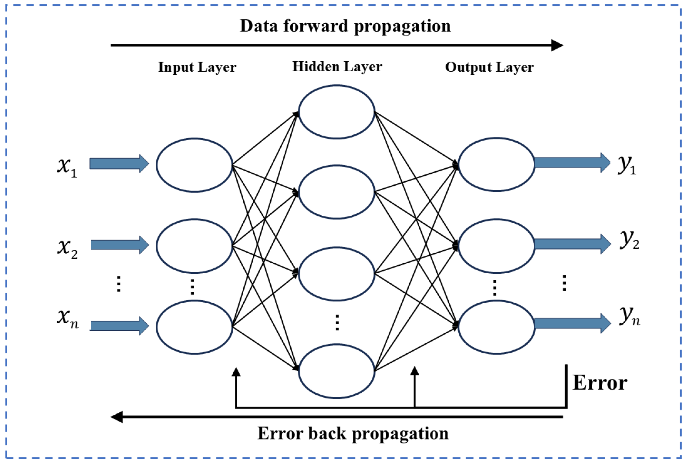
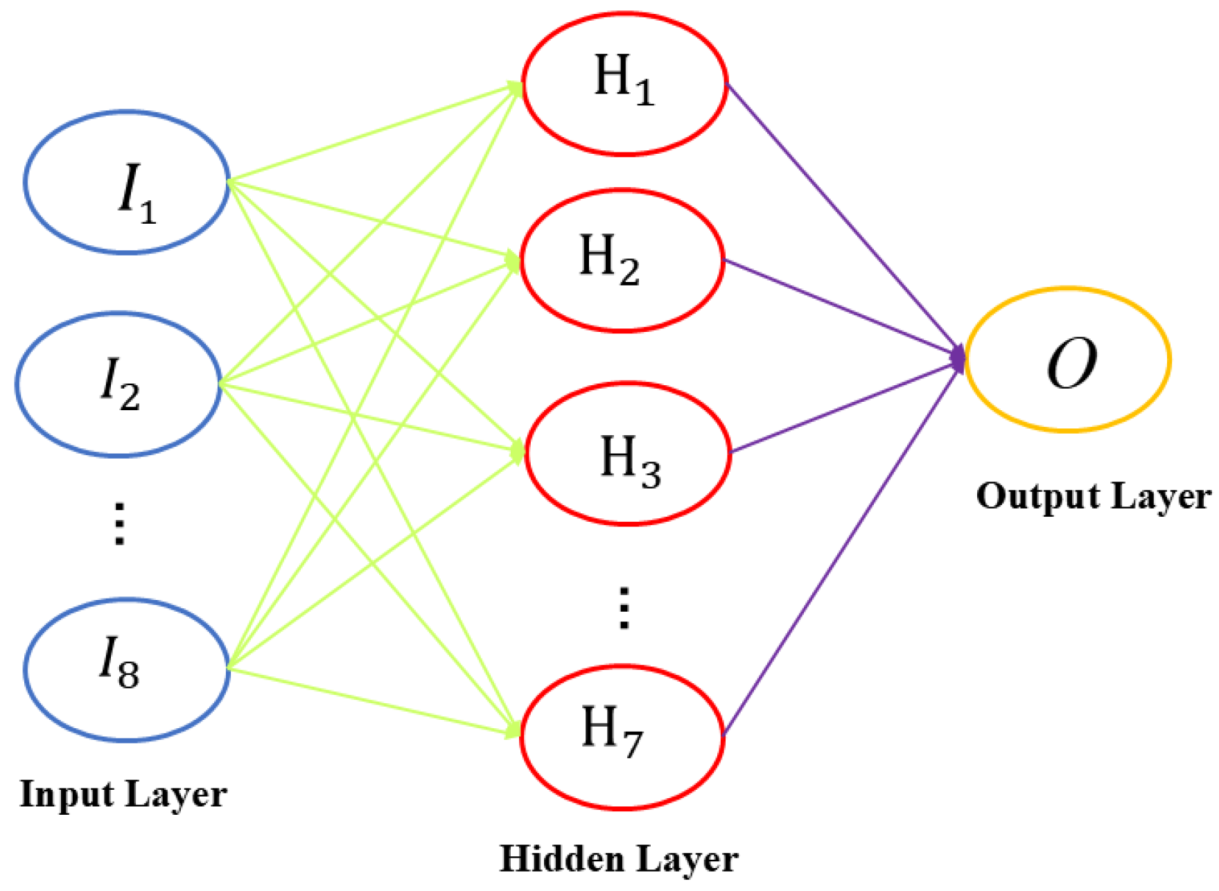
The BP neural network is a multi-layer feedforward network that utilizes error back propagation. It possesses strong nonlinear fitting and generalization abilities, making it capable of handling high-dimensional data and complex nonlinear relationships. Figure 3 illustrates the network structure of the model. Initially, the signal is transmitted forward from the input layer to the output layer, with each layer influencing only the subsequent layer. If the expected result is not achieved, it is compared with the actual output, and the resulting error is propagated backward. The weights and thresholds of the network are continuously adjusted through error backpropagation.

The basic process of constructing BP neural network is as follows:

$I$ number of input layer neurons; $H$ number of hidden layer neurons; $O$ number of output layer neurons; $w_{IH}$ input layer weight; $w_{HO}$ hidden layer weight; $a_j$ input layer bias; $c_k$ hidden layer bias; $\alpha$ learning rate; and $Y_k$ true value.

In the first step, the BP neural network is initialized by setting important parameters. These parameters include the number of network layers, the selection of activation functions, and the initial weights and biases of the network.

In the second step, the hidden layer output $Hid{e}_j$ formula is defined as:

$$Hid{e}_j=f\left({\displaystyle \sum _{i=1}^I{w}_{IH}{x}_i+a_j}\right)$$

(4)

In the third step, the output layer output $Ou{t}_k$ formula is defined as:

$$Ou{t}_k={\displaystyle \sum _{j=1}^{H}Hid{e}_j{w}_{HO}+c_k}$$

(5)

In the fourth step, the error formula is defined as:

$$Error={\displaystyle \frac{1}{2}}{\displaystyle \sum _k^O}{\left(Y_k-Ou{t}_k\right)}^2$$

(6)

In the fifth step, error back propagation, the network weights and biases are adjusted, and the formula is defined as:

$$w_{IH}=w_{IH}+\alpha Hid{e}_j\left(1-Hid{e}_j\right)x_i{\displaystyle \sum _{k=1}^O{w}_{HO}(Y_k-Ou{t}_k)}$$

(7)

$$w_{HO}=w_{HO}+\alpha Hid{e}_j\left(Y_k-Ou{t}_k\right)$$

(8)

$$c_k=c_k+\alpha (Y_K-Ou{t}_k)$$

(9)

2.3.2. Particle Swarm Optimization (PSO)

The particle swarm optimization (PSO) algorithm is a swarm intelligence-based search algorithm suitable for nonlinear function optimization in multidimensional spaces. The algorithm operates by randomly generating a swarm of particles within the space. These particles are evaluated on the basis of a fitness value determined by the objective function and move continuously through the space with a certain velocity. The algorithm begins by generating random particles, each of which is considered a potential solution. These particles traverse the solution space, forming a population, and achieve global optimization through multiple iterations. In each iteration, the individual optimal value $P_{best}$ and the group optimal value $g_{best}$ are obtained by comparing the fitness values of each particle, and the velocity and position of the particles are updated according to the positions of $P_{best}$ and $g_{best}$. The speed and position update formula is defined as:

$$v_{id}^{\left(k\right)}=\omega v_{id}^{\left(k-1\right)}+c_1{r}_1\left[P_{id}-x_{id}^{\left(k-1\right)}\right]+c_2{r}_2\left[g_{id}-x_{id}^{\left(k-1\right)}\right]$$

(10)

$$x_{id}^{\left(k\right)}=x_{id}^{\left(k-1\right)}+v_{id}^{\left(k\right)}$$

(11)

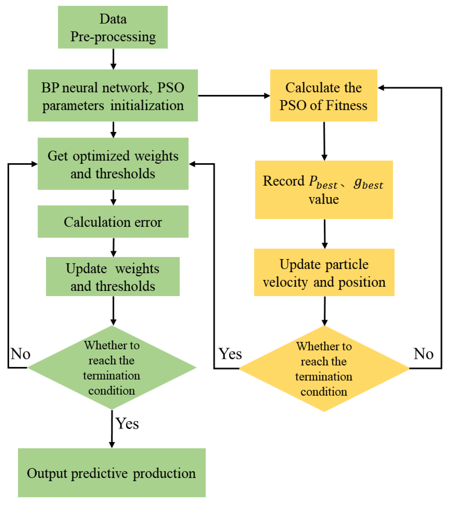
In the PSO algorithm, the parameter settings of inertia weight and $C_1$, $C_2$ acceleration factor have an essential influence on the performance of the algorithm. Increasing the $\omega$ value can improve the global search ability of the algorithm; otherwise, it can enhance the local search ability. Therefore, when $C_1$ is small and $C_2$ is large, the algorithm has better local search ability. The iterative process of PSO algorithm optimization is shown in Figure 4.

2.3.3. Construction of PSO-BP Neural Network

The fundamental principle of the BP neural network is to minimize the mean squared error between the expected and actual output values using gradient descent. This approach is highly dependent on the initial weights and thresholds and is prone to issues such as falling into local optima and slow convergence. To address these issues, this paper employs particle swarm optimization (PSO) to enhance the BP neural network, resulting in the construction of the PSO-BP neural network. The PSO-BP neural network utilizes the PSO algorithm to optimize the weights and biases of the BP network, thereby improving the network’s convergence speed and prediction accuracy. The flow of the optimization algorithm is shown in Figure 4.

Before the sample dataset is used for model training, data preprocessing must be performed, which includes handling missing values, detecting outliers, and normalizing the dataset to eliminate the influence of different value ranges and dimensions.

In the first step, the architecture of the BP network is initialized and the initial values are set for the connection weights and biases of the network.

In the second step, the PSO parameters, including the size of the population, the learning factor, the maximum number of iterations, and the position and speed of each particle, are initialized. The fitness function is set to the MSE of the BP network prediction value and the fitness function is used to find the fitness value of each particle.

In the third step, according to $P_{best}$ and $g_{best}$, the speed and position of each particle are updated to optimize the network parameters. The evaluation is repeated and the particles are updated.

In the fourth step, the optimal weight and bias parameters found by the PSO algorithm are set to the BP network, and the optimized BP network is used to predict the new input data. The model’s performance is evaluated by comparing the predicted results with the actual outcomes.

2.3.4. Model Parameter Settings

Designing the PSO-BP model requires careful consideration of the network model’s key parameters. Different parameter combinations directly affect the prediction accuracy and speed of the productivity model. For example, an excessive number of hidden layers can cause the neural network to overfit. Conversely, a model with too few hidden layers may reduce the prediction accuracy and fail to adequately capture the problem’s complexity, leading to unsatisfactory results. Therefore, selecting a relatively optimal neural network structure through multiple experiments is necessary.

The classical three-layer neural network structure is used to construct the productivity prediction model. Taking the eight main control factors of capacity influence selected above as input parameters, the input layer neurons ($I$) are 8, the specific oil production index is used as the output parameter, and the output layer neuron ($O$) is set to 1. The empirical formula of $H$ is defined as:

$$H=\sqrt{I+O}+b$$

(12)

where $b$ is a constant between 1 and 10; therefore, the value range of $H$ is 4~13.

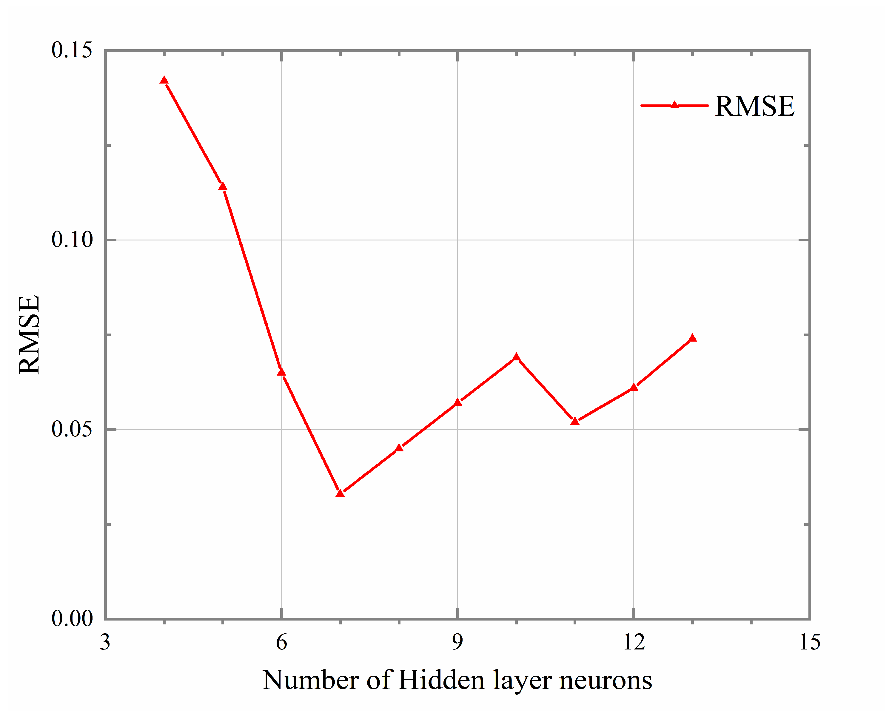
The experimental results are shown in Figure 5. After numerous experiments, it was found that, when the number of hidden layer neurons is 7, the RMSE of the test set is minimized. Therefore, the number of hidden layer nodes was finalized at seven. Therefore, the BP model structure finally constructed in this paper is shown in Figure 6.

The parameter settings of the PSO-BP model are shown in

Table 3. PSO-BP neural network model main parameter settings.

Parameter	Value
I	8
H	7
O	1
Hidden layer activation function	Tansig
Output layer activation function	Purelin
Training function	Trainlm
C1	[0,1.5]
C2	[1.5,2]
Maximum number of iterations	2000
Population size	30
Learning rate	0.0001
Expected error	0.0001
ω	[0.3,0.9]

.

2.3.5. Model Evaluation Performance Measures

This paper utilizes three widely recognized model evaluation metrics: RMSE, MAE, and R². These metrics are employed to evaluate the predictive performance of the models [26]. The formulas are as follows:

$$RMSE=\sqrt{{\displaystyle \frac{1}{n}}{\displaystyle \sum _{i=1}^n{(y_i-\widehat{y_i})}^2}}$$

(13)

$$MAE={\displaystyle \frac{1}{n}}{\displaystyle \sum _{i=1}^n\left|y_i-\widehat{y_i}\right|}$$

(14)

$$R^2={\displaystyle \frac{{\displaystyle {\sum }_{i=1}^n{(\widehat{y_i}-\overline{y_i})}^2}}{{\displaystyle {\sum }_{i=1}^n{(y_i-\overline{y_i})}^2}}}$$

(15)

3. Field Application

The tight oil reservoir in the Weizhou Block is located in the central region of the Weixinan Sag, within the Beibuwan Basin in the South China Sea. The basin includes three depressions and two uplifts, which are classified as secondary tectonic units. The primary oil-bearing intervals in the study area are predominantly located in the Liushagang Formation. This formation has an average porosity of 14.3% and an average permeability of 0.87 mD, classifying the reservoir as tight oil.

To ensure the accuracy and reliability of the tight reservoir productivity prediction model, 145 development wells from the WZ block in the Beibu Gulf area were used as training and validation samples. Of these, 116 wells were randomly selected to form the training set, while the remaining 29 wells constituted the test set. The training set is used to construct the capacity prediction model, including training and parameter adjustment, whereas the test set data are not involved in model training. The main function of the test set is to evaluate the model’s generalization ability (its adaptability to unknown data) after the model has been established, testing the authenticity and applicability of the machine-learning capacity prediction model.

To mitigate the impact of random division of the training and test sets and enhance the stability and generalization ability of the model, this study conducts multiple experiments and averages the predictions to determine the final result. The specific implementation steps are outlined below.

In the first step, the dataset is randomly divided into training (80%) and test sets (20%). This process is repeated 20 times.

In the second step, after each division, the BP neural network undergoes training with the training set, followed by prediction with the test set.

In the third step, the prediction results of each experimental test set are recorded and then converted to actual prediction values via the antinormalization formula. The formula is defined as:

$$X_i=X^{\ast }(X_{\mathit{max}}-X_{\mathit{min}})+X_{\mathit{min}}$$

(16)

In the fourth step, the final prediction results take the average of 20 experimental prediction results.

3.1. Prediction Results of the Model

In this paper, PSO-BP is used to construct a productivity prediction model for tight reservoirs in the WZ block. The model is trained on the data of 116 wells in the training set and the 8 main controlling factors of productivity.

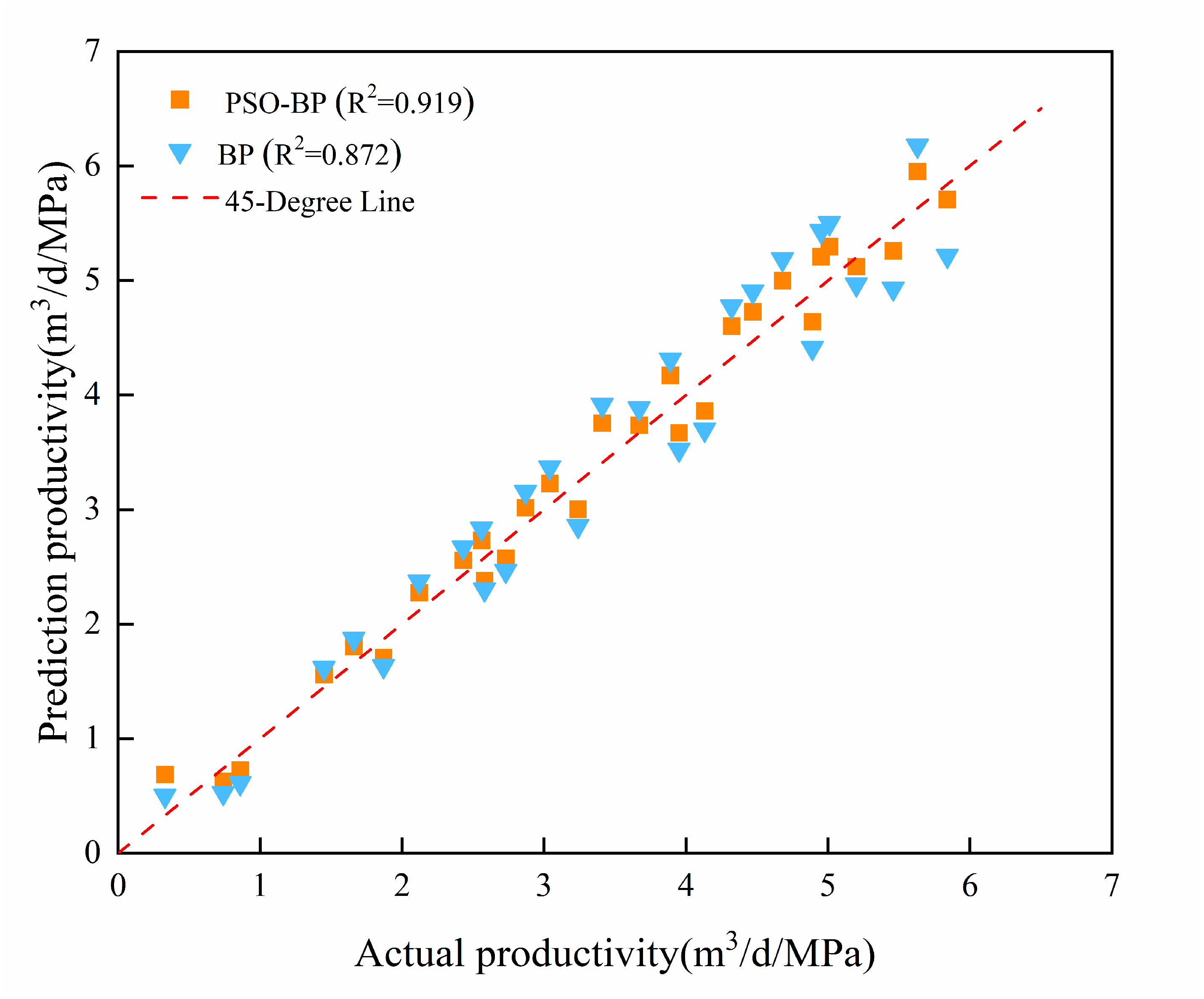
The training set data are used to construct two capacity prediction models: PSO-BP and BP. The prediction results are shown in Figure 7, and the evaluation metrics for both models are shown in

Table 4. Comparison of results of PSO-BP and BP.

Model	PSO-BP	BP
Running time (t/s)	17.84	22.89
RMSE	0.032	0.041
MAE	1.209	1.478
R2	0.919	0.872

. The evaluation metrics for the PSO-BP model indicate an RMSE of 0.032, an MAE of 1.209, and an R² value of 0.919, demonstrating a small error between the predicted values and actual production capacity and high accuracy.

As shown in Figure 7, compared with the BP model, the PSO-BP model is closer to the actual productivity and R² is increased by 0.047. In this paper, the global optimization ability of particle swarm optimization is used to optimize the threshold and weight of BP neural network. Therefore, the PSO-BP model demonstrates superior accuracy, faster computational speed, and enhanced generalization ability.

3.2. Comparison of Different Productivity Prediction Models

Utilizing the aforementioned BP neural network optimized through particle swarm optimization (PSO-BP), a productivity prediction model for offshore deep and ultra-deep tight reservoirs is developed. To further validate the rationality and practicality of this model, two traditional productivity prediction models, empirical formulas and numerical simulations, are used. The empirical formula uses the radial flow equation, which is as follows:

$$q={\displaystyle \frac{0.00708\cdot k\cdot h\cdot \left(\Delta P\right)}{\mu \cdot \ln \left(\frac{r_e}{r_w}\right)}}$$

(17)

Numerical simulation is conducted using the reservoir simulation software tNavigator (version 24.1) to predict productivity.

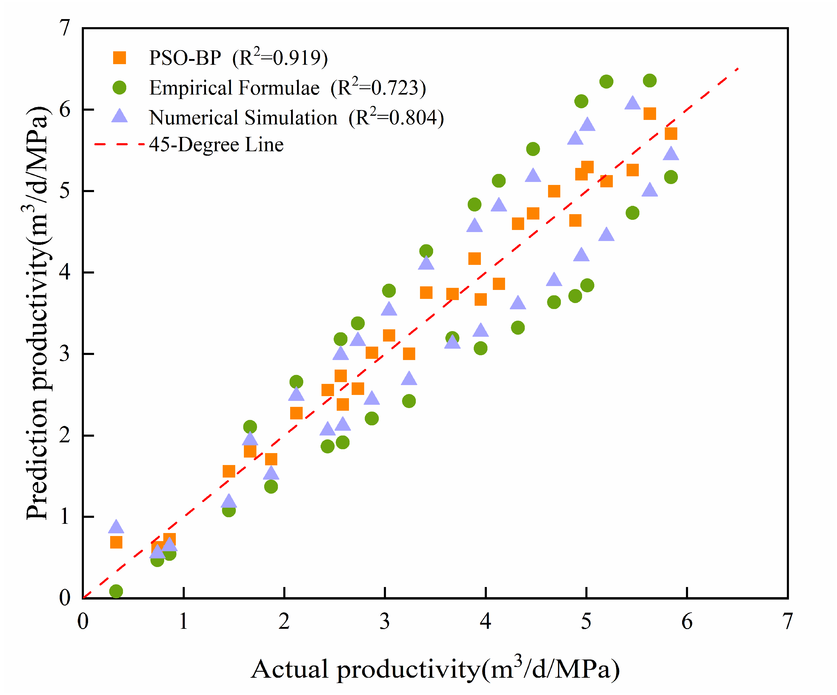
The data of 29 wells in the test set are used to predict and compare the prediction results of different models. The prediction results of the different models on the test set are shown in Figure 8.

As shown in Figure 8, among the three productivity prediction models, the PSO-BP model generally results in the smallest errors, followed by numerical simulation, whereas the empirical productivity formula results in a larger prediction error.

The different model results for the test set data are shown in

Table 5. Comparison of results of test set data.

Model	PSO-BP	Numerical Simulation	Empirical Formulae
Running time (t/s)	17.841	1500.182	60
RMSE	0.032	0.045	0.063
MAE	1.209	1.670	2.240
R2	0.919	0.804	0.723

.

As shown in Table 5, the PSO-BP model proposed in this paper has the smallest error, highest accuracy, and fastest running speed. This finding demonstrates that, for offshore deep and ultra-deep tight reservoirs, the PSO-BP productivity prediction model can more effectively address the complex nonlinear relationships among various productivity-influencing factors than traditional prediction methods, thereby greatly improving the accuracy and effectiveness of productivity predictions in tight reservoirs.

4. Discussion

Traditional productivity prediction methods (empirical formulas and numerical simulations) for tight reservoirs suffer from low accuracy. This discrepancy arises because empirical formulas are complex mathematical constructs based on seepage mechanics. During their development, many factors affecting productivity, such as engineering considerations, are neglected, and idealized assumptions are made when using empirical formulas for prediction. The numerical simulation method relies on a reservoir model and basic seepage theory, which are established through computer simulations. While the accuracy of the modeling parameters is high, the simulation process is cumbersome. However, tight reservoirs differ from conventional ones; the seepage mechanisms are extremely complex, rendering basic seepage theory less applicable. Additionally, data acquisition is challenging, and some data are incomplete, leading to significant deviations in model predictions.

This paper proposes a productivity prediction model (PSO-BP), which serves as a crucial tool for evaluating and predicting the production of offshore deep and ultra-deep tight reservoirs. Compared with traditional productivity prediction methods, this model comprehensively accounts for the impact of both geological and engineering factors on productivity and integrates mathematical statistics and machine learning methods to significantly enhance prediction accuracy for tight oil reservoirs.

However, the PSO-BP model has specific applicability and certain limitations. The primary factors influencing the productivity of tight reservoirs vary across different blocks. For instance, the model performs better in the WZ block tight oil reservoir; however, its effectiveness in other oil fields, where geological and engineering factors differ, is uncertain. This may be due to the model’s selection of factors that do not align with the actual production conditions in other oil fields, resulting in reduced prediction accuracy. Therefore, when addressing various types of tight oil reservoirs, it is necessary to adjust the model parameters to achieve accurate productivity predictions.

5. Conclusions

The conclusions obtained from this work are as follows:

(1)

This paper adopts an integrated methodology that uses both Spearman correlation coefficient analysis and random forest algorithms to evaluate the impacts of geological and engineering factors on productivity. The analysis identified eight main factors that influence productivity. The ranking results of these main control factors affecting final productivity are as follows: K > φ > S_o > PV > P_r > TLV > FD > PR.

(2)

This paper utilizes primary factors influencing tight reservoir productivity to develop a productivity prediction model for offshore deep and ultra-deep tight reservoirs, employing a BP neural network optimized with particle swarm optimization (PSO-BP). The model demonstrates superior accuracy and faster prediction speeds for oil well productivity. Error assessment of the model reveals favorable performance, with a root mean square error (RMSE) of 0.032, a mean absolute error (MAE) of 1.209, and an R² value of 0.919. In comparison to traditional productivity prediction methods (empirical formulas and numerical simulations), the PSO-BP model avoids many limitations and assumptions, more effectively addresses the complex nonlinear relationships among productivity-influencing factors, and improves prediction accuracy for tight reservoirs.

(3)

In this paper, the PSO-BP model thoroughly incorporates the impact of both geological and engineering factors on productivity and combines mathematical statistics and machine learning methods to construct a productivity prediction model. Field applications demonstrate that the calculation results of the PSO-BP model closely align with actual oil well production, making it practical and valuable for guiding the design of tight oil reservoirs and offering potential economic benefits for oilfield development.

(4)

Artificial neural networks, such as the MLP, CNN, and RNN, offer significant value in predicting tight reservoir productivity. Depending on the task requirements, data types, and prediction objectives, the most suitable algorithm is chosen to construct the productivity prediction model. These models can effectively increase the efficiency and accuracy of reservoir productivity predictions. As data continue to be enriched and algorithms are optimized, both the prediction accuracy and application potential are expected to improve further.