
Research on Flexible Braking Control of a Crawler Crane during the Free-Fall Hook Process

Abstract
1. Introduction
2. Modeling and Analysis of Free-Fall Hook Systems
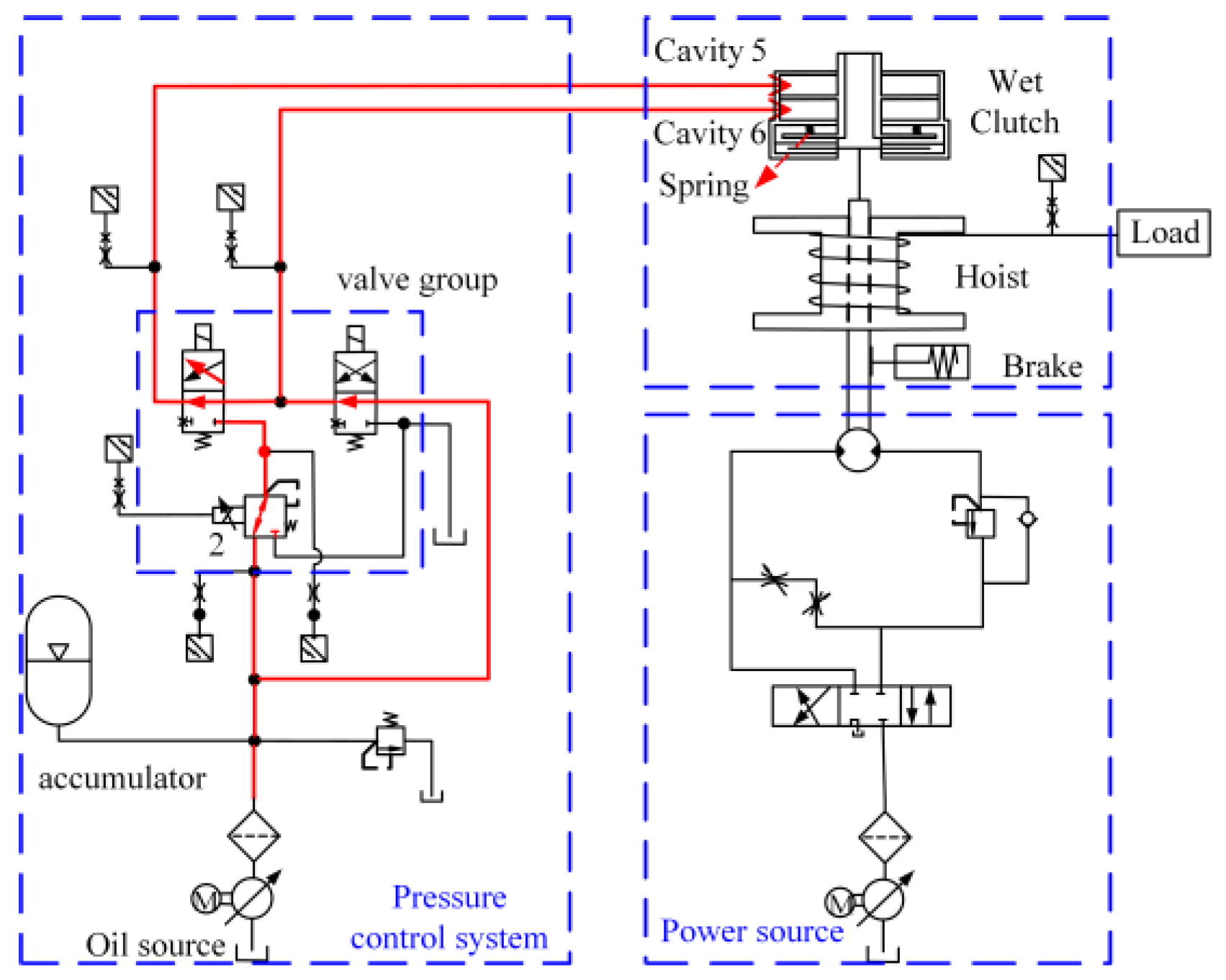
2.1. Composition and Working Principle of Free-Fall Hook Systems
2.2. Mathematical Modeling and Characterization
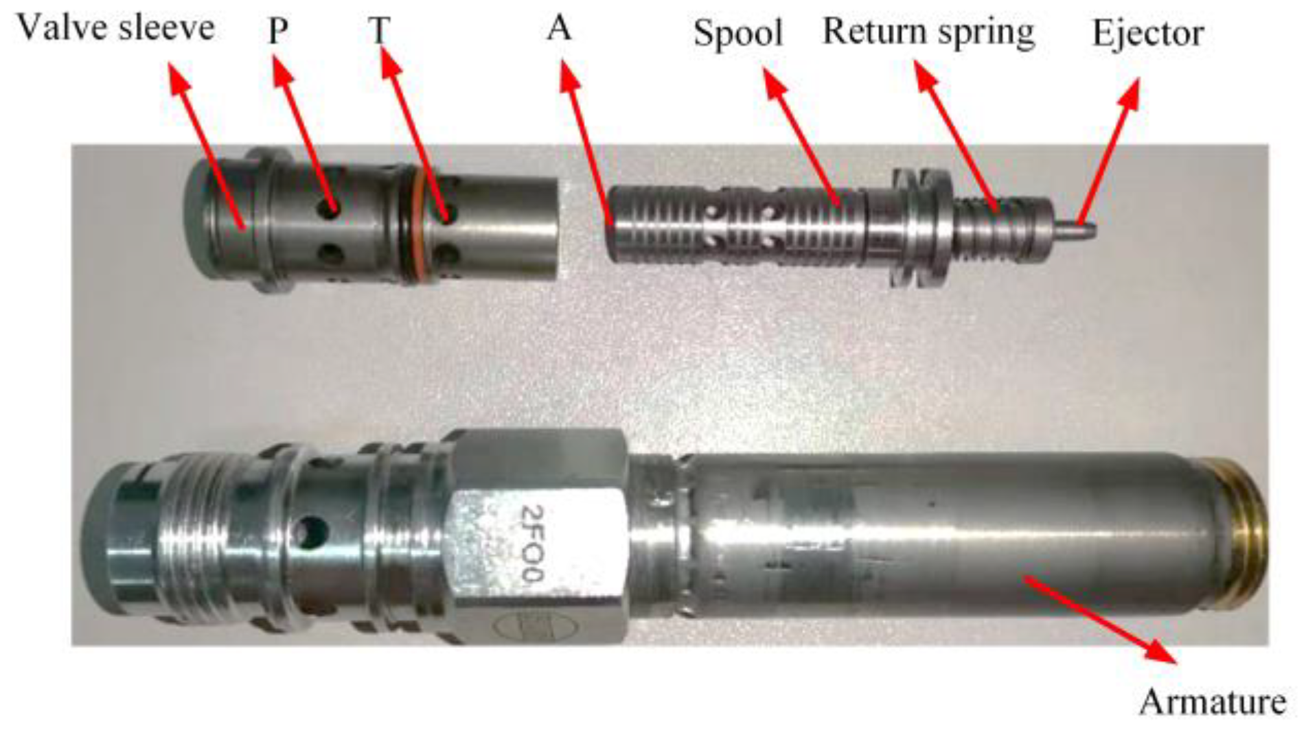
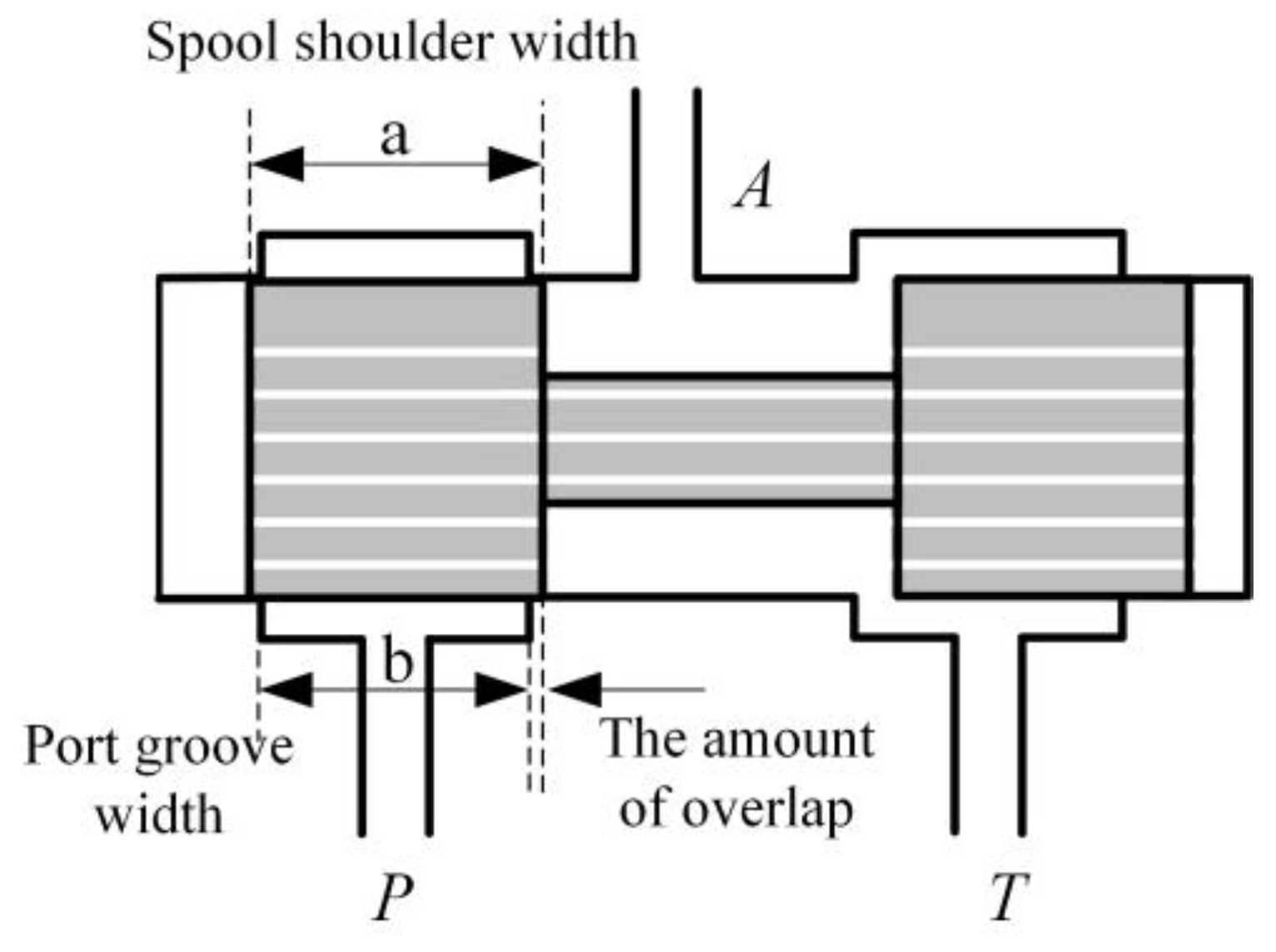
2.2.1. Model of a Proportional Pressure-Reducing Valve
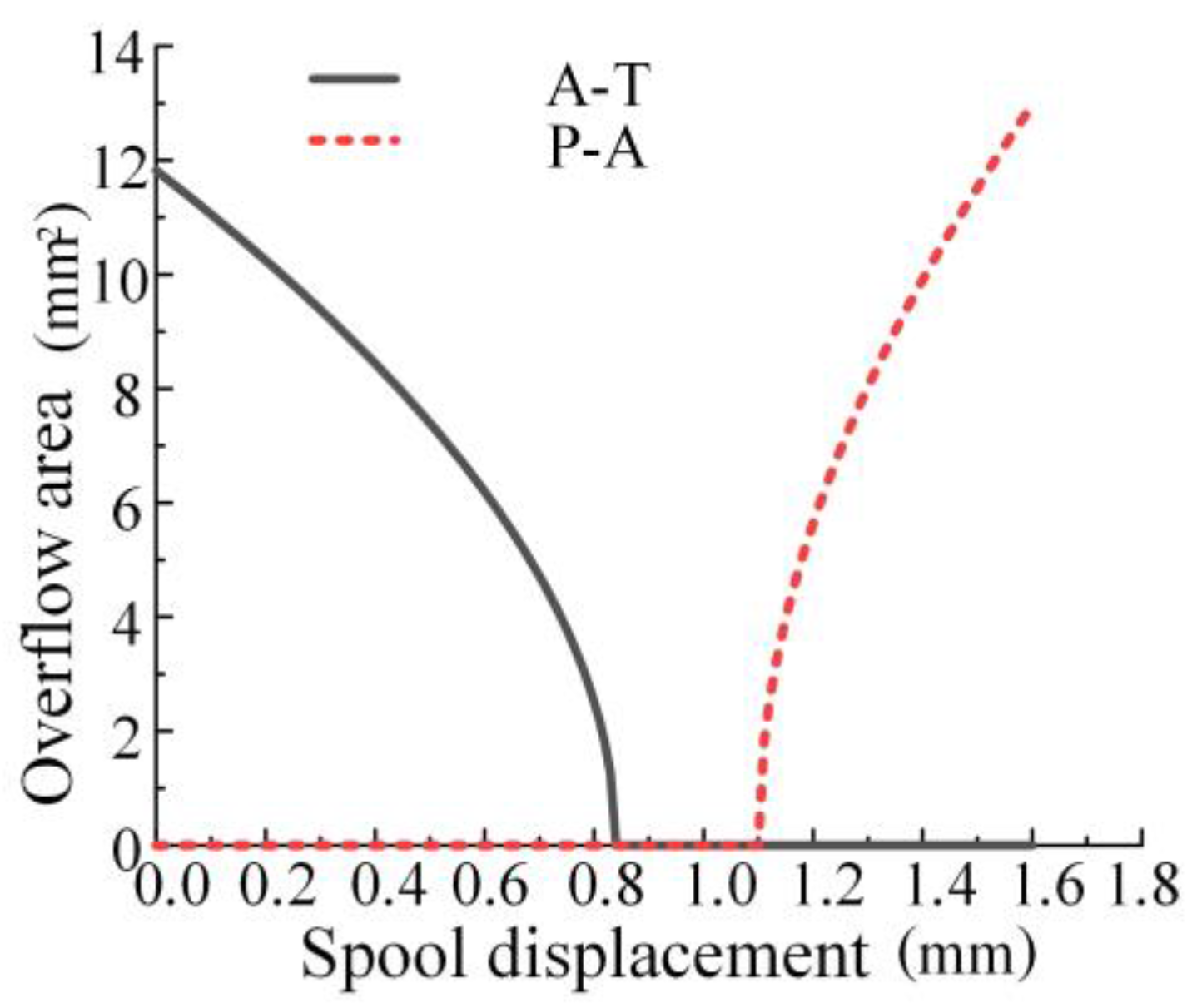
- Proportional Pressure-Reducing Valve Overflow Area Calculation
- 2.
- Spool force analysis of proportional pressure-reducing valves
2.2.2. Modeling of Free-Fall Hook Wet Clutches
2.2.3. Transfer Function of a Free-Fall Hook System
2.3. Nonlinear Characterization of a Free-Fall Hook System
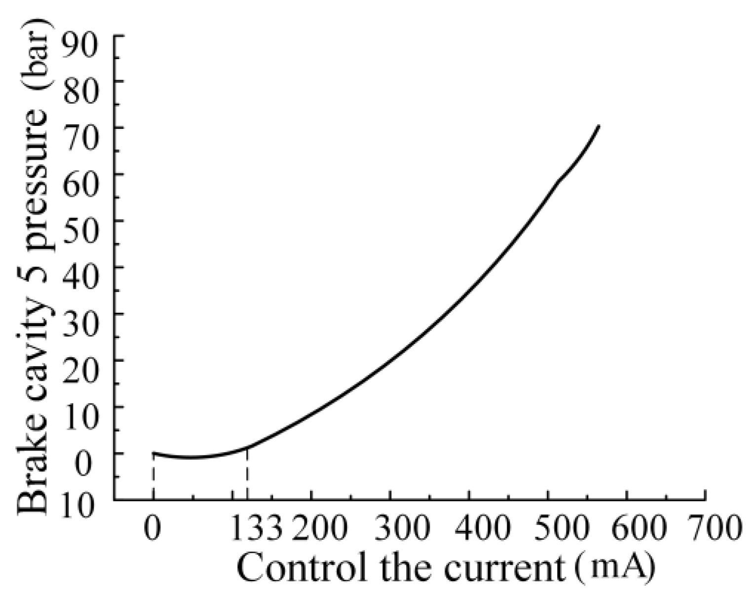
2.3.1. Analysis of System Pressure Dead Band Characteristics
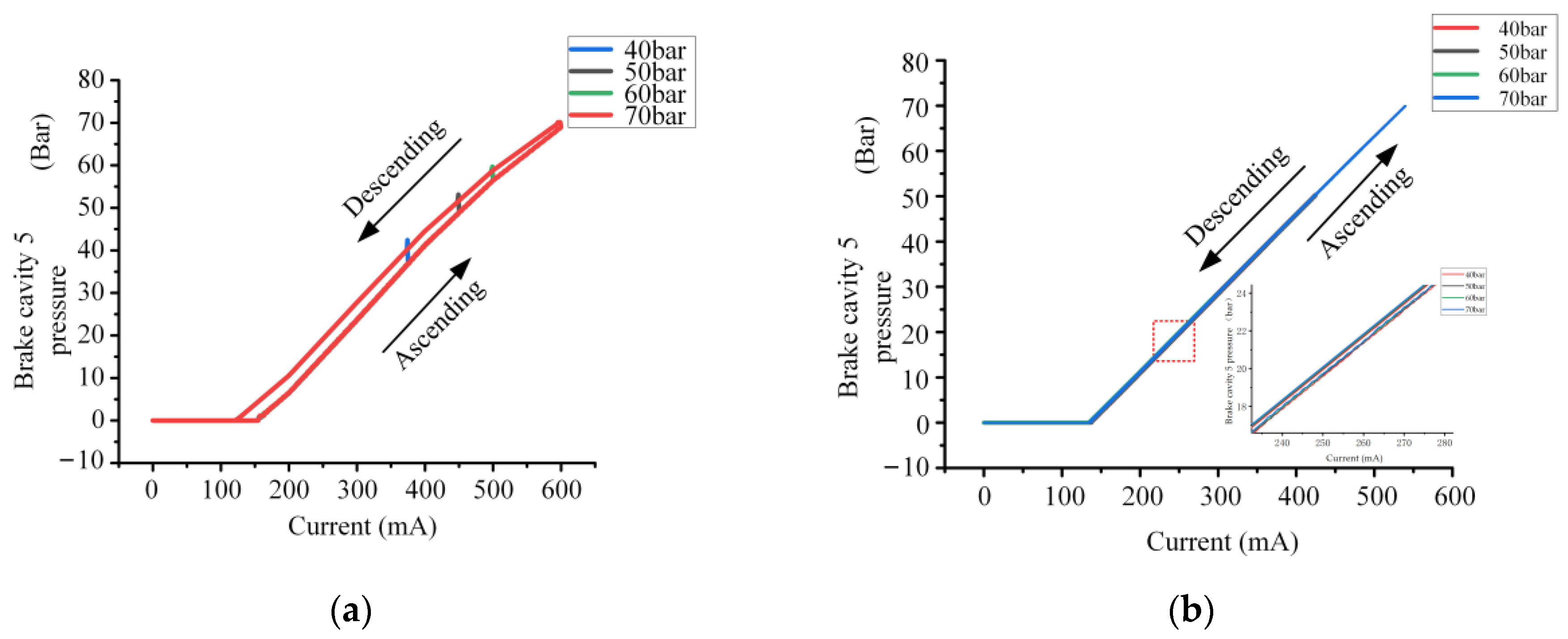
2.3.2. System Pressure Hysteresis
3. Research on the Control Strategy of the Free-Fall Hook System
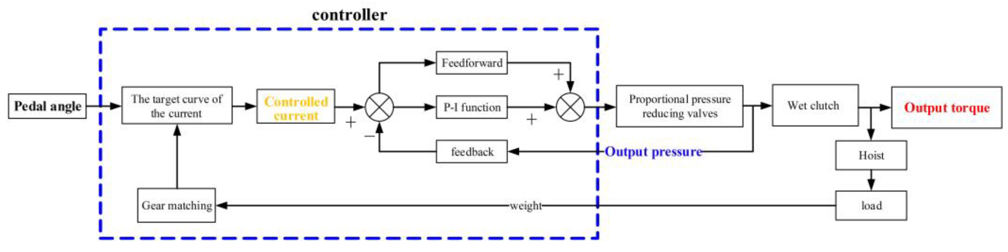
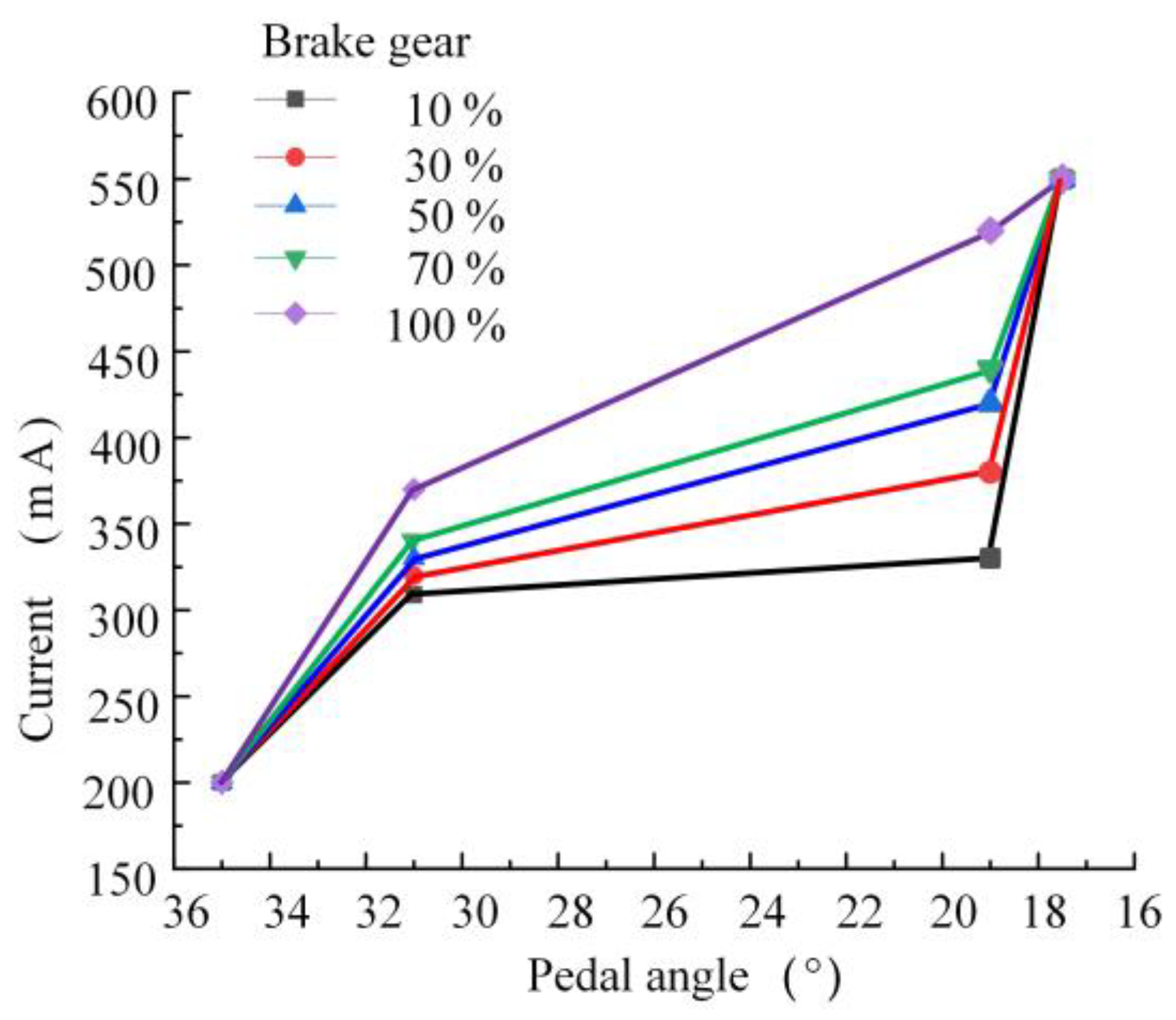
3.1. Automatic Braking Gear Matching Control Strategy
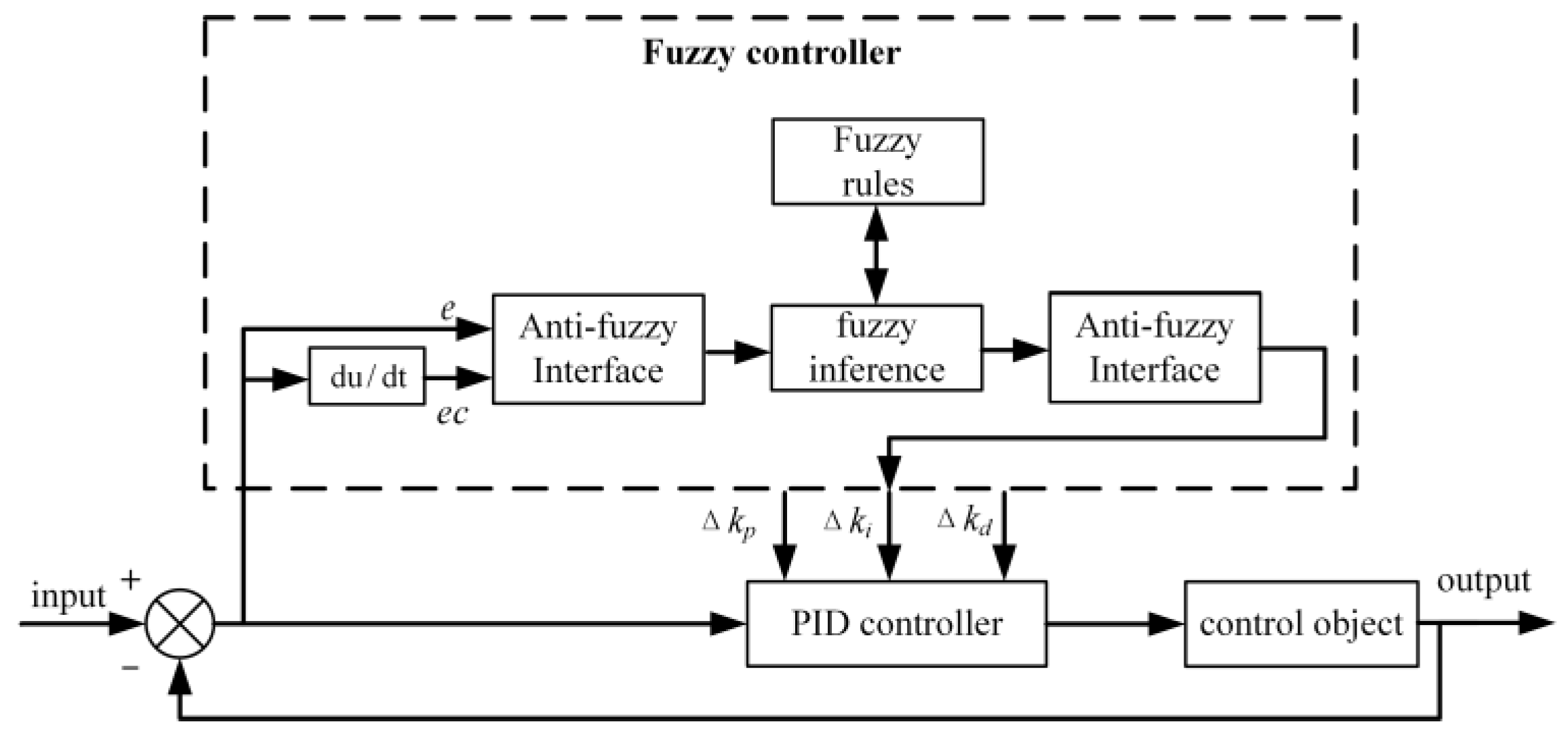
3.2. Fuzzy Controller Design
3.2.1. Define Inputs and Outputs
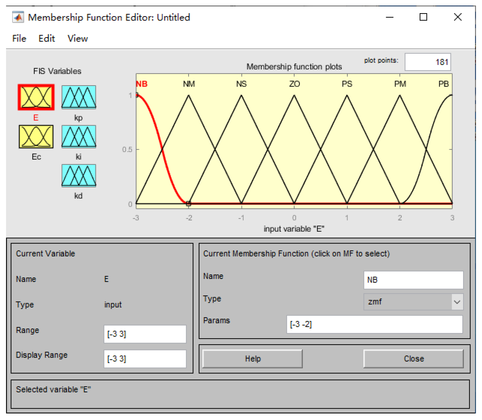
3.2.2. Determine the Affiliation Function
3.2.3. Determining the Fuzzy Rules
3.2.4. Fuzzy Reasoning
3.2.5. Defuzzification to Obtain the Controller
4. Simulation Verification of the Control Strategy of the Free-Fall Hook System
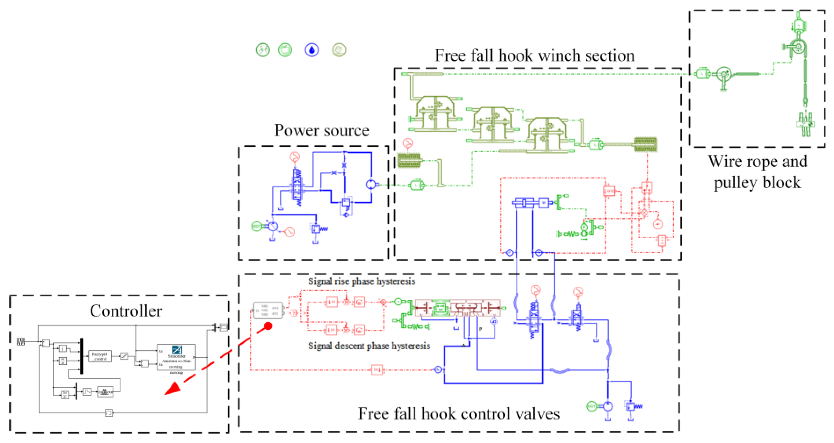
AMESim and MATLAB Co-Simulation Platform
5. Experimental Study of the Flexible Control of the Free-Fall Hook System
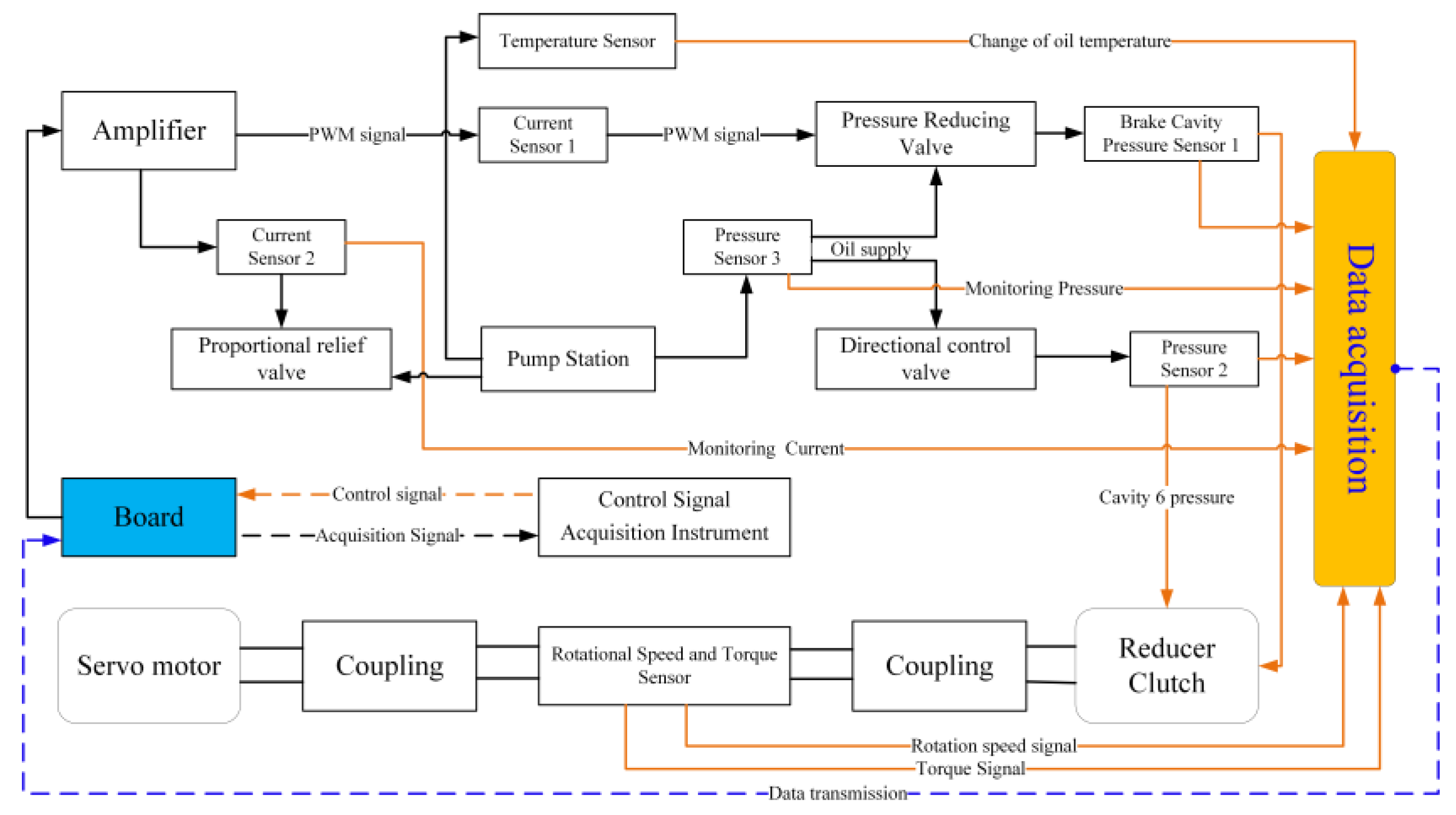
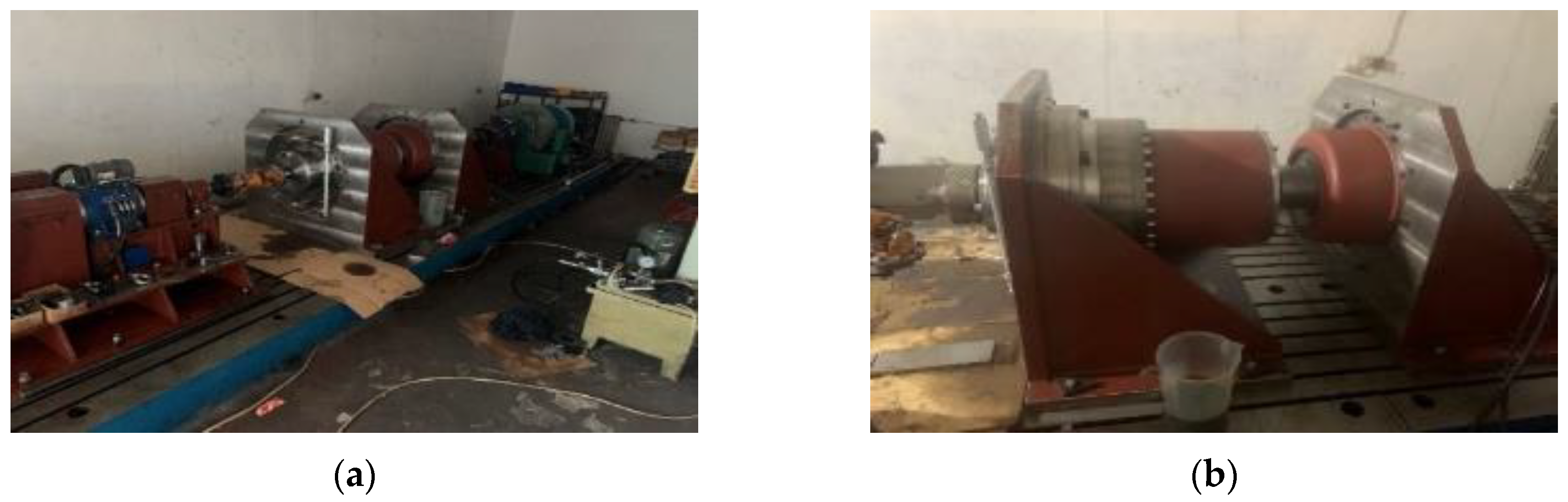
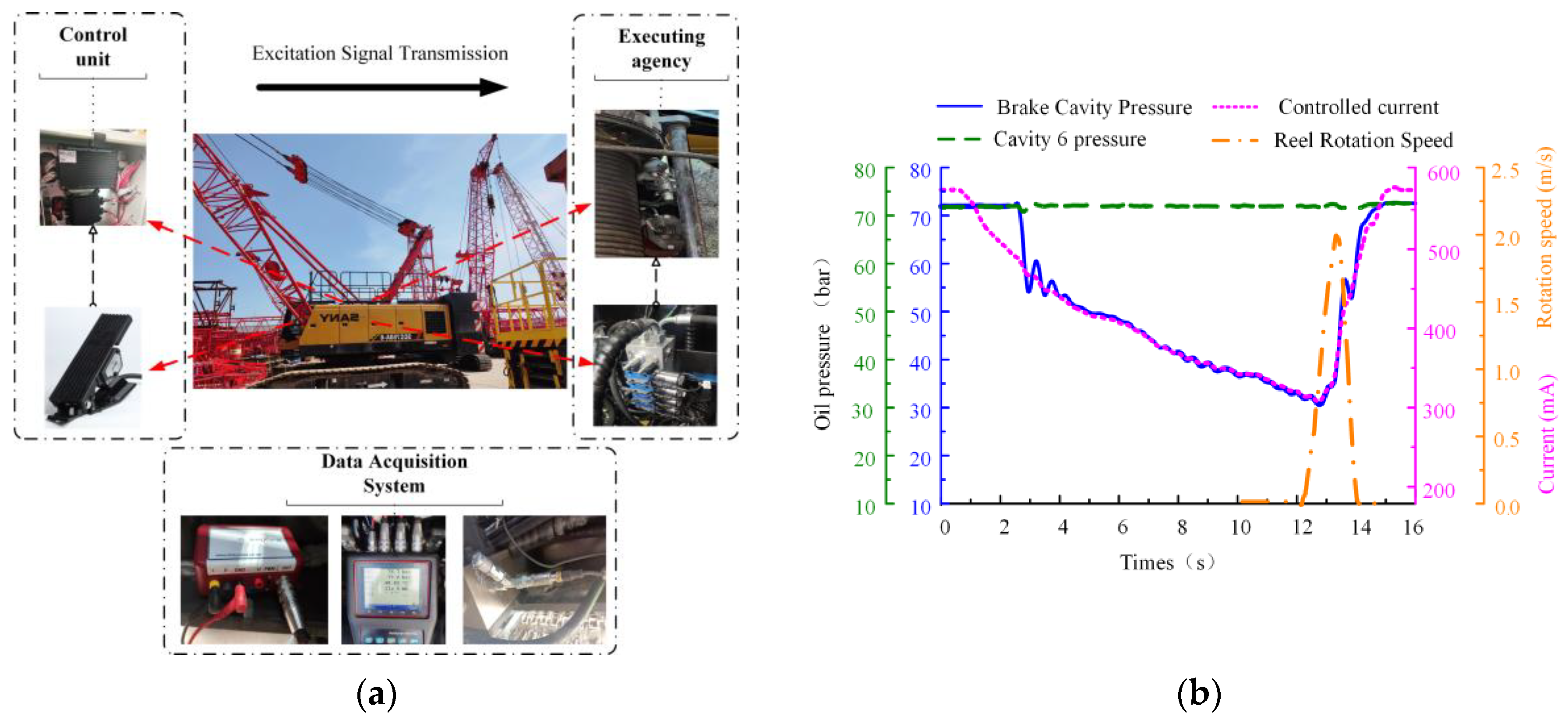
5.1. Experimental Bench Study
5.2. Analysis of the Free-Fall Hook Process
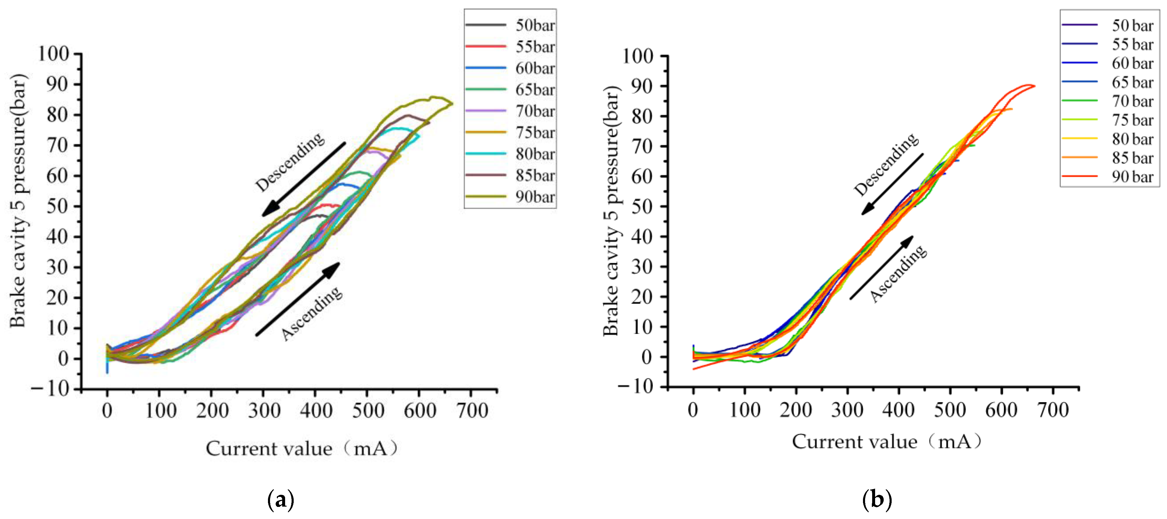
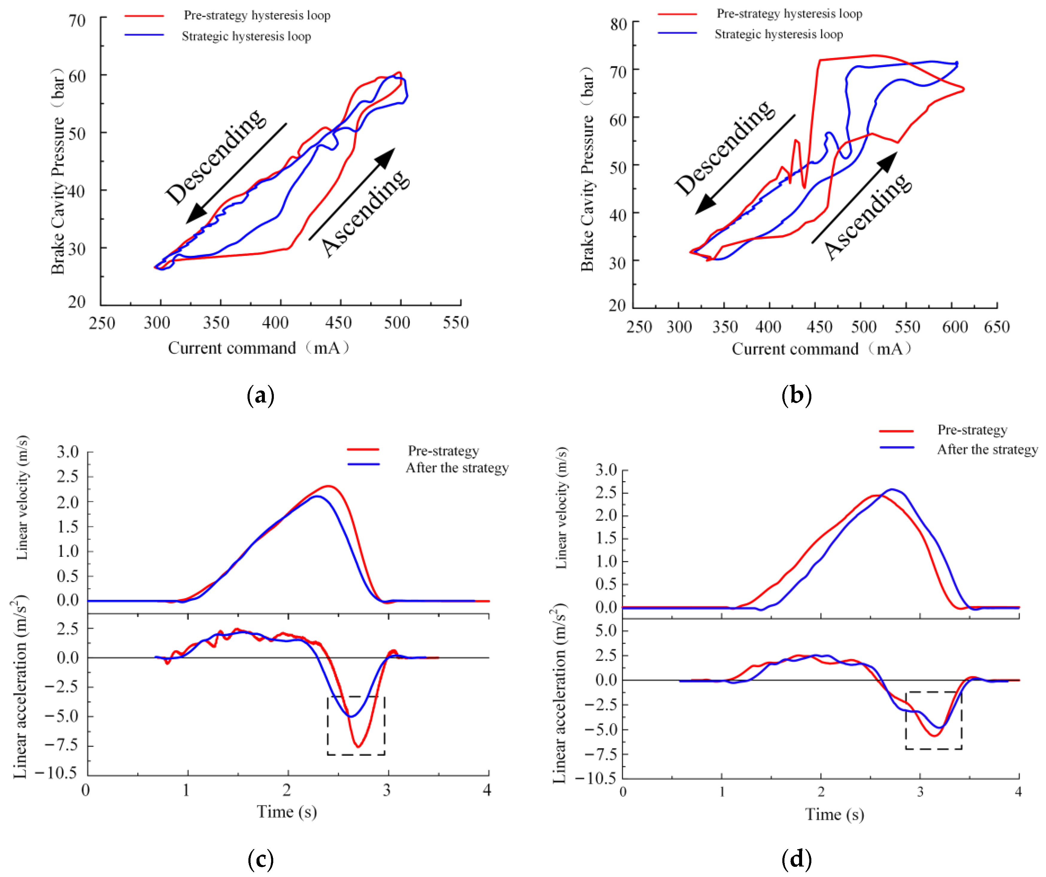
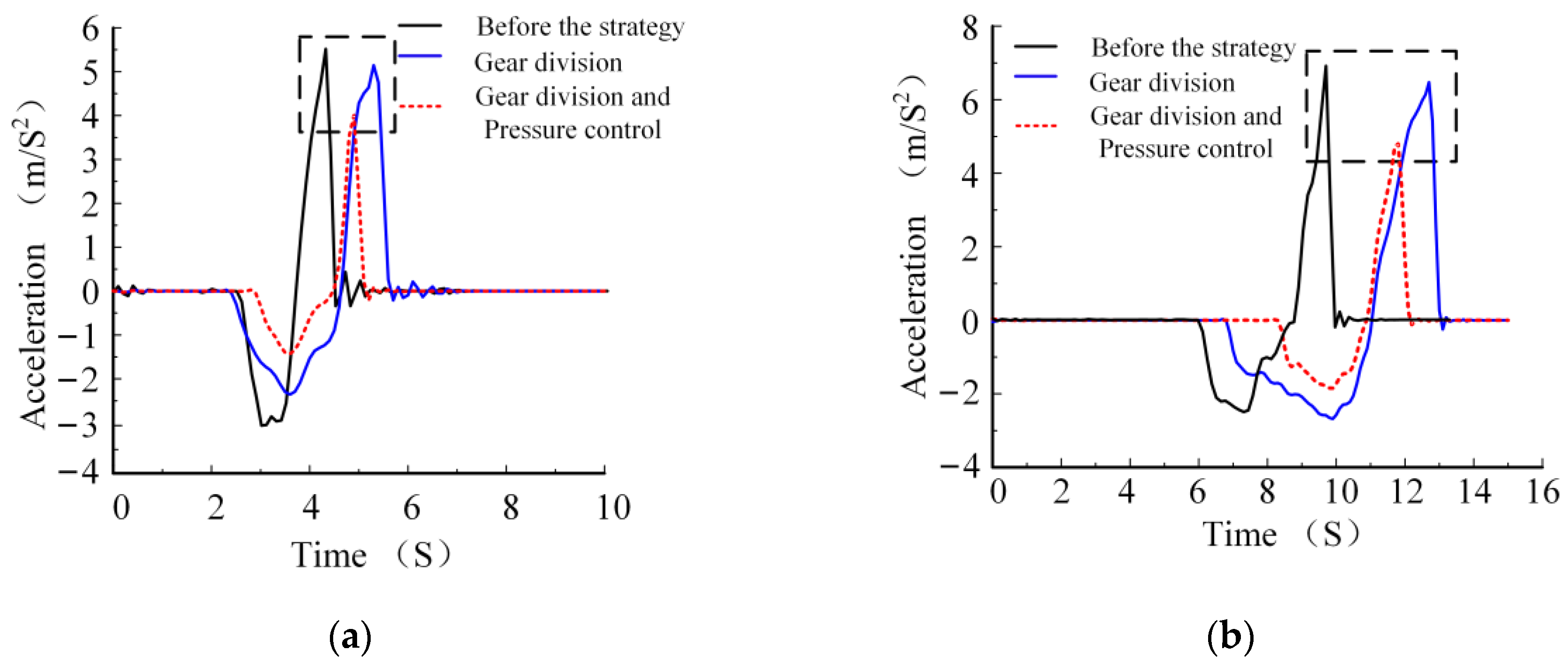
5.3. Analysis of the Hysteresis Loop and Braking Acceleration
6. Limitations and Future Work
7. Conclusions
- (1)
- For the free-falling hook system with large inertia and strong impact characteristics, the dead zone and hysteresis loop characteristics of the proportional decompression valve pressure output are obtained, and the control strategy of dividing the braking gears, assigning different current slopes at different stages, and automatically matching the mechanism of load weight, combined with the feed-forward and fuzzy PID pressure closed-loop, is proposed.
- (2)
- Based on the nested closed-loop control strategy in this paper, the system hysteresis loop is only 11%, which is more than 50% lower than before.
- (3)
- After using the control strategy, the maximum braking acceleration is reduced by 31.22% for a load of 6.44 tonnes and by 24.24% for a load of 10.44 tonnes, which significantly improves the flexible and smooth braking effect of a free-fall hook with a load.
Author Contributions
Funding
Data Availability Statement
Conflicts of Interest
References
- Shaikh, A. Lifting capacity enhancement of a crawler crane by improving stability. J. Theor. Appl. Mech. 2016, 54, 219–227. [Google Scholar] [CrossRef]
- Tuan, L.A.; Lee, S.-G. Modeling and advanced sliding mode controls of crawler cranes considering wire rope elasticity and complicated operations. Mech. Syst. Signal Process. 2018, 103, 250–263. [Google Scholar] [CrossRef]
- Muhammad, A.G.; Asif, M.; Shuai, L.; Jacek, O.; Ahmed, B.; Mohamed, A.-H. Decision support for hydraulic crane stabilization using combined loading and crane mat strength analysis. Autom. Constr. 2021, 131, 103884. [Google Scholar]
- Hao, H.; Ma, H. Optimizing Gearshift Control of Wet Dual Clutch Transmission. Mech. Sci. Technol. Aerosp. Eng. 2022, 41, 936–947. [Google Scholar]
- Yan, H.; Xu, S.; Tan, W.; Wu, J.; Zhang, Y. Study on dynamic engagement characteristics of friction clutch under input fluctuating speed. Mod. Manuf. Eng. 2021, 10, 33–39. [Google Scholar]
- Wu, B.; Qin, D.; Hu, J.; Wang, X.; Wang, Y.; Lv, H. Analysis of influencing factors and changing laws on friction behavior of wet clutch. Tribol. Int. 2021, 162, 107125. [Google Scholar] [CrossRef]
- Wang, C.; Qin, D.T.; Wu, B.Z.; Fang, H.S.; Cheng, K. Simulation and analysis of wet clutch engagement characteristics. J. Chong-Qing Univ. 2020, 43, 38–51. [Google Scholar]
- Heng, Z.; Heyan, L. Experimental Study on Attenuation Characteristics of Friction Torque Transferred by the Wet Multi-disc Clutch. J. Harbin Inst. Technol. 2018, 50, 94–102. [Google Scholar]
- Yang, C.; Wu, P.; Shang, X.; Wang, Z. Simulation and experimental study of engagement process with groove consideration. J. Zhejiang Univ. Eng. Sci. 2019, 53, 1225–1236. [Google Scholar]
- Meng, Q.; Tian, Z.; Zhao, C. Non-uniform contact characteristics of the friction disc during the initial period of a braking process. J. Mech. Sci. Technol. 2018, 32, 1261–1268. [Google Scholar]
- Fei, J.; Luo, W.; Huang, J.F.; Ouyang, H.; Xu, Z.; Yao, C. Effect of carbon fiber content on the friction and wear performance of paper-based friction materials. Tribol. Int. 2015, 87, 91–97. [Google Scholar] [CrossRef]
- Yu, L.; Ma, B.; Chen, M.; Li, H.; Ma, C.; Liu, J. Comparison of the Friction and Wear Characteristics between Copper and Paper Based Friction Materials. Materials 2019, 12, 2988. [Google Scholar] [CrossRef] [PubMed]
- Liu, Y.; Chen, M.; Yu, L.; Wang, L.; Feng, Y. Influence of Material Parameters on the Contact Pressure Characteristics of a Multi-Disc Clutch. Materials 2021, 14, 6391. [Google Scholar] [CrossRef] [PubMed]
- Padmanabhan, S.; Vinod Kumar, T.; Sendil Kumar, D.; Velmurugan, G.; Akshay Kumar, B.; Hitesh Sri Subramanyam, K. Investigation of structural and thermal analysis of clutch facings with different friction materials. Mater. Today Proc. 2023, 92, 98–105. [Google Scholar] [CrossRef]
- Bao, H.Y.; Xu, T.J.; Jin, G.H.; Huang, W. Analysis of Dynamic Engaged Characteristics of Wet Clutch in Variable Speed Transmission of a Helicopter. Processes 2020, 8, 1474. [Google Scholar] [CrossRef]
- Lu, K.; Wang, L.; Lu, Z.; Zhou, H.; Qian, J.; Zhao, Y. Sliding Mode Control for HMCVT Shifting Clutch Pressure Tracking Based on Expanded Observer. Trans. Chin. Soc. Agric. Mach. 2023, 54, 410–418. [Google Scholar]
- Kuang, J.K. Control of electro-hydraulic actuated clutch system based on nonlinear feed-forward controller. China J. Constr. Mach. 2022, 20, 199–204. [Google Scholar]
- Fu, S.; Gu, J.; Li, Z.; Mao, E.; Du, Y.; Zhu, Z. Pressure Control Method of Wet Clutch for PST of High-power Tractor Based on MFAPC Algorithm. Trans. Chin. Soc. Agric. Mach. 2020, 51, 367–376. [Google Scholar]
- Zhang, C.; Yu, H.; Shi, W.; Liu, Q.; Hong, J.; Gao, B. Nonlinear Pressure Control of Electronically Controlled Hydraulic Direct Drive Multi-Disc Clutch. Trans. Beijing Inst. Technol. 2022, 42, 850–856. [Google Scholar]
- Qin, Y.; Gong, G.; Wang, F.; Sun, C. Research on pressure control strategy of hydraulic system of hydro-viscous variable speed clutch. J. Harbin Eng. Univ. 2020, 41, 1377–1383. [Google Scholar]
- Zhang, Y.A.; Du, Y.F.; Meng, Q.F.; Li, X.Y.; Liu, L.; Zhu, Z.X. Model-free adaptive control of tractor wet clutch pressure based on improved ge-netic algorithm. J. Jilin Univ. (Eng. Ed.) 2023, 1–14. [Google Scholar] [CrossRef]
- Zhang, Y.A.; Du, Y.; Mao, E.; Song, Z.; Chen, D.; Zhu, Z. Pressure Control Method of Wet Clutch in High-powered Tractor Based on Digital Twin. J. Mech. Eng. 2023, 59, 268–279. [Google Scholar]
- Yu, Z.; Dong, H.M.; Liu, C.M. Research on Swing Model and Fuzzy Anti Swing Control Technology of Bridge Crane. Machines 2023, 11, 579. [Google Scholar] [CrossRef]
- Hasan, M.W.; Mohammed, A.S.; Noaman, S.F. An adaptive neuro-fuzzy with nonlinear PID controller design for electric vehicles. IFAC J. Syst. Control 2024, 27, 100238. [Google Scholar] [CrossRef]
- Huang, X.; Lu, Z.; Chen, L.; An, Y. Research on Fuzzy PID Control of HMCVT Pump-Controlled-Motor System. Acta Agric. Univ. Jiangxiensis 2023, 45, 189–201. [Google Scholar]
- Li, A.; Qin, D.; Guo, Z.; Xia, Y.; Lv, C. Wet clutch pressure hysteresis compensation control under variable oil temperatures for electro-hydraulic actuators. Control Eng. Pract. 2023, 141, 105723. [Google Scholar] [CrossRef]
- Zhang, L.; Wei, C.; Hu, J. Optimization design of low drag torque parameters of high- speed multi- plate wet clutch. Automot. Eng. 2020, 42, 1074. [Google Scholar]
- Li, J.; Ma, C.; Wang, X. Research on Drag Torque Characteristics of Wet Clutchs under High Linear Speed Conditions. China Mech. Eng. 2023, 34, 2693. [Google Scholar]
- Cheng, X.; Zhu, M.; Tian, N. Numerical analysis of effect of liquid-gas two-phase flow on the drag torque characteristics of wet clutch. Acta Armamentarii 2020, 41, 850. [Google Scholar]
- Rogkas, N.; Vasilopoulos, L.; Spitas, V. A hybrid transient/quasi-static model for wet clutch engagement. Int. J. Mech. Sci. 2023, 256, 108507. [Google Scholar] [CrossRef]
- Li, C.; Lyu, L.T.; Helian, B.B.; Chen, Z.; Yao, B. Precision Motion Control of an Independent Metering Hydraulic System with Nonlinear Flow Modeling and Compensation. IEEE Trans. Ind. Electron. 2022, 69, 7088–7098. [Google Scholar] [CrossRef]
- Wang, T.; Song, Y.; Huang, L.S.; Fan, W. Parameter Tuning Method for Dither Compensation of a Pneumatic Proportional Valve with Friction. Chin. J. Mech. Eng. 2016, 29, 607–614. [Google Scholar] [CrossRef]
- He, J.; Su, S.; Wang, H.; Chen, F.; Yin, B. Online PID Tuning Strategy for Hydraulic Servo Control Systems via SAC-Based Deep Reinforcement Learning. Machines 2023, 11, 593. [Google Scholar] [CrossRef]
- Guo, Q.; Han, J.; Peng, W. PMSM Servo Control System Design Based on Fuzzy PID. In Proceedings of the 2nd International Conference on Cybernetics, Robotics and Control (CRC), Chengdu, China, 21–23 July 2017; pp. 85–88. [Google Scholar]
- Varshney, A.; Goyal, V. Re-evaluation on fuzzy logic controlled system by optimizing the membership functions. Mater. Today Proc. 2023. [Google Scholar] [CrossRef]
- Lu, W.; Guo, K.; Zhang, J. Feed-forward integrated with fuzzy PID feedback current control algorithm in electric power steering. Trans. CSAM 2010, 41, 10–15. [Google Scholar]
- Mao, H.Y.; Si, Y.N.; Fan, J.W.; Li, X.P. Research of Fuzzy PID Controller Implemention Method Based on PLC. In Proceedings of the Seventh International Conference on Measuring Technology and Mechatronics Automation (ICMTMA 2015), Nanchang, China, 13–14 June 2015; pp. 823–826. [Google Scholar]
- Petrov, M.; Ganchev, I.; Taneva, A. Fuzzy PID control of nonlinear plants. In Proceedings of the 1st International IEEE Symposium on Intelligent Systems, Varna, Bulgaria, 10–12 September 2002; pp. 30–35. [Google Scholar]
- Ge, X.; Du, C. Tuning of fuzzy internal mode PID control parameters for first-order time delay system. Exp. Technol. Manag. 2023, 40, 104–108. [Google Scholar]
- Chen, K.; Zhou, H.; Shan, X. Rotation-control device for construction cranes with nested PID control. Autom. Constr. 2023, 146, 104704. [Google Scholar] [CrossRef]
- Jung, S.; Choi, S.B.; Ko, Y.; Kim, J.; Lee, H. Pressure control of an electro-hydraulic actuated clutch via novel hysteresis model. Control Eng. Pract. 2019, 91, 104112. [Google Scholar] [CrossRef]
- Li, Z.; Chen, J.X.; Shi, X.X.; Ouyang, W.Q.; Ai, C. Study on hysteresis ring compensation of electro-hydraulic proportional pressure reducing valve. Constr. Mach. 2022, 10, 37–44+4. [Google Scholar]
- Wu, J.; Cui, J.; Shu, W.; Wang, L.; Li, H. Coupling mechanism and data-driven approaches for high power wet clutch torque modeling and analysis. Tribol. Int. 2024, 191, 109166. [Google Scholar] [CrossRef]


| Simulation Parameters | Value |
|---|---|
| Spool mass, g | 13.1 |
| Return spring rate, N/mm | 0.5 |
| A, P spool diameter, mm | 9.5 |
| A, P inner cavity diameter, mm | 8.7 |
| The diameter of the inner lumen of the annular cavity, mm | 9.5 |
| The diameter of the spool of the annular cavity, mm | 5.5 |
| Spring preload. N | 2.4 |
| The outer diameter of the friction plate, mm | 384 |
| The inner diameter of the friction plate, mm | 287 |
| Spring rate, N/mm | 3230 |
| Spring preload, N | 100,160 |
| Piston stroke, mm | 1.3 |
| Piston diameter, mm | 195 |
| Piston rod diameter mm | 125 |
| Number of friction plate contact surfaces | 15 |
| Coefficient of static friction, mm | 0.128 |
| Brake Cavity 5 Pressure (bar) | Hysteresis before the Strategy | Strategic Hysteresis Loop |
|---|---|---|
| 40 | 8.86% | 1.67% |
| 50 | 8.11% | 1.40% |
| 60 | 9.56% | 1.37% |
| 70 | 9.82% | 1.13% |
| Load (t) | Strategy Front (m/s2) | Gear Division (m/s2) | Shift and Pressure Control (m/s2) |
|---|---|---|---|
| 6.44 | 5.56 | 5.15 | 4.02 |
| 10.44 | 6.77 | 6.47 | 4.80 |
| Brake Cavity 5 Pressure (bar) | Hysteresis before the Strategy | Strategic Hysteresis Loop |
|---|---|---|
| 50 | 0-50-0 | 10 |
| 55 | 0-55-0 | 10 |
| 60 | 0-60-0 | 10 |
| 65 | 0-65-0 | 10 |
| 70 | 0-70-0 | 10 |
| 75 | 0-75-0 | 10 |
| 80 | 0-80-0 | 10 |
| 85 | 0-85-0 | 10 |
| 90 | 0-90-0 | 10 |
| Brake Cavity 5 Pressure (bar) | Hysteresis before the Strategy | Strategic Hysteresis Loop |
|---|---|---|
| 50 | 18.53% | 6.93% |
| 55 | 17.43% | 2.27% |
| 60 | 17.39% | 1.40% |
| 65 | 16.13% | 3.21% |
| 70 | 16.02% | 1.73% |
| 75 | 16.00% | 2.22% |
| 80 | 15.38% | 3.31% |
| 85 | 16.09% | 2.81% |
| 90 | 14.75% | 1.37% |
| Load (t) | Strategy Front | After the Strategy | ||
|---|---|---|---|---|
| Hysteresis Loop | Acceleration (m/s2) | Hysteresis Loop | Acceleration (m/s2) | |
| 6.44 | 24.75% | 7.56 | 11.87% | 5.20 |
| 10.44 | 25.82% | 6.217 | 10.21% | 4.71 |
Disclaimer/Publisher’s Note: The statements, opinions and data contained in all publications are solely those of the individual author(s) and contributor(s) and not of MDPI and/or the editor(s). MDPI and/or the editor(s) disclaim responsibility for any injury to people or property resulting from any ideas, methods, instructions or products referred to in the content. |
© 2024 by the authors. Licensee MDPI, Basel, Switzerland. This article is an open access article distributed under the terms and conditions of the Creative Commons Attribution (CC BY) license (https://creativecommons.org/licenses/by/4.0/).
Share and Cite
Gao, W.; Song, S.; Yang, G.; Wang, C.; Wang, Y.; Chen, L.; Xu, W.; Ai, C. Research on Flexible Braking Control of a Crawler Crane during the Free-Fall Hook Process. Processes 2024, 12, 250. https://doi.org/10.3390/pr12020250
Gao W, Song S, Yang G, Wang C, Wang Y, Chen L, Xu W, Ai C. Research on Flexible Braking Control of a Crawler Crane during the Free-Fall Hook Process. Processes. 2024; 12(2):250. https://doi.org/10.3390/pr12020250
Chicago/Turabian StyleGao, Wei, Shiheng Song, Guisheng Yang, Chunyi Wang, Yong Wang, Lijuan Chen, Wenqiang Xu, and Chao Ai. 2024. "Research on Flexible Braking Control of a Crawler Crane during the Free-Fall Hook Process" Processes 12, no. 2: 250. https://doi.org/10.3390/pr12020250
APA StyleGao, W., Song, S., Yang, G., Wang, C., Wang, Y., Chen, L., Xu, W., & Ai, C. (2024). Research on Flexible Braking Control of a Crawler Crane during the Free-Fall Hook Process. Processes, 12(2), 250. https://doi.org/10.3390/pr12020250