Reactivation of Abandoned Oilfields for Cleaner Energy Generation: Three-Dimensional Modelling of Reservoir Heterogeneity and Geometry

Abstract

With the changing picture of global energy supplies and the shift toward the energy transition, it has never been more important to look for alternative sources of energy. Globally there are tens of thousands of abandoned oil fields with considerable reserves left behind. These have the potential to be reactivated to become an energy supply that is cleaner than conventional oil and gas. This can be achieved by the use of in situ combustion and the subsequent exploitation of the inherent increase in temperature and pressure to produce geothermal energy, allied to sequestration of the mixture of produced fluids. In situ combustion (ISC) has conventionally been used as an enhanced oil recovery technique, with a high failure rate that has been recently attributed to poor reservoir selection and project design. We suggest that the failure of many earlier ISC projects is due to insufficient appreciation of how the subsurface geology affects the process. With the use of computer numerical modelling, we aim to ascertain how the geometry and heterogeneity of the reservoir control the success of the process. Here we employ simple three-dimensional sector models to assess a variety of different petrophysical heterogeneities, within a set of different reservoir geometries, on the temperature, velocity, propagation stability and enthalpy rate. These models illustrate that the biggest impact on success of the ISC process for geothermal energy generation, as a function of temperature and enthalpy, is the location of the wells relative to the heterogeneities and the scale of heterogeneities. Metre-scale heterogeneities do not have a significant effect on this. Instead, the biggest contributor to the propagation stability and direction of the fire front is the presence of a large-scale (10 s to 100 s of metres) heterogeneities, such as channels, or the geometry of a tilted fault block; both have a strong control over the direction of the propagation, and therefore are important factors with regards to well placement.

1. Introduction

Given the ever-increasing global demand for energy, allied to the global imperative to cut greenhouse gas emissions, the need to diversify the energy sector has never been more vital. With the increasing pressure on hydrocarbon supplies worldwide and the global drive to net zero, finding innovative and clean sources of energy is of the utmost importance. One such potential source of energy is the use of enhanced geothermal systems (EGS), which can be used for electricity production or local heating systems [1,2,3,4]. EGS can be created by the reactivation of abandoned oilfields and subsequent utilisation of the resultant heat flow as a consequence of the oxidation of residual oil [1,5,6]. If there is capture of all produced fluids in a closed loop system, including hydrocarbons and greenhouse gases, then this technology can produce clean energy without new exploration and appraisal while taking advantage of pre-existing infrastructure [7].

Across the globe, there are tens of thousands of abandoned oil fields, which are no longer considered to be economically viable resources through conventional primary and secondary recovery techniques [8]. Such abandoned fields typically had recovery factors of between 30 and 35% [9]; therefore, they still contain considerable oil resources even after they are considered to be uneconomical [4,6,8]. These abandoned fields can be reactivated to produce clean, low-carbon energy with the aid of air injection, with the exploitation of the resulting increase in temperature and pressure to create thermogenically induced geothermal systems. The generation of energy from such geothermal systems, with the addition of the capture of all produced fluids, or even the use of ISC as a conventional enhanced oil recovery (EOR) method will both have a smaller carbon footprint than the development of new oil and gas fields and can be utilised as a relatively cleaner source of energy [3].

The efficient reuse of pre-existing oilfield infrastructure can help to reduce setup costs, i.e., new drilling costs associated with exploration and production/injection wells. There is extensive literature covering air injection and in situ combustion (ISC) as an EOR method [10,11,12,13,14,15,16,17], which naturally has a primary focus on oil recovery. When utilised as an EOR technique, the most important factor of ISC is ultimate (additional) oil recovery [18,19,20]; if this is not sufficient, the project will be deemed a failure and abandoned. In the following study, the aim is not to monitor oil recovery but ascertain how various aspects of the reservoir geology—including the reservoir petrophysics, heterogeneity, and trapping structure geometry—impact the temperature, velocity, propagation stability, and potential enthalpy generation of the fire front.

1.1. Background of Air Injection

Air injection, also known as in situ combustion, is a thermal enhanced oil recovery technique [6,21,22]; this type of EOR method has been utilised with varying degrees of success for over one hundred years [23]. The ISC method has developed a reputation for being a high-risk intervention given that around 50% of projects in the USA between the 1960’s and late 1990’s were classified as failures [22]. Such failures have been attributed to poor reservoir selection and project design due to a lack of understanding of how the subsurface geology and structure of the reservoir affects the process [4,22].

During the process of air-injection, a portion of the residual oil within the reservoir is ignited and fed with oxygen from the injected air; this creates the fire front. The fire front is propagated through the reservoir via the continual injection of air, which feeds the ongoing oxidation and combustion reactions. There are several other zones formed ahead of the fire front; the coking zone, cracking zone, steam plateau, water bank, and oil bank [24]. Flue gases are generated within the cracking zone and, along with the steam and residual water; these gases force the oil bank toward the production well via flue gas drive [16]. There are three broadly different sets of reactions that occur during this; these can be categorised as low temperature oxidation (LTO) reactions; occurring below 300 °C, medium temperature oxidation (MTO) reactions, between 300 and 350 °C, and high temperature oxidation (HTO) reactions occurring above 350 °C.

Temperatures of 300 °C and above are high enough to induce mineral alterations [4] and thus induce artificial diagenesis within the reservoir, changing rock properties. The importance of this is not to be underestimated with regards to changing the properties of the reservoir itself but mineral and petrophysical consequences of short periods of high temperature require much research and are hard to predict. These types of changes are out of the scope of the current research and so reservoir mineral processes are not considered in the following simulations.

A combination of experimental studies, numerical modelling and field pilot tests will help to mitigate the high numbers of failures seen with this process. By correctly understanding the geological architecture and its impact on fluid flow through the rock, the risk of air bypassing can be minimised [4]. This technique can be used to help produce more vitally needed clean energy, with particular focus on the temperature, velocity, stability, and potential enthalpy generation of the fire front within the reservoir and less focus on the ultimate oil recoverability.

1.2. Reservoir Heterogeneity

Oil accumulations may be found in a variety of rock types, but they are most commonly found within porous, permeable sedimentary rocks [25,26]. There are many different arrangements of high and low porosity and permeability rock types within sedimentary systems that form an extensive array of heterogeneous systems, in particular in clastic sedimentary systems [27]. All hydrocarbon reservoirs have some degree of heterogeneity with regards to vertical and lateral (horizontal) differences in porosity and permeability [28]. Heterogeneity is present at a range of different scales, such as microscale grain and pore differences; macro-scale sedimentary structures, such as channels; mega-scale unit boundaries; and giga-scale tectonic features [29]. Such heterogeneities influence oil volume and fluid flow through the reservoir [29,30,31]. Although worldwide, more than 50% of conventional hydrocarbon resources are found in carbonate systems [32], which display a vast array of complex heterogeneous systems of their own, they have not been explicitly modelled in this study. The purpose of this study is to assess the hypothetical potential of the UK North Sea, or similar basins, in which the vast majority of hydrocarbon accumulations are found within clastic reservoirs [33].

Hydrocarbon reserves are found within a variety of different clastic depositional sedimentary systems, including fluvial, deltaic, fan, turbiditic, and injected [34]. This wide array of systems leads to the deposition of a multitude of different heterogeneous architectures, each of which introduces its own small- and large-scale porosity and permeability distributions into a hydrocarbon reservoir [35,36,37]. These reservoir systems can vary in directionality. For example, a channel system may display more lateral anisotropy than a fan system, both of which may also introduce complex layering and large degrees of vertical anisotropy. Throughout the North Sea Basin, many oilfields are found within heterogeneous architecture [38]. For example, there are channelised fluvial systems represented by the Blane and Clair fields [39,40]; deep marine channel systems, such as the Captain, Alba and, Kraken fields [41,42,43]; alluvial fan systems, such as the Innes field [26]; and submarine fans, such as the Gryphon field [44]. Diagenetic processes may also cause interlayering of high and low porosity and permeability rocks in a single reservoir unit regardless of depositional architecture; this lack of vertical communication may be influential on ISC processes. Examples of diagenetically created porosity and permeability heterogeneity in the North Sea Basin include the Thistle field and the Heather field [45,46].

Petrophysical properties, such as porosity and permeability, are governed by the spatial distribution of other properties such as mineralogy, pore size, and sedimentary fabric. These properties tend to be consistent across more homogeneous reservoirs, conversely these properties vary greatly across heterogeneous reservoirs [47]. Heterogeneity is a result of differences in rock properties related to depositional and post depositional processes and is strongly related to reservoir performance [48]. Reservoir performance is controlled by how the porosity and permeability influence the oil volume and fluid flow through the reservoir [31]. The directionality of the heterogeneity is also important, as a layered reservoir may give the same mean porosity as a homogenous reservoir but affect the vertical communication of the system. This directionality of the heterogeneity is therefore significant in these three-dimensional models. When creating geo-models, the scale of heterogeneity is of particular importance. When modelling on the field scale, due to the essential step of upscaling, it is difficult to simulate micro-scale pore and grain differences; such heterogeneities are often averaged over the size of a grid block. Therefore, it is common to reproduce heterogeneity on a mesoscopic (metre scale) or megascopic (1–10 m) scale when modelling heterogeneous data [49].

For the purpose of this study, we will here classify heterogeneity as either randomly distributed (not controlled by depositional architecture), facies controlled (dictated by depositional architecture), and diagenetically controlled (controlled by post burial influences).

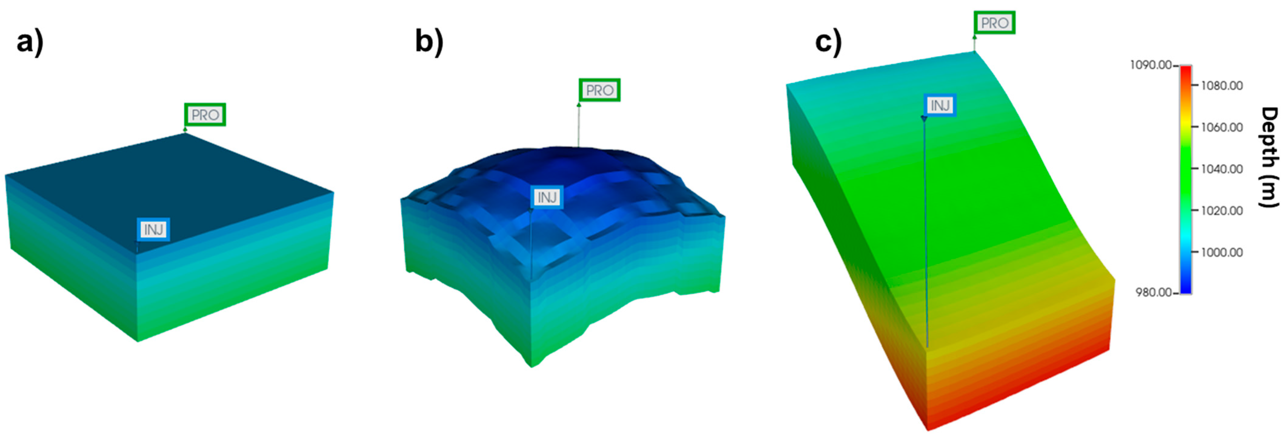
1.3. Reservoir Trap Geometry

Hydrocarbon accumulations within reservoirs must be trapped in place, otherwise petroleum would simply flow through the reservoir. A sealing lithology on top of the reservoir and three dimensional trap are required for an effective petroleum system [25]. Hydrocarbon traps may be either structural, formed by deformation of rocks, or stratigraphic, related to the primary features in the sedimentary structure [50]. Therefore, a trap can be related to the depositional architecture of the rocks or to the structural history of the region, or a combination of the structure and stratigraphy. The two most common types of structural trap are tilted fault blocks, which are observed in the Thistle and Innes fields [26,51], and four-way dip closure anticlines—also known as periclines—that are present within the Blane, Fife, and Forties fields [39,52,53]. The type of trap, whether stratigraphic or structural, can influence the geometry of the oil-bearing unit. Stratigraphic traps are more important in reservoirs with facies-controlled architecture, such as channelised systems and injectites, where sand-rich, porous and permeable reservoir facies are deposited within close proximity to low permeability shales and mudstones; these attributes are present within the Clair, Kraken, and Alba fields [40,41,42].

While there are many publications that focus on accurately defining the complex reactions and kinetic parameters of the oxidation of crude oil during the ISC process, some of these models fail to accurately capture the complexity of the subsurface geology [4,54,55,56,57,58,59]. Reservoir heterogeneity may have an effect on the temperature, velocity, and stability of the fire front as well as the overall three-dimensional structure of the reservoir and its trap. Tilted fault blocks have dipping traps and reservoirs; four-way dip closure pericline folds have complex limbs; structural traps in fluvial systems have complex flow pathways due to the combination of channelised higher permeability volumes and the overlay of structure. The interrelationship of these features means that the geometry of the reservoir will play a significant role in well placement, well spacing and which existing wells could be re-purposed as injectors or producers. If the temperature, velocity, and stability of a fire front could be predicted, this would make decisions on reservoir selection and well placement far easier to make. For the sake of comparability between the models used in this study, the well placements will not change (Figure 1 and Figure 2), however, the performance of the models will be used to discuss where best the wells could be employed as injectors and producers in such systems. Different well arrangements with regard to the heterogeneity distribution or reservoir geometry will not be explicitly modelled in this study.

This study uses three-dimensional numerical models to assess how geological heterogeneity and structure influence the temperature, velocity, stability and potential enthalpy generation of a fire front during the implementation of ISC, to aid in better understanding what types of reservoirs/traps would be best targeted for full field models with detailed bespoke kinetics and fluid parameters. The specific aims of this study are to determine how ISC sector models respond to:

• A four-way dip closure structure, also known as a periclinal fold;
• A tilted fault block, and;
• The added influence of randomly distributed, facies-controlled, and diagenetically controlled heterogeneity within these trap structures.

2. Methodology

This study uses three-dimensional sector models created in the commercial simulation package CMG and run in the simulator STARS (Version 2023.20), which is a three-phase, multicomponent thermal- and steam-additive simulator developed by the Computer Modelling Group Ltd. (CMG), Calgary, AB, Canada [60]. Three-dimensional 29 × 29 × 10 (70 m × 70 m × 25 m) Cartesian grids were constructed with a single injector and producer pairing in a quarter five-spot pattern [4,25]. These models were populated with initial and reservoir conditions (reservoir properties, rock, and fluid thermal properties; well constraints; and injected fluid properties) which do not change between iterations (

Table 1. Initial conditions and reservoir properties used for all simulations.

Reservoir Properties and Initial Conditions	Value
Reservoir property
Initial reservoir temperature (°C)	38
Initial reservoir pressure (kPa)	10,000
Oil saturation	0.5
Water saturation	0.5
Reservoir geometry
Dimensions i, j, k (m)	70 × 70 × 25
Dimensions i, j, k (grid blocks)	29 × 29 × 10
Depth (m)	1000
Rock and fluid thermal properties
Formation compressibility (kPa−1)	1.80 × 10−5
Volumetric heat capacity (J m−3 °C−1)	2.35 × 106
Thermal conductivity phase mixing reservoir rock (J m−3 °C−1)	1.50 × 105
Oil phase heat capacity (J m−3 °C−1)	1.15 × 105
Water phase heat capacity (J m−3 °C−1)	5.45 × 104
Gas phase heat capacity (J m−3 °C−1)	4000
Volumetric heat capacity—overburden (J m−3 °C−1)	2.35 × 106
Volumetric heat capacity—underburden (J m−3 °C−1)	2.35 × 106
Thermal conductivity—overburden (J m−1 day °C−1)	1.50 × 105
Thermal conductivity—underburden (J m−1 day °C−1)	1.50 × 105
Well constraints
Injector well constraints—BHP Max (kPa)	11,000
Injector well constraints—surface gas rate max (m3 day−1)	15,000
Producer well constraints—BHP min (kPa)	9800
Injected fluid
Injected fluid—inert gas (mole fraction)	0.79
Injected fluid—oxygen (mole fraction)	0.21
Injected fluid—temperature (°C)	15
Injected fluid—pressure (kPa)	12,000

), oil parameters (Table 2), and geological parameters (Table 3). Heat loss into the over- and under-burden was included in the models for realistic temperatures using simulator defaults set out by STARS [60,61].

Figure 1. Relative permeability curves used in all simulations: (a) oil–water relative permeability and (b) liquid–gas relative permeability curves with temperature dependence included [62].

Figure 1. Relative permeability curves used in all simulations: (a) oil–water relative permeability and (b) liquid–gas relative permeability curves with temperature dependence included [62].

2.1. Fluid and Reaction Models

For all models, the same volume of air was injected at the same pressure over a simulation of one year. Oil parameters are here based on Mariner oil [63], with pressure, volume, and temperature (PVT) calculations used to model the change in fluid viscosity (Figure 1) [64,65]. Systematic assessment of the effect of varying oil parameters has been undertaken for simpler one-dimensional models in our previous studies therefore was not altered in this study [66]. Gas–liquid “equilibrium” K-values and critical properties for the component “heavy oil” were taken from the STARS manual [60], and the number of carbon atoms has been calculated from the balanced equation (Reactions 1–4). The relative permeability curves (Figure 2) for the fluids are based on typical rocks with water-wet behaviour, as most clastic reservoirs tend to be water-wet [25]; temperature dependence has been included to the relative permeability curves [67] in order to make the output as universal as possible.

Table 2. Fluid model that will be used to compare based on published data from the Mariner field. Pressure–volume–temperature properties of the oils were derived by correlations [64,65].

Component	API Gravity	MW	C Atoms	Pc	Tc	KV1	KV4	KV5	ρ	β	α	μ @ 38 °C
	°API	kg mol−1		kPa	°C	kPa	°C	°C	kg m−3	kPa−1	°C−1	Cp
Heavy oil	14	0.355	22	853.1	508.8	1,726,140	−5214.3	−114.5	928.4	9.08 × 10−7	2.96 × 10−3	2118.8
Light oil	-	0.027	-	2710.0	318.5	4,890,000	−4655.9	−273.2	742.0	1.00 × 10−6	9.00 × 10−4	40.1
H2O	-	0.018	-	-	-	-	-	-	994.9	4.43 × 10−7	3.79 × 10−4	0.8
CO2	-	0.028	-	7376.4	31.1	5,323,400	−2002.1	−273.2	500.0	5.98 × 10−6	2.96 × 10−3	0.1
O2	-	0.032	-	5046.0	−118.6	5,323,400	-	-	-	-	-	-
NCG	-	0.028	-	3394.4	−147.0	906,661	−705.2	−273.2	318.0	6.00 × 10−6	3.00 × 10−5	1.7
Coke	-	0.012	-	-	-	-	-	-	917.0	-	-	-

Table 2. Fluid model that will be used to compare based on published data from the Mariner field. Pressure–volume–temperature properties of the oils were derived by correlations [64,65].

Component	API Gravity	MW	C Atoms	Pc	Tc	KV1	KV4	KV5	ρ	β	α	μ @ 38 °C
	°API	kg mol−1		kPa	°C	kPa	°C	°C	kg m−3	kPa−1	°C−1	Cp
Heavy oil	14	0.355	22	853.1	508.8	1,726,140	−5214.3	−114.5	928.4	9.08 × 10−7	2.96 × 10−3	2118.8
Light oil	-	0.027	-	2710.0	318.5	4,890,000	−4655.9	−273.2	742.0	1.00 × 10−6	9.00 × 10−4	40.1
H2O	-	0.018	-	-	-	-	-	-	994.9	4.43 × 10−7	3.79 × 10−4	0.8
CO2	-	0.028	-	7376.4	31.1	5,323,400	−2002.1	−273.2	500.0	5.98 × 10−6	2.96 × 10−3	0.1
O2	-	0.032	-	5046.0	−118.6	5,323,400	-	-	-	-	-	-
NCG	-	0.028	-	3394.4	−147.0	906,661	−705.2	−273.2	318.0	6.00 × 10−6	3.00 × 10−5	1.7
Coke	-	0.012	-	-	-	-	-	-	917.0	-	-	-

Table 3. Geo-models that were used to test different heterogeneity patterns and reservoir geometries on the propagation of the fire front, with the Dykstra–Parsons permeability coefficient.

Geo-Model	Sub-Model	Geometry	Type	Porosity (%)	Permeability (mD)	kv/kh	V
1	A	Cube	Uniform	20	700	0.1	0
	B	Cube	Random	20	700	0.1	0.66
	C	Cube	Facies	5 (20 Channel)	7 (700)	0.1	0.05
	D	Cube	Layered	5 (20)	8 (700)	0.1	0.95
2	A	Pericline	Uniform	20	700	0.1	0
	B	Pericline	Random	20	700	0.1	0.66
	C	Pericline	Facies	5 (20 Channel)	7 (700)	0.1	0.05
	D	Pericline	Layered	5 (20)	8 (700)	0.1	0.95
3	A	Tilted block	Uniform	20	700	0.1	0
	B	Tilted block	Random	20	700	0.1	0.66
	C	Tilted block	Facies	5 (20 Channel)	7 (700)	0.1	0.05
	D	Tilted block	Layered	5 (20)	8 (700)	0.1	0.95

Table 3. Geo-models that were used to test different heterogeneity patterns and reservoir geometries on the propagation of the fire front, with the Dykstra–Parsons permeability coefficient.

Geo-Model	Sub-Model	Geometry	Type	Porosity (%)	Permeability (mD)	kv/kh	V
1	A	Cube	Uniform	20	700	0.1	0
	B	Cube	Random	20	700	0.1	0.66
	C	Cube	Facies	5 (20 Channel)	7 (700)	0.1	0.05
	D	Cube	Layered	5 (20)	8 (700)	0.1	0.95
2	A	Pericline	Uniform	20	700	0.1	0
	B	Pericline	Random	20	700	0.1	0.66
	C	Pericline	Facies	5 (20 Channel)	7 (700)	0.1	0.05
	D	Pericline	Layered	5 (20)	8 (700)	0.1	0.95
3	A	Tilted block	Uniform	20	700	0.1	0
	B	Tilted block	Random	20	700	0.1	0.66
	C	Tilted block	Facies	5 (20 Channel)	7 (700)	0.1	0.05
	D	Tilted block	Layered	5 (20)	8 (700)	0.1	0.95

Figure 2. Viscosity vs. temperature graphs to illustrate how the initial oil viscosity decreases with increasing temperature [64,65].

Figure 2. Viscosity vs. temperature graphs to illustrate how the initial oil viscosity decreases with increasing temperature [64,65].

As the main focus of this study is the role of reservoir geology and petrophysics on the efficacy of ISC, a simple reaction model was adopted here, based on Crookston’s model [68]. The model is the most commonly employed reaction scheme in ISC simulations [69]. This simple scheme is suitable to assess the geological controls on ISC because it has been reported that relatively simple reaction models with fewer components perform well when compared to more complex schemes with large numbers of components [70].

There are seven components in this reaction scheme: oxygen, non-condensable gas (NCG), carbon dioxide, water, coke, a heavy hydrocarbon pseudo-component, and a light hydrocarbon pseudo-component; properties of each component are given in Table 2, and kinetics for the four reactions listed below are given in

Table 4. Reaction stoichiometry and reaction kinetics for the different oil models.

Reaction	Ea1 (J mol−1)	A (day−1 kPa−1)	H (J mol−1)
1	2.10 × 105	3.34 × 1016	0
2	1.32 × 105	5.69 × 1012	2.01 × 107
3	5.34 × 104	4.86 × 1011	2.16 × 106
4	3.41 × 104	2.49 × 105	2.00 × 105

.

The four reactions are:

$$1heavyoil\to 2.83lightoil+23.37coke$$

(R1)

$$1heavyoil+29.63O_2\to 18.10C{O}_2+22.57H_{2}O+3.62NCG$$

(R2)

$$1lightoil+2.25O_2\to 1.19C{O}_2+2.22H_{2}O+2.24NCG$$

(R3)

$$1coke+1O_2\to 0.73C{O}_2+0.44H_{2}O+0.15NCG$$

(R4)

2.2. Geological Models

The geological models (3D Cartesian grids populated with petrophysical properties) were constructed in CMG Builder [60]. There are three structures: a cube, a periclinal four-way dip closure, and a tilted fault block (Figure 3). Each structure has been paired to one of four heterogeneity patterns: a homogeneous petrophysical properties (the control model), randomly distributed petrophysical properties, depositional facies controlled petrophysical properties, and diagenetically controlled horizontally layered petrophysical properties (Figure 4). The three structures and four petrophysical heterogeneity patterns result in a total of 12 models. Each trapping structure is assigned a number, 1 to 3, and each heterogeneity pattern is a assigned a letter, A to D (Table 3); for example, a periclinal fold with layered heterogeneity will be referred to as Model 2-D, a cube with no heterogeneity will be 1-A, etc.

Randomly distributed porosity models represent normally distributed grid block scale heterogeneity (2.4 × 2.4 m) with spatially distributed porosity variations. Although the control on porosity is not defined in the model, it could be derived from either grain size distribution and sorting during deposition or by diagenetic processes, such as cementation after deposition. Randomly distributed porosity models have a mean porosity of 20% with a standard deviation of 6%. This random pattern was created by the use of 400 points, or “wells”, with randomly assigned X, Y, and Z coordinates and then given a porosity value based around the mean and standard deviation; this distribution was then interpolated through the use of kriging with a spherical variogram.

Facies-controlled heterogeneities have been based on a macroscopic flow unit—in this case, a 24 m wide and 12 m deep meandering channel, with 20% porosity within the channel and 5% porosity in the surrounding sediments.

For the homogeneous control model, the permeability was fixed at 700 mD horizontal permeability. For all other models, the permeability was based on a simplified Kozeny–Carman equation [71,72], which derives permeability from spatially variable porosity and grain size:

$$\mathit{k}={\displaystyle \frac{{\mathit{\phi }}^3·{\mathit{D}}^2}{180·{\left(1-\mathit{\phi }\right)}^2}}$$

(1)

where k is permeability, φ is porosity, and D is grain diameter. For these models, a constant 200 μm grain diameter has been employed, as this is a common grain size in clastic sandstone oil reservoirs [25,27,50]. Permeability heterogeneity has been quantified by the Dykstra–Parsons permeability coefficient, (Table 3); the closer the coefficient is to 1, the more heterogeneous the system is [73]. All models here have a vertical to lateral permeability (k_v/k_h) ratio of 0.1 within the grid block.

As the main focus of this study is to assess the feasibility of reactivating abandoned, depleted oil fields to generate heat as an enhanced geothermal system, an initial (residual) oil saturation of 0.5 was used to represent a depleted reservoir of which had an initial oil saturation of 0.8 and a recovery factor of 35% [9].

2.3. Key Aspects of Model Outputs

To assess the temperature, velocity, and propagation stability of the fire front, the six hottest points of the fire front have been extracted for each vertical layer and an average taken for the temperature, velocity, and propagation angle with respect to the producer taken for each of the points. Each simulation was run initially for one year then analysed to differentiate the effects of the geometry and heterogeneity on the peak temperature, velocity, and stability of the fire front. The same models were then run for 5 years to measure the peak enthalpy rate and arrival time at the producer well to ascertain the viability of each scenario as an enhanced geothermal system.

3. Results

3.1. Petrophysically Homogeneous Models (Model A)

3.1.1. Cube Geometry (Model 1-A)

Model 1-A (Figure 5a) has a symmetrically shaped fire front moving along behind a bank of oil, which is visible by the increase in oil saturation ahead of the fire front. The fire front is migrating evenly across the grid with a point towards the production well; the fire front is moving in a wedge shape with more movement towards the top of the grid than the bottom, elongating the top relatively more than the bottom (Figure 5a). The temperature distribution (Figure 6a) reveals an average temperature of 362 °C at the top of the reservoir, increasing to a peak of 715 °C at Layer 8 and then decreasing to 197 °C towards the base of the reservoir. The velocity of the fire front is greatest, 0.12 m·day⁻¹, at the top of the reservoir (Figure 6b), with a decrease at Layer 2 to 0.07 m·day⁻¹, followed by a steadier decrease at Layer 10, where the lowest velocity of 0.02 m·day⁻¹ is observed. The stability of the fire front is steady throughout the grid (Figure 6c), with no deviation away from the direct path between injector and producer.

3.1.2. Four-Way Dip Closure (Model 2-A)

Model 2-A has a wedge-shaped fire front propagating evenly across the grid (Figure 5b) with concentration of the oil (high oil saturation) away from the base of the reservoir; there are slight distortions in the shape of the fire front at the top layer of the grid. The average temperature across the fire front is 377 °C at the top of the grid (Figure 6a) and increases to a peak of 921 °C at Layer 4. There is a sudden sharp decrease down to 230 °C at Layer 6 and then a steady decline to 190 °C at Layer 10. The velocity of the fire front is highest at the top, moving at an average of 0.07 m·day⁻¹ and decreasing after Layer 2 to 0.02 m·day⁻¹ at Layer 5, followed by a steady drop to 0.01 m·day⁻¹ to Layer 10 (Figure 6b). The propagation of the fire front has a subtle deviation to the left of the grid at the top layer, although below this top layer there is no significant deviation away from the direct path (Figure 6c).

3.1.3. Tilted Fault Block (Model 3-A)

The fire front moves up-dip and straight up the side of the fault block, towards the top-left corner, with little residual oil left at the bottom of the structure (Figure 5c). The temperature at the top layer is 483 °C, which increases to a peak of 859 °C in Layer 2; this is then followed by a sharp drop to 387 °C in Layer 3 and a steady decline thereafter to Layer 10 (Figure 6a), with a minimum temperature of 83 °C. The velocity of the fire front is highest at the top layer, with a value of 0.09 m·day⁻¹, decreasing throughout the simulation to the lowest value observed of 0.01 m·day⁻¹ (Figure 6b). The fire front propagates sharply to the left of the grid throughout the simulation through most of the layers; the lowermost layers, 9 and 10, propagate more towards the middle (Figure 6c).

3.2. Randomly Distributed Petrophysical Heterogeneity (Model B)

3.2.1. Cube Geometry (Model 1-B)

The random porosity and permeability pattern in Model 1-B has resulted in a distorted fire front; the greatest amount of displacement of oil is towards the top of the grid, with less toward the bottom (Figure 7a). Elevated oil saturation develops around the bottom of the injection well (Figure 7a). The average temperature of the fire front starts at 362 °C, at the top of the grid, with a slight increase to the highest observed temperature of 449 °C at Layer 4, followed by an irregular decrease to 254 °C, towards Layer 10 (Figure 8a). The highest velocity of the fire front is at the top, with Layer 1 having a value of 0.14 m·day⁻¹ (Figure 8b). There is an irregular decrease in velocity towards Layer 6, followed by a sharp drop to 0.02 m·day⁻¹ in Layer 7, where it remains low all the way to the base of the reservoir (Figure 8b). The fire front at the top of the reservoir has a sharp deviation to the left of the grid, with more stable propagation below Layer 6 and to the base of the reservoir (Figure 8c).

3.2.2. Four-Way Dip Closure (Model 2-B)

Model 2-B has a distorted fire front, with highest oil saturation towards the top of the grid, with little residual oil around the injector well (Figure 7b). The average fire front temperature is 379 °C at the top of the grid, with an irregular increase to the highest observed value, 563 °C, in Layer 6 and a sharp decrease to 225 °C at the base of the reservoir. The velocity of the fire front at the top of the grid is 0.07 m·day⁻¹; there is a decrease in velocity down to Layer 6 at 0.02 m·day⁻¹, where it remains low at the base of the reservoir (Figure 8b). The stability of the fire front reveals some movement to both the right and left of the direct path; overall the entire fire front tends to propagate along the direct path toward the production well (Figure 8c).

3.2.3. Tilted Fault Block (Model 3-B)

The tilted fault block model, with randomly distributed porosity and permeability heterogeneity, has a strong preference for the fire front to travel up-dip, with the entire top of the left side of the model swept, there are two smaller fire fronts moving towards the middle of the structure and migrating in the direction of the production well (Figure 7c). The average fire front temperature for Layer 1 is 418 °C, the peak temperature is observed in Layer 2 at 800 °C, followed by a sharp decrease down to Layer 3 where the temperature is 386 °C and a steady decrease down to Layer 10, where the lowest temperature (91 °C) occurs (Figure 8b). The velocity of the fire front is highest in Layer 3 (0.17 m·day⁻¹); velocity decreases upwards toward Layers 1 and 2 as well as downwards toward Layer 4. Velocity decreases steadily below Layer 4 to the lowest value of 0.01 m·day⁻¹ in Layer 10 (Figure 8b). The stability of the fire front is somewhat irregular but mostly tends towards the left of the structure (i.e., close to 0°); there are some deflections to the right, representing the smaller arms of the fire front at the top of the reservoir. Fire front propagation is more stable in the lower part of the reservoir than in the upper layers (Figure 8c).

3.3. Facies Controlled Petrophysical Heterogeneity (Model C)

3.3.1. Cube Geometry (Model 1-C)

Model 1-C reveals the movement of residual oil into the channel structure of the facies model to the right of the injection well; there is little movement of oil in the immediate area around the well, and the fire front does not develop outside of the depositional channel structure (Figure 9a). The temperature distribution graph illustrates that the highest temperature, 342 °C, was observed in Layer 1 at the top of the reservoir; the temperature then steadily decreases downwards to Layers 6 to 10 which record maximum temperatures of only 75 °C (Figure 10a). The velocity profile shows the highest values (0.05 m·day⁻¹) occur at Layer 1, followed by a stepped decrease down to a low of 0.01 m·day⁻¹ in the lowest layer (Figure 10b). There is a strong deviation to the right of the grid in the top seven layers as the fire front follows the path of the channel rather than the shortest path between injector and producer wells; at deeper levels, there is no deviation, as the fire front is effectively absent in Layers 7 to 10 (Figure 10c).

3.3.2. Four-Way Dip Closure (Model 2-C)

The periclinal fold model with a channel (i.e., the facies model) displays the initiation of a small fire front beginning to develop (Figure 9b). High oil saturation develops near to the top of the reservoir close to the injection well with a subtle movement towards the depositional channel structure (Figure 9b). The highest average temperatures (305 °C) occur in Layer 1; this decreases sharply to 155 °C in Layer 2 and then falls away to ambient conditions in Layer 6 and deeper (Figure 10a). The average velocity of the fire front is at its maximum in Layer 1 (0.03 m·day⁻¹) and decreases in Layer 2 and again in Layer 3, where it stays around 0.01 m·day⁻¹ in reservoir Layers 4 to 10 (Figure 10b). There are subtle deviations of the fire front to the right side of the grid towards the location of the channel as deep as Layer 5, but none occur in deeper layers, as the fire front is absent in this part of the structure (Figure 10c).

3.3.3. Tilted Fault Block (Model 3-C)

Model 3-C has a subtle increase in oil saturation around the injector well; however, there is no indication of the development of a well-defined fire front in this modelled system (Figure 9c). The temperature profile is effectively flat, as there is an average peak temperature of 67 °C at Layer 1 and then a trivial increase to 72 °C at Layer 5 then decreasing again to 65 °C all the way to the base of the reservoir (Figure 10a). Given the weak development of a fire front, there are negligible velocities and deviations from the 45° default angle (Figure 10b,c).

3.4. Diagenetically Controlled Petrophysically Layered Reservoir (Model D)

3.4.1. Cube Geometry (Model 1-D)

Model 1-D illustrates the fire front propagating through the reservoir evenly in a pointed shape; however, the oil saturation varies by layer, with strongly elevated oil saturations in the higher porosity and permeability layers but insignificant changes in the other layers (Figure 11a). Despite this, the fire front is well developed in the model (Figure 11a). The temperature profiles have a sawtooth pattern, with higher temperatures observed within the higher porosity and permeability layers—for example, Layers 1 and 3, where the temperatures are 352 and 400 °C (Figure 12a). Conversely, the lower-porosity and permeability Layers 2 and 4 achieve relatively low temperatures of 254 and 276 °C. The velocity in Layer 1 is 0.11 m·day⁻¹, this decreases in a sawtooth pattern to a low of 0.05 m·day⁻¹ with the higher porosity and permeability layers having the higher velocity values (Figure 12b). The stability of the fire front is not affected by the layering in this model, there is a simple, unperturbed propagation of the fire front from the injector to the producer well (Figure 12c).

3.4.2. Four-Way Dip Closure (Model 2-D)

Model 2-D shows a uniform propagation of the fire front across the reservoir, with higher oil saturation and greater oil movement through the layers with higher porosity and permeability (Figure 11b). The temperature profile mirrors that of the cube model, with the higher porosity and permeability layers, such as 1 and 3, having high temperatures (363 and 447 °C, respectively) and the lower-porosity and permeability layers, such as 2 and 4, having lower temperatures, (315 and 353 °C, respectively). The average velocity of the fire front at Layer 1 is 0.03 m·day⁻¹. This increases up to Layer 3 at 0.07 m·day⁻¹. After this, there is an alternating pattern of higher velocity in the higher-porosity and permeability layers—for example, 0.07 m·day⁻¹ in Layer 3 and lower velocity in the lower-porosity and permeability layers, such as the 0.05 m·day⁻¹ seen in Layer 4 (Figure 12b). The stability of the fire front has not been affected by the interlayering of high- and low-porosity and permeability layers (Figure 12c).

3.4.3. Tilted Fault Block (Model 3-D)

The fire front has preferentially migrated up-dip and to the left of the grid, with oil saturation increasing in layers of higher porosity and permeability (Figure 11c). The temperature distribution by layer has higher temperatures in the higher porosity and permeability layers, such as 413 and 468 °C in Layers 1 and 3, respectively, and 335 and 375 °C in Layers 2 and 4, respectively. There is a steady decrease below Layer 8 to a minimum temperature to 263 °C (Figure 12a). The velocity profile has an alternating pattern down the layers, with lower velocity seen within higher-porosity and permeability layers; for example, Layers 1 and 3 have velocities of 0.08 and 0.07 m·day⁻¹, respectively and Layers 2 and 4 both have velocities of 0.09 m·day⁻¹ (Figure 12c). The propagation angle of Model 3-D has a strong deviation to the left of the line between the injector and producer well for the entire stratigraphic succession (Figure 12c).

3.5. Effect on Enthalpy at the Production Well

The enthalpy rate over 5 years differs for each model depending on the geometry and heterogeneity present (Figure 13). Models 2-A, 3-A, and 3-B failed to run for the 5-year duration or did not produce any significant enthalpy, so they have not been included in Figure 13. Models 1-C, 2-C, and 3-C, all models with a depositional channel, produced very low enthalpy rates throughout the simulation duration and peaked only at the end of the simulation, with peak rates of 2, 0.7, and 1.1 MJ·day⁻¹. Models without geometry and without sharply defined stratigraphic channels—1-A, 1-B, and 1-D—are among the earliest to begin enthalpy production and earliest to peak, with peak rates seen at year 4 for 1-A at 7200 MJ·day⁻¹ and year 2 for B and D at 10,500 and 12,400 MJ·day⁻¹, respectively. The remaining models are 3-D, producing 6900 MJ·day⁻¹; 2-B, producing 11,800 MJ·day⁻¹; and 2-D, producing 9600 MJ·day-1 (Figure 13).

4. Comparison of Models and Discussion

4.1. The Effect of Trap Geometry

To assess the effect of the geometry of the reservoir on the ISC process, for each different heterogeneity type, the periclinal fold and the tilted fault block have been compared to the basic cube model as a base case, and the differences in temperature, velocity, and propagation stability have been compared.

4.1.1. Trap Geometry and Temperature

Homogeneous Reservoir

The distribution of average temperature across the layers of the reservoir is different depending on the geometry of the reservoir. When comparing the cube to the periclinal fold for homogenous models 1-A to 2-A (Figure 14a), there is a similar temperature at the top layer, however, moving downwards the temperature is greater in the periclinal fold by up to 493 °C compared with the cube model. Below Layer 6, the temperature is lower in the pericline structure than the cube by up to 475 °C. At Layer 10, the base of the grid, the temperature is similar in both. The buoyancy of the heated oil appears to be greater in the pericline than the cube, the cracking of the oil and the decreases in density that follows increases the buoyancy, the natural movement of the lighter oil is towards the culmination of the structure in the pericline as a result [25] (Figure 5b), this is not observed in the cube as there is no structure present to collect the oil. This means that the fuel deposition is likely to preferentially occur higher up the periclinal structure than it does in the cube model, where there is a relative enrichment of oil saturation around the base of the fire front (Figure 5a). The tilted fault block also has a similar temperature in Layer 1 to the cube model, then in Layer 2, it is 423 °C hotter. Layer 3 and deeper have temperatures that are up to 581 °C lower; Layer 10 has similar temperatures in the tilted fault block and the base case (Figure 14a).

Randomly Distributed Heterogeneity

With the addition of randomly distributed heterogeneity in model-2 (Figure 14b) the periclinal fold has higher temperatures than the cube for most of the layers of the model. Model-1-B (Figure 8a) has a much more even distribution of temperature down the layers of the grid than model-1-A, which has a large spike in temperature at Layer 8 (Figure 6a). The tilted fault block has an almost inverse effect on the temperature than the pericline when compared with the cube, with hotter temperatures at the top and cooler temperatures than the cube at the bottom of the structure (Figure 14b).

Facies Controlled Heterogeneity

The channelled models have, in both cases, much lower temperatures than in the base case (Figure 14c), especially in the tilted fault block, where the temperature does not exceed 77 °C (Figure 10b) and therefore does not commence coke (fuel) deposition or begin HTO reactions. In both cases, the fire front is likely to extinguish before it can become self-propagating [74].

Layered Reservoir

For the layered models (Figure 14d), the temperature is always greater in the pericline and tilted fault block than the cube, with the exception of Layer 9 in the tilted fault block, which is 108 °C lower than the cube (Figure 14d). The fire front remains relatively well connected vertically in all layered models despite the differences in porosity and permeability in the alternating layers (Figure 11). This is in comparison to the homogenous models, in which the fire front is moving at a much higher velocity at the top than the bottom, creating a wedge-shaped fire front not observed in the layered models. Although the lower-porosity and permeability layers are not fully swept in any of the layered models (Figure 11), the vertical conduction of temperature through the layers is enough for the fire front to stay in vertical communication allowing the front to remain thermally coupled across the layers. Greater thickness of such interbedded lower quality reservoirs may cause problems with the vertical temperature communication of the fire front and cause the fire front to become thermally uncoupled and split [75,76]. The layering of high and low porosity and permeability makes it more difficult for the oil to move vertically than in the cube, inhibiting the upwards flow of injected air and the movement of oil below the fire front, as occurs in Model 1-A.

4.1.2. Trap Geometry and Velocity

Homogeneous Reservoir

Comparing the pericline to the cube structure for the homogenous model, the velocity is 0.05 m·day⁻¹ lower in Layer 1 in the pericline (Figure 15a). Deeper in the grid, the velocity is less different, although always lower in the pericline than the cube. The pattern is similar in the tilted fault block (Figure 15a), with a lower velocity in the top layer and a more similar velocity below, although Layers 4 and 5 in the tilted fault block have marginally higher velocity than what is observed in the cube. The effect of the geometry on the velocity of the front is most pronounced in the very top layer in both the pericline and the tilted fault block. The observed difference in velocity in the pericline and fault block the homogeneous model and the heterogeneous model, lower at the top, are a result of the movement of oil up the structure against gravity, which is not observed within the cube model as there is no upwards movement.

Randomly Distributed Heterogeneity

For randomly distributed heterogeneity models (Figure 15b), the velocity in the pericline is lower in the upper seven layers and more similar in the lower three to the cube model. The tilted fault block follows a similar pattern with the exception of Layer 3, where it is 0.1 m·day⁻¹ faster than the cube model, likely caused by the preferential migration of the front up-dip in the periclinal fold, where it will encounter a different porosity and permeability arrangement to the cube model that facilitates a different velocity to that in the same pattern in the cube.

Facies Controlled Heterogeneity

With the channelled models, the velocity is lower in the upper five layers in both the pericline model and the tilted fault block than the cube model (Figure 15c). The velocity in the upper layers of the pericline and tilted fault block models with channels is low for the pericline and tilted fault block (Figure 10b) because the fire front never reaches the channel in these models (Figure 9b,c).

Layered Reservoir

When comparing the pericline model back to the cube model with layered heterogeneity, the pericline always has a lower temperature than the cube. This is particularly evident in the top layer of the reservoir (Figure 15d). The tilted fault block shows in the higher porosity and permeability layers—Layers 1, 3, 5, etc.—that the temperature is lower than that of the cube. The temperature in the lower-porosity and permeability layers—2, 4, 6, etc.—is higher than that of the cube models (Figure 15d).

4.1.3. Trap Geometry and Fire Front Propagation Stability

Homogeneous

The propagation stability is affected by the geometry of the grid in the absence of any heterogeneity (Figure 16). In the homogenous models (Figure 16a), the pericline has little difference in stability to the cube model other than a few deviations in the upper layers. The tilted fault block has a large deviation of the fire front to the left of the grid from the injector well and has a strong preference to travel directly up-dip and, in this case, to the left-hand side of the grid as opposed to directly towards the producer well as in the cube and pericline.

Randomly Distributed Heterogeneity

Randomly distributed heterogeneity leads to subtle differences in fire front propagation in the tilted fault block and the pericline, with the top layers of the pericline having some difference in stability compared to the cube but, from Layer 5 down, they have a similar propagation pattern to the cube (Figure 16b). The tilted fault block has a similar pattern to the pericline in the top four layers, followed by a sharp deviation to the left, with a preference to migrate directly up-dip and to the top-left of the grid (Figure 16b).

Facies Controlled Heterogeneity

The channelled models lead to considerable differences in fire front propagation stability, as the cube model is the only model in which the fire front reaches the channel (Figure 9). The fire front has been forced to follow the path of the channel and, consequently, has been deflected to the right side of the grid (Figure 10c). In contrast, in the pericline and tilted fault block models, there is no significant formation of a fire front (Figure 9b,c). The presence of a channel system and subsequent juxtaposition of good- and poor-quality reservoirs creates difficulty in forming the fire front when the injection well is located in the poor-quality reservoir.

Layered Model

The layered model has a similar fire front propagation pattern as the homogeneous models, with the pericline model following a similar path to the cube model and the tilted fault block in preferentially migrating up-dip to the top-left of the grid. This movement pattern is sustained all the way to Layer 10 in the layered model (Figure 16c).

Increases in temperature and the subsequent cracking of the oil have reduced the density of the oil and therefore the buoyancy. This causes a preferential migration of the oil up-dip towards the apex of the trapping structure where it concentrates [25] and, in this case, to the left as a result of the positions of the wells. This outcome highlights the importance of understanding the relationship of the geological structure and the well-positioning to ensure the wells are used to maximum efficiency. This is important in the absence of heterogeneity and even more important in situations in which the heterogeneity also affect the relative movement of the fire front, where the structure appears to have a greater influence.

4.1.4. Trap Geometry and Enthalpy

The cube models are the first to begin producing enthalpy, producing peaks at the 2-year mark, earlier than any pericline or tilted fault block models (Figure 13). In the cases with reservoir geometry there is no clear control exerted on the timing of the enthalpy or the amount of enthalpy generated due to changing the geometry of the reservoir as all different geometries produce the same order of magnitude of enthalpy (Figure 13).

4.2. The Effect of Heterogeneity

Each of the heterogeneities has been compared to the homogeneous model for the same trap type. For example, the difference in temperature has been plotted from the random heterogeneity model to the homogenous model for the cube model, Model 1-B to 1-A, etc.

4.2.1. Type of Heterogeneity and Temperature

Cube

Comparing the base case homogenous model (1A) to the randomly distributed heterogeneous model (1B), the temperature profile is similar for the top six layers (Figure 17a); it is then considerably lower for Layer 8 (448 °C) for the randomly distributed heterogeneous model than the homogeneous model. Homogeneous cube Model 1-A has a high average peak temperature in Layer 8 (Figure 6a), the wedge-shaped fire front with greater movement at the top and less and the bottom appears to force a relative concentration of oil saturation below the fire front, leading to greater fuel deposition and higher temperatures at this layer (Figure 5a). The heavier fraction of oil tends to sink, this is what then goes on to form coke (fuel), leading to higher temperatures. The concentration of oil below the front does not appear to happen once heterogeneity is introduced (Figure 7a); this is due to the lower initial oil volumes introduced by the heterogeneity.

The same difference in temperature at Layer 8 is observed in both the channelled model and the layered model also, where they have considerably lower temperatures at this point than observed in the homogenous model (Figure 17a). The temperature is lower for every layer in the channelled model than it is in the homogeneous model. This temperature difference is due to the lower porosity, and therefore lower oil saturation and lower coke (fuel) deposition, in the rock surrounding around the channel, i.e., poor-quality reservoir. The resultant temperature differences observed has important implications for the location of the wells, for exploitation of higher temperatures the wells would be better placed within higher porosity flow units and perforated only within them.

There is little difference between the temperatures in the higher porosity layers of the layered model and the homogeneous model for the top five layers (Figure 17a). The lower five layers of the layered model have considerably lower temperatures, in particular Layer 8. Other than this, the fire front stays in good vertical communication through the layers in this model.

Periclinal Fold

For the periclinal fold models, the top five layers of the three heterogenous models all display lower temperatures than the homogenous model (Figure 17b). For the lower five layers, the randomly distributed and layered models have higher temperatures than the homogenous model. The channelled model always has lower temperature than the homogenous model, although the effect is less pronounced in the lower layers than in the upper layers.

Tilted Fault Block

The randomly distributed heterogeneity model has little variation in the temperature of all layers when compared to the homogeneous model (Figure 17c). Both the channelled and the layered models have lower temperatures in Layer 1 and much lower temperatures in Layer 2; after this, the channelled model has a lower temperature than the randomly distributed heterogeneity model in the lower layers. The layered model has a higher temperature in the lower layers than that of the homogeneous model, which is a result of the more vertically consistent shape of the oil bank and fire front in this model (Figure 11) compared to the wedge-shaped fire front seen in homogeneous models, in which the top of the front moves much faster than the bottom (Figure 5). With the lack of a fire front forming in the lower areas of the channelled model, the injected oxygen will not be utilised in reactions and could potentially migrate around or away from the fire front, leading to the extinction of the front or to potentially dangerous oxygen production [4].

4.2.2. Type of Heterogeneity and Velocity

Cube

For the cube model, the velocity is slightly higher in the randomly distributed model for the upper six layers than the homogeneous model, but it is slightly lower in Layers 7 to 11. This pattern is due to the random nature of differences in the porosity and permeability of the random heterogeneous model compared to the homogeneous model (Figure 18a). The channelled model has a lower velocity than the homogenous model for all layers, with a greater decrease in the upper layers than the lower layers. The velocity of Layer 1 for the layered model is slightly lower than that in the homogeneous model. However, for all other layers, the velocity is always higher in the layered reservoir than the homogeneous (Figure 18a) and is far more vertically consistent in shape.

Periclinal Fold

The pericline fold model with random heterogeneity has a similar velocity to the homogenous model for the top three layers, with a slightly higher velocity in Layers 4 and 5 then a slight decrease in most lower layers, although Layer 10 has a near-identical velocity between the homogeneous and random heterogeneity model (Figure 18b). The channelled model has a much lower velocity than the homogeneous model until Layer 9, where the velocity is near identical to the cube and the pericline. This is because there is almost no movement of the fire front in any models with a channel below Layer 5 (Figure 10b). With the exception of the cube model there is little or no fire front development in the channelled model in any case (Figure 9). Similarly to the cube model, other than the top 2 layers, the layered reservoir shows greater velocity than the homogeneous one (Figure 18b) and is once again more vertically consistent.

Tilted Fault Block

Despite a spike in the velocity in the randomly distributed model at Layer 3 there is little difference in the velocities seen between this and the homogeneous model in the tilted fault block geometry (Figure 18c). The velocity is always lower in the channelled model until the bottom 2 layers, where there is almost no movement of the fire front in the homogeneous or randomly distributed models either. The layered model has a higher velocity for the duration of the simulation than the homogeneous model (Figure 18c). The layered model has a pattern of higher velocity followed by lower velocity, with higher velocities in the higher porosity layers and lower velocities in the lower-porosity layers (Figure 12b) for the cube and the pericline, and the opposite for the tilted fault block. One-dimensional modelling revealed that lower-porosity models and higher-permeability models display higher velocities [66], it is apparent in the cube and the pericline that the permeability is controlling the velocity, and in the tilted fault block, the porosity appears to have a greater affect.

4.2.3. Type of Heterogeneity and Fire Front Propagation Stability

Cube

For the cube models, the propagation stability is controlled entirely by the heterogeneity, with the propagation of the homogenous model being entirely stable and along the line between injector and producer (Figure 6c). The randomly-distributed model has a strong deviation to the left of the grid, likely following a path of easier flow (higher permeability) and greater oil volume (higher porosity) (Figure 19a), i.e., better reservoir quality [25]. The fire front has migrated towards the channel in the cube model—a relative movement to the right in this case (Figure 19a).

Periclinal Fold

The introduction of the periclinal fold geometry creates complex patterns of propagation stability throughout the grid (Figure 19b). There is a slight preference of movement to the right of the grid in Layer 1 in all models, followed by an irregular difference below, although there is no clear pattern to this and there is some relative movement to the left and to the right. The overall movement direction is the direct path between injector and producer, with a preference for the fire front to move towards the culmination at the centre of the structure (Figure 1b) and is effectively uninfluenced by the heterogeneity patterns.

Tilted Fault Block

With the exception of the channelled model, where there is no fire front initiated (Figure 9c), the movement of the fire front in the tilted fault block model is always preferentially up-dip, to the top-left of the grid (Figure 5c, Figure 7c and Figure 11c), and appears largely unperturbed by the changes in heterogeneities (Figure 19c). The randomly distributed model has some movement towards the production well (Figure 7c) likely as the result of an easier flow pathway present and some channelling of the fire front and may cause the fire front to split and become uncoupled if the differences in porosity or permeability are large enough.

4.2.4. Types of Heterogeneity and Enthalpy

In all cases, the channel model produces very low enthalpy rates over 5 years (Figure 13). When comparing only the cube models, the layered reservoir produces the greatest enthalpy rates. The same is true for the tilted fault block model with the layered reservoir (Figure 13). The periclinal fold model shows the highest enthalpy rates in the randomly distributed heterogeneity model and then the layered model (Figure 13).

4.3. Overall Controls

Although there are differences in the temperature in the various layers due to the geometry of the reservoir, the overall effect of the geometry when taking all the differences into account and comparing them to the basic cube model appears to be negligible, i.e., the median temperature difference is 0 °C (Figure 20a). The control on temperature is different in the different geometry models, with the exception of the channelled models, the general trend shows that the pericline and the fault block display hotter temperatures in the upper layers, and cooler temperatures in the lower layers than the base case cube model (Figure 14).

The median effect of adding heterogeneity into the models (using all data from random, channelled, and layered simulations) is to reduce the overall temperature compared to the homogeneous case (Figure 20a). This is most apparent in the channelled models that have negligible fire front development. Notable exceptions to the decrease in temperature are the layered versions of both the tilted fault block and the pericline structures, where they display higher temperatures than the cube (Figure 14d).

The heterogeneity of the reservoir has an overall effect of slightly decreasing the velocity (Figure 20b), although there are range of effects, most notably in the tilted fault block. Overall, adding complexity to the geometry of the reservoir (pericline and tilt block versus a cube) also acts to reduce the velocity of the fire front in most cases, again with the exception of the randomly distributed pericline model. The introduction of layered reservoirs in all cases acts create a more consistent vertical velocity profile than is observed within a homogeneous model (Figure 12b).

The overall effect of heterogeneity on the propagation stability is to move the fire front slightly to the right of the shortest path between injector and producer (Figure 20c). This deviation is due to the movement associated with the channelled model, although there are large movements to the left and to the right observed in the randomly distributed model. The presence of the better reservoir quality channel has important implications for the location of the wells and where the wells need to be perforated, highlighting the need to fully understand the subsurface geology [4]. These deviations are not automatically predictable, and they vary depending on the geometry of the reservoir when the same pattern of heterogeneity is applied. The overall effect of the geometry on the stability is to move the fire front to the left; this is observed in the preferential movement of the fire front up-dip in the tilted fault block model, there is no clear influence on the propagation in the pericline model when compared with the cube. However, if the movement were up-dip towards the culmination of the structure, it would not be immediately apparent in these models, as the culmination of the structure is in the centre.

4.4. Significance and Limitations of Models

These models help to reveal end member controls on the success of ISC for cleaner energy generation. Given that the most important parameter when it comes to the temperature of the fire front is the type of heterogeneity present, particularly the presence of large-scale flow structures such as channels it is important to understand the subsurface lateral extent of such systems, and stratigraphic connectivity. Reservoirs with channelised systems such as Clair, Captain, Alba and Kraken [40,41,42,43], it is important to know whether the injector and producer wells within connected high-porosity channelised sandstones as these would perform much more effectively than injection or production wells not being in paleochannels. Well perforations would only be needed within the channel. This work can be applied to existing full field models to identify which wells would be best served as production or injection wells for ISC projects, and where to drill new wells to further increase their effectiveness in such systems.

Another metric of success of these projects is the longevity of the process, i.e., how long can energy be produced from this system. The duration of the project is related to the velocity of the fire front and therefore how quickly it travels through the reservoir. Heterogeneity is a key factor controlling duration of the project, especially with regards to the layered system. It has been shown here (Figure 11) that layering on a metre scale presents no significant barrier to the communication of the fire front and helps the fire front move in a more vertically continuous manner. If low-porosity–permeability layers are too thick, this could present problems with the vertical communication of the fire front between reservoir layers and cause the fire front to split or air to migrate around the fire front [75]. The stability of the fire front is affected by both the presence of the channel and, in the case of the tilted fault block, the geometry. The channel, with a better-quality reservoir than the surrounding matrix, can localise the migration of the fire front to within a structure; similarly, the tilted block also causes preferential movement up-dip. Knowledge of the location and orientation of both high permeability channels and tectonic structures is important for placement of both injector and producer wells. A heat exchanger should always be placed up-dip of the injector, preferably perpendicular to the strike of the dipping structure, to take maximum advantage of the heat from the fire front. This would be important in abandoned fields with tilted fault block traps, such as the Thistle and Innes [26,51]. The presence of the periclinal fold structure does not seem to significantly affect the temperature or velocity of the fire front but the dominant movement of oil seems to be towards the culmination of the structure, making this the ideal place for the heat exchanger, this would be important in fields similar to the Blane and Forties [39,52]. While not within the remit of this study, these findings could also be used to improve understanding of ISC EOR in heterogeneous systems in varying reservoir geometries. Though this is not a clean source of energy, increasing the life of an operational field by EOR is both easier than locating new oil fields and less damaging to the environment than developing them [77] and could be a powerful tool in the energy transition.

In ensuring that these simulations are as universal as possible, it is acknowledged that there are some limitations worth mentioning:

• The grid block size used to represent the heterogeneity of the reservoirs is not sufficiently fine to resolve any sub-metre-scale heterogeneities that might be present, it is however necessary to upscale when running a field scale simulation.
• The channelled heterogeneity models do not include random heterogeneity that may be present within both the channel and surrounding media.
• The heavy oil component of the reaction scheme is based on correlations of viscosity and API gravity from literature sources rather than experimental data. It would be preferable to generate new kinetic data from a specific depleted field that is planned for ISC exploitation using dedicated laboratory analyses.
• Related to the previous limitation, the four-reaction combustion scheme is a necessary simplification of the complexity of thermal breakdown and oxidation reactions that occur during ISC. More sophisticated reaction schemes may be required after reservoir selection because oil compositions are unique to each reservoir.

However, we consider that the relatively simple three-dimensional sector models have helped to provide insights as to how geological heterogeneity and reservoir geometry affect the ISC process. The roles of tectonic structures, sedimentary heterogeneities, and well locations have here been effectively highlighted and should help in the initial consideration of reservoirs that are appropriate for ISC and clean energy generation before a project moves on to experimental analysis, field-specific models, and then field-scale pilot projects.

5. Conclusions

• A periclinal four-way dip closure generally acts to increase the temperature of the fire front in all heterogeneous models, with the exceptions of the channelled model, though the temperatures seen in the homogenous cube model are anomalously high. In all cases, the pericline geometry acts to decrease the velocity of the fire front compared to the cube model. This effect is greater towards the top layers than the lower layers of the grid. The effect of the periclinal fold on propagation stability of the fire front is generally negligible other than the upper layer of the homogeneous model and the channelled model. However there is no considerable fire front developed.
• The tilted fault block acts to decrease the temperature of the fire front in the homogeneous and randomly distributed heterogeneity model in the lower layers and increase it in the upper two layers. The effect on temperature in the channelled model is of no consequence as there is no significant fire front formed in these models. In the layered model, the temperature is increased in all but Layer 9 in the tilted fault block when compared to the cube model, although the temperature is anomalously higher in the lower layer of these models. The effect on velocity in the tilted fault block is ambiguous depending on the heterogeneity. There is a strong effect on the propagation stability in the tilted fault block; regardless of the heterogeneity present, there is always a preference for the fire front to migrate up-dip and, in this case, to the top-left of the grid.
• The strongest effect of the heterogeneity is on the propagation stability, with the channel causing the fire front to meander in the direction of the structure as well as the randomly distributed porosity and permeability having some minor influence on the direction of the movement of the fire front. There is an effect on peak temperature observed between the different heterogeneities with the temperature decreasing with the addition of a channel, as in these models, there is no significant fire front formed in any case other than the cube model. The layered system always has increased temperature in the lower layers of the grid when compared to all but the cube model. The effect of the addition of heterogeneity on velocity shows an increase in all layered models, in particular in the lower layers of the reservoir. Whereas the cube model shows a higher velocity at the top, and lower at the bottom, the layered model has a broadly uniform distribution of velocity through the layers than the homogeneous model, which has a much higher velocity at the top.

References

1. Templeton, J.D.; Ghoreishi-Madiseh, S.A.; Hassani, F.; Al-Khawaja, M.J. Abandoned petroleum wells as sustainable sources of geothermal energy. Energy 2014, 70, 366–373. [Google Scholar] [CrossRef]
2. Li, K.; Zhang, L. Exceptional enhanced geothermal systems from oil and gas reservoirs. In Proceedings of the Thirty-Third Workshop on Geothermal Reservoir Engineering, Stanford, CA, USA, 28–30 January 2008. [Google Scholar]
3. Han, Y.; Li, K.; Jia, L. Modeling study on reviving abandoned oil reservoirs by in situ combustion without CO2 production while recovering both oil and heat. J. Energy Resour. Technol. 2021, 143, 082902. [Google Scholar] [CrossRef]
4. Storey, B.M.; Worden, R.H.; McNamara, D.D. The geoscience of in-situ combustion and high-pressure air injection. Geosciences 2022, 12, 340. [Google Scholar] [CrossRef]
5. Zhu, Y.; Li, K.; Liu, C.; Mgijimi, M.B. Geothermal power production from abandoned oil reservoirs using in situ combustion technology. Energies 2019, 12, 4476. [Google Scholar] [CrossRef]
6. Antolinez, J.D.; Miri, R.; Nouri, A. In situ combustion: A comprehensive review of the current state of knowledge. Energies 2023, 16, 6306. [Google Scholar] [CrossRef]
7. Cheng, W.-L.; Li, T.-T.; Nian, Y.-L.; Xie, K. Evaluation of working fluids for geothermal power generation from abandoned oil wells. Appl. Energy 2014, 118, 238–245. [Google Scholar] [CrossRef]
8. Cinar, M. Creating enhanced geothermal systems in depleted oil reservoirs via in situ combustion. In Proceedings of the Thirty-Eigth Workshop on Geothermal Reservoir Enginerring, Stanford, CA, USA, 11–13 February 2013. [Google Scholar]
9. Shepherd, M. Chapter 5—Factors influencing recovery from oil and gas fields. In Oil Field Production Geology. AAPG Memoir 9; American Association of Petroleum Geologists: Tulsa, OK, USA, 2009; pp. 37–46. [Google Scholar]
10. Chattopadhyay, S.K.; Binay, R.; Bhattacharya, R.N.; Das, T.K. Enhanced oil recovery by in-situ combustion process in Santhal Field of Cambay Basin, Mehsana, Gujarat, India—A case study. In Proceedings of the SPE/DOE Fourteenth Symposium on Improved Oil Recovery, Tulsa, OK, USA, 17–21 April 2004. [Google Scholar]
11. Kovscek, A.R.R.; Castanier, L.M.M.; Gerritsen, M.G.G. Improved predictability of in-situ-combustion enhanced oil recovery. Soc. Pet. Eng. Reserv. Eval. Eng. 2013, 16, 172–182. [Google Scholar] [CrossRef]
12. Mahinpey, N.; Ambalae, A.; Asghari, K. In situ combustion in enhanced oil recovery (EOR): A review. Chem. Eng. Commun. 2007, 194, 995–1021. [Google Scholar] [CrossRef]
13. Ado, M.R. A detailed approach to up-scaling of the Toe-to-Heel Air Injection (THAI) In-Situ Combustion enhanced heavy oil recovery process. J. Pet. Sci. Eng. 2020, 187, 106740. [Google Scholar] [CrossRef]
14. Hvizdos, L.J.; Howard, J.V.; Roberts, G.W. Enhanced oil recovery through oxygen-enriched in-situ combustion: Test results from the Forest Hill Field in Texas. J. Pet. Technol. 1983, 35, 1061–1070. [Google Scholar] [CrossRef]
15. Ado, M.R. Improving heavy oil production rates in THAI process using wells configured in a staggered line drive (SLD) instead of in a direct line drive (DLD) configuration: Detailed simulation investigations. J. Pet. Explor. Prod. Technol. 2021, 11, 4117–4130. [Google Scholar] [CrossRef]
16. Moore, R.G.; Mehta, S.A.; Ursenbach, M.G. A guide to high pressure air injection (HPAI) based oil recovery. In Proceedings of the Society of Petroleum Engineers/DOE Improved Oil Recovery Symposium, Tulsa, OK, USA, 13–17 April 2002. [Google Scholar]
17. Malozyomov, B.V.; Martyushev, N.V.; Kukartsev, V.V.; Tynchenko, V.S.; Bukhtoyarov, V.V.; Wu, X.; Tyncheko, Y.A.; Kukartsev, V.A. Overview of methods for enhanced oil recovery from conventional and unconventional reservoirs. Energies 2023, 16, 4907. [Google Scholar] [CrossRef]
18. Speight, J.G. Thermal methods of recovery. In Heavy Oil Production Processes; Elsevier Science & Technology: Saint Louis, MO, USA, 2013; pp. 93–130. [Google Scholar]
19. Babadagli, T. Philosophy of EOR. In Proceedings of the SPE/IATMI Asia Pacific Oil & Gas Conference and Exhibition, Bali, Indonesia, 29–31 October 2019. [Google Scholar]
20. Alvarado, V.; Manrique, E. Enhanced oil recovery: An update review. Energies 2010, 3, 1529–1575. [Google Scholar] [CrossRef]
21. Ren, S.R.; Greaves, M.; Rathbone, R.R. Air injection LTO Process: An IOR technique for light-oil reservoirs. Soc. Pet. Eng. J. 2002, 7, 90–99. [Google Scholar] [CrossRef]
22. Sarathi, P.S. In-Situ Combustion Handbook—Principles and Practices; Office of Scientific and Technical Information (OSTI): Tulsa, OK, USA, 1999.
23. Wolcott, E.R. Method of Increasing the Yield of Oil Wells. U.S. Patent 1,457,479, 5 June 1923. [Google Scholar]
24. Wu, C.H.; Fulton, P.F. Experimental simulation of the zones preceding the combustion front of an in-situ combustion process. Soc. Pet. Eng. J. 1971, 11, 38–46. [Google Scholar] [CrossRef]
25. Gluyas, J.G.; Swarbrick, R.E. Petroleum Geoscience; Blackwell Publishing: Malden, MA, USA, 2004. [Google Scholar]
26. Gluyas, J.G.; Arkley, P. The Innes Field, Block 30/24, UK North Sea. Geol. Soc. Lond. Mem. 2020, 52, 488–497. [Google Scholar] [CrossRef]
27. Tucker, M.E. Sedimentary Petrology an Introduction to the Origin of Sedimentary Rocks/Maurice E. Tucker, 3rd ed.; Blackwell Science: Oxford, UK, 2001. [Google Scholar]
28. Tillman, R.W.; Weber, K.J. Reservoir Sedimentology; Society of Economic Paleontologists and Mineralogists: Tulsa, OK, USA, 1987. [Google Scholar]
29. Morad, S.; Al-Ramadan, K.; Ketzer, J.M.; De Ros, L.F. The impact of diagenesis on the heterogeneity of sandstone reservoirs: A review of the role of depositional facies and sequence stratigraphy. AAPG Bull. 2010, 94, 1267–1309. [Google Scholar] [CrossRef]
30. Moraes, M.A.S.; Surdam, R.C. Diagenetic heterogeneity and reservoir quality: Fluvial, deltaic, and turbiditic sandstone reservoirs, Potiguar and Reconcavo rift basins, Brazil. AAPG Bull. 1993, 77, 1142–1158. [Google Scholar] [CrossRef]
31. van de Graaff, W.J.E.; Ealey, P.J. Geological modeling for simulation studies. AAPG Bull. 1989, 73, 1436–1444. [Google Scholar] [CrossRef]
32. Burchette, T.P. Carbonate rocks and petroleum reservoirs: A geological perspective from the industry. Adv. Carbonate Explor. Reserv. Anal. 2012, 370, 17–37. [Google Scholar] [CrossRef]
33. Jahn, F.; Cook, M.; Graham, M. Hydrocarbon Exploration and Production by Frank Jahn, 2nd ed.; Elsevier: Amsterdam, The Netherlands, 2008. [Google Scholar]
34. Dandekar, A.Y. Petroleum Reservoir Rock and Fluid Properties, 2nd ed.; CRC Press: Boca Raton, FL, USA, 2013. [Google Scholar]
35. Sun, X.; Alcalde, J.; Gomez-Rivas, E.; Owen, A.; Griera, A.; Martín-Martín, J.D.; Cruset, D.; Travé, A. Fluvial sedimentation and its reservoir potential at foreland basin margins: A case study of the Puig-reig anticline (South-eastern Pyrenees). Sediment. Geol. 2021, 424, 105993. [Google Scholar] [CrossRef]
36. Roger, G.W. Deep-water sandstone facies and ancient submarine fans: Models for exploration for stratigraphic traps. AAPG Bull. 1978, 62, 932–966. [Google Scholar] [CrossRef]
37. Braccini, E.; de Boer, W.; Hurst, A.; Huuse, M.; Vigorito, M.; Templeton, G. Sand injectites. Oilfield Rev. 2008, 20, 34–49. [Google Scholar]
38. Glennie, K. Petroleum Geology of the North Sea: Basic Concepts and Recent Advances; Wiley-Blackwell: Hoboken, NJ, USA, 2009. [Google Scholar]
39. Robertson, K.; Heath, R.; Macdonald, R. The Blane Field, Block 30/3a, UK North Sea. Geol. Soc. Lond. Mem. 2020, 52, 382–389. [Google Scholar] [CrossRef]
40. Robertson, A.G.; Ball, M.; Costaschuk, J.; Davidson, J.; Guliyev, N.; Kennedy, B.; Leighton, C.; Nash, T.; Nicholson, H. The Clair Field, Blocks 206/7a, 206/8, 206/9a, 206/12a and 206/13a, UK Atlantic Margin. Geol. Soc. Lond. Mem. 2020, 52, 931–951. [Google Scholar] [CrossRef]
41. Parkes, L.; Wood, P.; Macdonald, C. The Kraken and Kraken North fields, Block 9/2b, UK North Sea. Geol. Soc. Lond. Mem. 2020, 52, 863–874. [Google Scholar] [CrossRef]
42. Moore, I.; Archer, J.; Peavot, D. The Alba Field, Block 16/26a, UK North Sea. Geol. Soc. Lond. Mem. 2020, 52, 637–650. [Google Scholar] [CrossRef]
43. Hodgins, B.; Moy, D.J.; Carnicero, P.A. The Captain Field, Block 13/22a, UK North Sea. Geol. Soc. Lond. Mem. 2020, 52, 705–716. [Google Scholar] [CrossRef]
44. Pelletier, F.; Gunn, C. The Gryphon, Maclure, Tullich and Ballindalloch fields, Blocks 9/18b, 9/18c, 9/19a, 9/23d and 9/24e, UK North Sea. Geol. Soc. Lond. Mem. 2020, 52, 837–849. [Google Scholar] [CrossRef]
45. Kelly, S.; Worden, R.H.; Mc Ardle, P. The value of core in mature field development—Examples from the UK North Sea. Geol. Soc. Spec. Publ. 2023, 527, 261–278. [Google Scholar] [CrossRef]
46. Lawan, A.Y.; Worden, R.H.; Utley, J.E.P.; Crowley, S.F. Sedimentological and diagenetic controls on the reservoir quality of marginal marine sandstones buried to moderate depths and temperatures: Brent Province, UK North Sea. Mar. Pet. Geol. 2021, 128, 104993. [Google Scholar] [CrossRef]
47. Fitch, P.J.R.; Lovell, M.A.; Davies, S.J.; Pritchard, T.; Harvey, P.K. An integrated and quantitative approach to petrophysical heterogeneity. Mar. Pet. Geol. 2015, 63, 82–96. [Google Scholar] [CrossRef]
48. Wells, M.; Bowman, A.; Kostic, B.; Campion, N.; Finucane, D.; Santos, C.; Kitching, D.; Brown, R.; AlAnzi, H.R.; Rahmani, R.A.; et al. Lower Cretaceous deltaic deposits of the main pay reservoir, Zubair Formation, southeast Iraq: Depositional controls on reservoir performance. In Siliciclastic Reservoirs of the Arabian Plate; The American Association of Petroleum Geologists: Tulsa, OK, USA, 2019; Volume 116, pp. 219–260. [Google Scholar]
49. Tiab, D.; Donaldson, E.C. Petrophysics Theory and Practice of Measuring Reservoir Rock and Fluid Transport Properties, 5th ed.; Gulf Professional Pubishing: Amsterdam, The Netherlands, 2015. [Google Scholar]
50. Bjørlykke, K. Petroleum Geoscience from Sedimentary Environments to Rock Physics, 2nd ed.; Springer: Berlin/Heidelberg, Germany, 2015. [Google Scholar]
51. Brown, A.M.; Milne, A.D.; Kay, A. The Thistle Field, Blocks 211/18a, 211/19a, UK North Sea. Geol. Soc. Lond. Mem. 2003, 20, 383–392. [Google Scholar] [CrossRef]
52. Rose, P.T.S.; Byerley, G.W.; College, E.; Pyle, J.R.; Ralph, D.J.; Rowbotham, P.S.; Oorschot, L.A.v.; Towart, J.; Vaughan, O.; Vermaas, M. The Forties Field, Blocks 21/10 and 22/6a, UK North Sea. Geol. Soc. Lond. Mem. 2020, 52, 454–467. [Google Scholar] [CrossRef]
53. Mackertich, D. The Fife Field, UK central North Sea. Pet. Geosci. 1996, 2, 373–380. [Google Scholar] [CrossRef]
54. Bottia-Ramirez, H.; Aguillon-Macea, M.; Lizcano-Rubio, H.; Delgadillo-Aya, C.L.; Gadelle, C. Numerical modeling on in-situ combustion process in the Chichimene Field: Ignition stage. J. Pet. Sci. Eng. 2017, 154, 462–468. [Google Scholar] [CrossRef]
55. Ito, Y.; Chow, A.K.-Y. A field scale in-situ combustion simulator with channeling considerations. Soc. Pet. Eng. Reserv. Eng. 1988, 3, 419–430. [Google Scholar] [CrossRef]
56. Zhu, Z.; Liu, C.; Chen, Y.; Gong, Y.; Song, Y.; Tang, J. In-situ combustion simulation from laboratory to field scale. Geofluids 2021, 2021, 8153583. [Google Scholar] [CrossRef]
57. Ado, M.R. Comparisons of predictive ability of THAI in situ combustion process models with pre-defined fuel against that having fuel deposited based on Arrhenius kinetics parameters. J. Pet. Sci. Eng. 2022, 208, 109716. [Google Scholar] [CrossRef]
58. Ji, D.; Xu, J.; Lyu, X.; Li, Z.; Zhan, J. Numerical modeling of the steam chamber ramp-up phase in steam-assisted gravity drainage. Energies 2022, 15, 2933. [Google Scholar] [CrossRef]
59. Yang, M.; Harding, T.G.; Chen, Z. Field-scale modeling of hybrid steam and in-situ-combustion recovery process in oil-sands reservoirs using dynamic gridding. Soc. Pet. Eng. Reserv. Eval. Eng. 2019, 23, 311–325. [Google Scholar] [CrossRef]
60. CMG. STARS User Manual. 2020, 2020.24. Available online: https://www.cmgl.ca/solutions/software/stars/ (accessed on 6 December 2024).
61. Vinsome, P.K.W.; Westerveld, J. A simple method for predicting cap and base rock heat losses in’ thermal reservoir simulators. J. Can. Pet. Technol. 1980, 19, PETSOC-80-03-04. [Google Scholar] [CrossRef]
62. Esmail, M.N. Problems in numerical simulation of heavy oil reservoirs. J. Can. Pet. Technol. 1985, 24, 80–82. [Google Scholar] [CrossRef]
63. Silcock, S.Y.; Baptie, R.J.; Iheobi, A.; Frost, S.; Simms, A.; Brettle, M. The Mariner Field, Block 9/11a, UK North Sea. Geol. Soc. Lond. Mem. 2020, 52, 886–896. [Google Scholar] [CrossRef]
64. Ng, J.T.H.; Egbogah, E.O. An improved temperature-viscosity correlation for crude oil systems. In Proceedings of the 34th Annual Technical Meeting of The Petroleum Society, Banff, AB, Canada, 10–13 May 1983. [Google Scholar]
65. Standing, M.B. A pressure-volume-temperature correlation for mixtures of California oils and gases. In Drilling and Production Practice; OnePetro: Richardson, TX, USA, 1947. [Google Scholar]
66. Storey, B.M.; Worden, R.H.; McNamara, D.D.; Wheeler, J.; Parker, J.; Kristen, A. One-dimensional modelling of air injection into abandoned oil fields for heat generation. Geoenergy 2024, 2, geoenergy2023-050. [Google Scholar] [CrossRef]
67. Esmaeili, S.; Sarma, H.; Harding, T.; Maini, B. Correlations for effect of temperature on oil/water relative permeability in clastic reservoirs. Fuel 2019, 246, 93–103. [Google Scholar] [CrossRef]
68. Crookston, R.B.; Culham, W.E.; Chen, W.H. A numerical simulation model for thermal recovery processes. Soc. Pet. Eng. J. 1979, 19, 37–58. [Google Scholar] [CrossRef]
69. Jia, H.; Sheng, J.J. Numerical modeling on air injection in a light oil reservoir: Recovery mechanism and scheme optimization. Fuel 2016, 172, 70–80. [Google Scholar] [CrossRef]
70. Anderson, T.I.; Kovscek, A.R. Analysis and comparison of in-situ combustion chemical reaction models. Fuel 2022, 311, 122599. [Google Scholar] [CrossRef]
71. Kozeny, J. Über kapillare Leitung des Wassers im Boden: (Aufstieg, Versickerung und Anwendung auf die Bewässerg); Hölder-Pichler-Tempsky, A.-G. [Abt.: ] Akad. d. Wiss.: Vienna, Austria, 1927. [Google Scholar]
72. Carman, P.C. Fluid flow through granular beds. Chem. Eng. Res. Des. 1997, 75, S32–S48. [Google Scholar] [CrossRef]
73. Dykstra, H.; Parsons, R. The prediction of oil recovery by water flood. Second. Recovery Oil United States 1950, 2, 160–174. [Google Scholar]
74. Adagulu, G.D.; Akkutlu, I.Y. Influence of in-situ fuel deposition on air injection and combustion processes. J. Can. Pet. Technol. 2007, 46, 54–61. [Google Scholar] [CrossRef]
75. Akkutlu, I.Y.; Yortsos, Y.C. The effect of heterogeneity on in-situ combustion: Propagation of combustion fronts in layered porous media. Soc. Pet. Eng. J. 2005, 10, 394–404. [Google Scholar] [CrossRef]
76. Awoleke, O.G. An experimental investigation of in-situ combustion in heterogeneous media. In Proceedings of the SPE Annual Technical Conference and Exhibition, Anaheim, CA, USA, 11–14 November 2007. [Google Scholar]
77. Muggeridge, A.; Cockin, A.; Webb, K.; Frampton, H.; Collins, I.; Moulds, T.; Salino, P. Recovery rates, enhanced oil recovery and technological limits. Philos. Trans. R. Soc. A Math. Phys. Eng. Sci. 2014, 372, 20120320. [Google Scholar] [CrossRef]
Figure 3. Diagrams of each of the different geometries that is used for the model, with injection and production wells marked and depth scale. (a) Base–case cube model without any tectonic structure, (b) periclinal fold with four-way dip closure, (c) tilted fault block dipping at 45°.
Processes 12 02883 g003
Figure 4. Porosity distribution of the three heterogeneous sub-models (note that the homogeneous model is not represented here). (a) Gaussian distribution of porosity with a mean porosity of 20% and standard deviation of 4; (b) facies-controlled heterogeneity of a single channel of defined orientation that, in this case, is not intersected by the injector or producer wells; (c) layered model with alternating 5% and 20 percent layers. All models’ permeabilities are derived from the Kozeny–Carman relationship (Equation (1)), each sub model is used with each geo-model.
Processes 12 02883 g004
Figure 5. Oil saturation distribution plots with the fire front marked, for each of the different type A models, no heterogeneity. (a) Model 1-A, homogeneous cube geometry, revealing the development of a wedge-shaped fire front moving more at the top than the base of the structure. (b) Model 2-A, homogeneous periclinal fold, illustrating the development of a wedge-shaped fire front with the majority of the oil bank to the top of the reservoir. (c) Model 3-A, homogenous tilted fault block, revealing a strong preference for the migration of oil up-dip and to the left of the reservoir.
Processes 12 02883 g005
Figure 6. Graphs of average properties by layer for each homogenous model. (a) Average temperature of six hottest points. (b) Average velocity of the six hottest points. (c) Average propagation angle with respect to the production and injection wells for the six hottest points.
Processes 12 02883 g006
Figure 7. Oil saturation distribution plots with the fire front marked on for each of the different type B models, with heterogeneous distribution of petrophysical properties. (a) Model 1-B, randomly distributed heterogeneity cube geometry, revealing a distorted fire front moving predominantly to the left of the grid and beginning to split (b) Model 2-B, randomly distributed heterogeneity periclinal fold, revealing a distorted shape to the fire front but moving towards the apex of the structure. (c) Model 3-B, randomly distributed heterogeneity tilted fault block, showing that the fire front preferentially migrates up-dip as well as the formation of a small movement towards the production well.
Processes 12 02883 g007
Figure 8. Graphs of average properties by layer for each randomly distributed heterogeneity model. (a) Average temperature of six hottest points. (b) Average velocity of the six hottest points. (c) Average propagation angle with respect to the production and injection wells for the six hottest points.
Processes 12 02883 g008
Figure 9. Oil saturation distribution plots with the fire front marked on for each of the different type C models, facies-controlled (channel) petrophysical heterogeneity. (a) Model 1-C, facies-controlled heterogeneity cube geometry, revealing minor movement of oil to the right-hand side of the upper layers of the reservoir. (b) Model 2-C, facies-controlled periclinal fold, revealing a small displacement of oil around the injection well within the upper layers of the reservoir. (c) Model 3-C, facies-controlled tilted fault block, revealing extinction of the fire front before it could develop and no movement of oil.
Processes 12 02883 g009
Figure 10. Graphs of average properties by layer for each facies-controlled heterogeneity model. (a) Average temperature of six hottest points. (b) Average velocity of the six hottest points. (c) Average propagation angle with respect to the production and injection wells for the six hottest points.
Processes 12 02883 g010
Figure 11. Oil saturation distribution plots with the fire front marked on for each of the different type D models, with layered stratigraphic petrophysical heterogeneity. (a) Model 1-D, layered cube geometry, revealing the preferential movement of oil within the higher porosity and permeability layers. (b) Model 2-D, layered periclinal fold, showing the preferential movement of oil within the high-porosity and permeability layers and slight distortions of the fire front within the top layer. (c) Model 3-D, layered tilted fault block, illustrating the preferential movement of oil within the high-porosity and permeability layers and the preferential movement of the fire front up-dip.
Processes 12 02883 g011
Figure 12. Graphs of average properties by layer for each layered model. (a) Average temperature of the six hottest points. (b) Average velocity of the six hottest points. (c) Average propagation angle with respect to the production and injection wells for the six hottest points.
Processes 12 02883 g012
Figure 13. Graph to illustrate the cumulative enthalpy of each model when run for a duration of 5 years, not including models 2-A, 3-A, or 3-B, as these models did not run to completion. Given the selected orientation of the channel relative to the injector and producer wells, the facies-controlled heterogeneity models do not develop a significant fire front and do not generate any significant enthalpy after 5 years. The other models generate enthalpy after 5 years, with the cube models generating earlier than others.
Processes 12 02883 g013
Figure 14. Graph of the temperature difference compared to the base–case cube model to determine the different effects on the peak average temperature when changing the geometry of the reservoir for each heterogeneity. (a) Homogeneous reservoir. (b) Randomly distributed heterogeneity. (c) Facies-controlled (channel) heterogeneity. (d) Layered reservoir.
Processes 12 02883 g014
Figure 15. Graph of the velocity difference compared to the base–case cube model to ascertain the different effects on the velocity when changing the geometry of the reservoir for each heterogeneity. (a) Homogeneous reservoir. (b) Randomly distributed heterogeneity. (c) Facies-controlled (channel) heterogeneity. (d) Layered reservoir.
Processes 12 02883 g015
Figure 16. Graph of the propagation angle difference compared to the base–case cube model to ascertain the different effects on the propagation angle when changing the geometry of the reservoir for each heterogeneity. (a) Homogeneous reservoir. (b) Randomly distributed heterogeneity. (c) Facies-controlled (channel) heterogeneity. (d) Layered reservoir.
Processes 12 02883 g016
Figure 17. Graphs of the temperature difference compared to the base–case homogeneous model to illustrate the different effects of the changing petrophysical heterogeneity for each reservoir geometry. (a) Cube model. (b) Periclinal fold model. (c) Tilted fault block model.
Processes 12 02883 g017
Figure 18. Graphs of the velocity difference compared to the base–case homogeneous model to illustrate the different effects of the changing petrophysical heterogeneity for each reservoir geometry. (a) Cube model. (b) Periclinal fold model. (c) Tilted fault block model.
Processes 12 02883 g018
Figure 19. Graphs of the propagation angle difference compared to the base–case homogeneous model to illustrate the different effects of the changing petrophysical heterogeneity for each reservoir geometry. (a) Cube model. (b) Periclinal fold model. (c) Tilted fault block model.
Processes 12 02883 g019
Figure 20. Box and whisker pots of the difference between the cube and the other geometries, and between the homogeneous reservoir with the heterogeneous reservoirs, showing the interquartile ranges, median average and outliers. (a) Overall effects of temperature. (b) Overall effects on velocity. (c) Overall effects on propagation angle.
Processes 12 02883 g020