Research on Modeling Method of Testability Design Based on Static Automatic Fault Tree

Abstract

Ensuring user safety has become increasingly essential, especially for safety-critical systems (SCSs) that are vital to human life or significant property. However, the prevailing design-for-testability (DFT) model, which relies on dependencies, overlooks safety-related faults and lacks adequate metrics for evaluating system safety. Consequently, the current dependency model is insufficient in effectively assessing system safety. To address this issue, this study has developed a comprehensive DFT model that integrates system safety considerations, known as the safety-related fault model (SRFM). SRFM uses internal block diagrams (IBDs) as a means, employs a nine-tuple model to create a static automatic fault tree, and establishes mapping relationships. Sensitivity analysis is utilized to quantify system safety factors, resulting in a safety-related dependency matrix. Two crucial concepts, design safety sensitivity (DSS) and theoretical safety sensitivity (TSS), are introduced to quantify system safety loss after a fault occurs. Additionally, two new safety-related testability metrics—test advantage of safety assessment on probability (TASAP) and test advantage of safety assessment on number (TASAN)—are developed for a robust evaluation of system safety. To validate the effectiveness of SRFM, it is applied to an electronic safety and arming device (ESA), demonstrating superior performance in TASAP and TASAN compared to existing models, with a negligible impact on expected test cost (ETC).

1. Introduction

Human-made mechatronic systems are becoming increasingly complicated and are pervading all aspects of human society. Some are labeled as safety-critical systems (SCSs) due to their close connection with human safety or significant property, such as pacemakers, intelligent electric vehicles, automation management systems in nuclear power plants, or large weapon systems.

Therefore, an appropriate design-for-testability (DFT) model is always indispensable for such systems, enabling periodic checks on their operability or identifying faults. However, inadequate diagnostics during testing can impede fault localization, increase testing expenses, and what is worse, it may cause damage to the system or serious accidents, such as the Chernobyl incident in 1986. Consequently, devising diagnostic methods that incorporate both testability and safety considerations has emerged as an increasingly crucial issue [1,2] to be solved for SCS.

Currently, research on DFT primarily focuses on enhancing the fault detection rate (FDR) or Fault Isolation Rate (FIR) and meanwhile minimizing the expected test cost (ETC). Very few modeling methods focus on safety within DFT. Since the 1980s, scholars and institutions have delved into testability models [3,4,5], resulting in general models including logic, signal flow, multi-signal flow, and hybrid diagnosis models. Notably, mainstream approaches revolve around the multi-signal flow model (MSFM) [5] and hybrid diagnosis model (HDM) [6] due to their wide applicability and ability to analyze the entire lifecycle of the object. Hence, this paper examines the research status of these two methods, primarily addressing the following three aspects:

• Customized modeling for diverse application objects is of utmost importance. For instance, studies on the liquid rocket engine system [7], radar system [8], power filter combined system [9], and USB–GPIB controller interface circuit [10], among others, focus on refining the MSFM or hybrid diagnosis model to fit different objects. However, as objects change, these methods may become inapplicable.
• Tackling the challenge of identifying analog signals is essential. Chakrabarty et al. employed Monte Carlo simulation and threshold determination to evaluate the effectiveness of analog signals [11]. Similarly, Chen et al. enhanced Chakrabarty’s model and proposed adaptive threshold judgment theory, broadening the range of recognizable analog signals [12].
• Resolving the issue of insufficient information in existing models is crucial due to its versatility. The MSFM faces this challenge more prominently. For example, Yang et al. introduced two additional attributes to propose a new testability prediction method based on the MSFM [13]. Likewise, Sun et al. improved the single-feature dependency matrix through feature extraction and multi-value coding, presenting a testability model based on multiple features [14].

In essence, there is a research gap regarding the general modeling method of DFT for evaluating system safety. In the case of SCS, the current method is inadequate as it fails to measure the extent to which the test sequence assesses system safety. Given the paramount importance of safety in SCS, the limitations of the existing general modeling method of DFT become evident. While the current method overlooks safety in SCS, rigorous safety analysis remains imperative in system design. The following section provides an overview of the current state of SCS system safety analysis and research.

Currently, SCS mainly uses probabilistic risk assessment (PRA) for safety analysis [15,16]. This includes a variety of systems, including but not limited to missile weapon equipment systems [17,18], nuclear industry systems [19,20,21,22], manned space systems [15], railway systems [23], and marine industry systems [24], among others. The quantitative analysis results are primarily derived from Fault Tree Analysis (FTA) [25]. Historically, integrating safety into testability models for such systems was difficult, mainly due to the designer-dependent nature of traditional fault tree (FT) construction. However, advancements in automatic FT generation have enabled the incorporation of safety considerations into testability models. Consequently, the subsequent section mainly discusses the research status of automatic FT generation.

Although attention has been paid to automatic FT research, a unified standard has not yet been established. Detailed discussions can be found in [16,26,27,28,29,30,31,32,33,34,35]. It was not until 2008 that the advent of modern model-based system engineering (MBSE) offered a systematic solution to this issue. SysML, the system modeling language proposed by [36], laid the foundation for a unified automatic FT. Moreover, refs. [37,38,39] delved into the safety and reliability analysis of static systems based on various MBSE initial models. According to [40], every aspect of MBSE, whether in form or function, is encapsulated by a set of diagrams fully depicting its architecture or behavior. This graphical representation method mirrors the abstraction approach of system functional structure diagrams in testability design [5]. Research [41], using internal block diagrams (IBDs) as the starting model from SysML, pioneered a characteristic approach where a directed graph stemming from IBD autonomously generates a general FT using graph traversal algorithms and recognized patterns.

Additionally, research [42] established a theoretical connection between traditional PRA and modern MBSE, by proposing a dynamic MBSE theoretical model. Undoubtedly, general modeling technologies within PRA have made significant progress, with ongoing research efforts. Study [40] also highlighted that every aspect of MBSE is through formal graphics, similar to modeling methods used in DFT. Study [43] presented a model-based systems engineering (MBSE) workflow that complies with aerospace safety standards. This workflow is based on the new SysML v2 and has a particular emphasis on executable models. Study [44] suggested that in the aerospace field, in accordance with the ARP4754A [45] and ARP4761 [46] standards, the design and development process should be conducted in parallel with the safety assessment process, and a practical case study is also provided. Study [47] puts forward an attack fault tree (AFT) for cyber–physical systems, including power plants, medical equipment, and data centers. The main purpose of this is to address security issues (that is, to prevent interruptions caused by malicious attacks).

In summary, current modeling methods for DFT of SCS are mainly tailored for specific systems or specific application needs. To date, there are few general modeling methods, especially for SCS. Therefore, designing an appropriate testability model while integrating safety considerations for SCS remains a formidable task, often requiring highly experienced designers—an aspect that is difficult to fulfill, especially in newly designed systems.

Built on previous studies, this study introduces a novel approach incorporating safety considerations, called the safety-related fault model (SRFM). The core of the method is the use of IBDs as a medium. IBDs employ the nine-tuples model to create a static automatic fault tree and establish a mapping relationship between the automatic fault tree and the testability model, thereby intertwining safety and testability design. Specifically, a static automatic fault tree is designed based on the mathematical framework of nine tuples. Subsequently, through sensitivity analysis, the fault modes and signal attributes affecting safety are identified. Finally, a Safety-related Dependency matrix (S-D matrix) concerning system safety is formulated based on safety-related faults (SRFs) and safety-related signal features (SRSFs), quantifying and integrating safety into DFT.

Another relevant issue is evaluating the impact of the test sequence on system safety. A reasonable way to enhance safety evaluation is to prioritize the early detection of safety-affecting faults. However, this issue has not been involved in previous research. Hence, two new metrics are introduced in this study: the test advantage of safety assessment on probability (TASAP) and the test advantage of safety assessment on number (TASAN).

The subsequent sections are structured as follows: Section 2 elaborates on the SRFM method, discussing its motivation in Section 2.1 and delineating the SRFM structure in Section 2.2. The theoretical foundation of the static automatic fault tree based on 9-tuples is expounded in Section 2.3. The determination of SRF and SRSF via sensitivity analysis is detailed in Section 2.4, followed by the comprehensive establishment of the S-D matrix in Section 2.5. The key components of SRFM are outlined in Section 2.6, while the definition of the new safety-related testability metrics is presented in Section 2.6. To validate the method’s effectiveness and superiority, a typical electronic safety and arming device (ESA) is analyzed in Section 3. The paper concludes with Section 4 summarizing the findings.

The contributions of this study are as follows:

• This work establishes a novel and versatile model for testability design, capable of evaluating both system reliability and safety in one process.
• This study presents safety sensitivity indicators that can effectively assess the impact of faults on system safety and offers two new safety-related testing metrics as practical and reliable evaluation criteria for system safety.

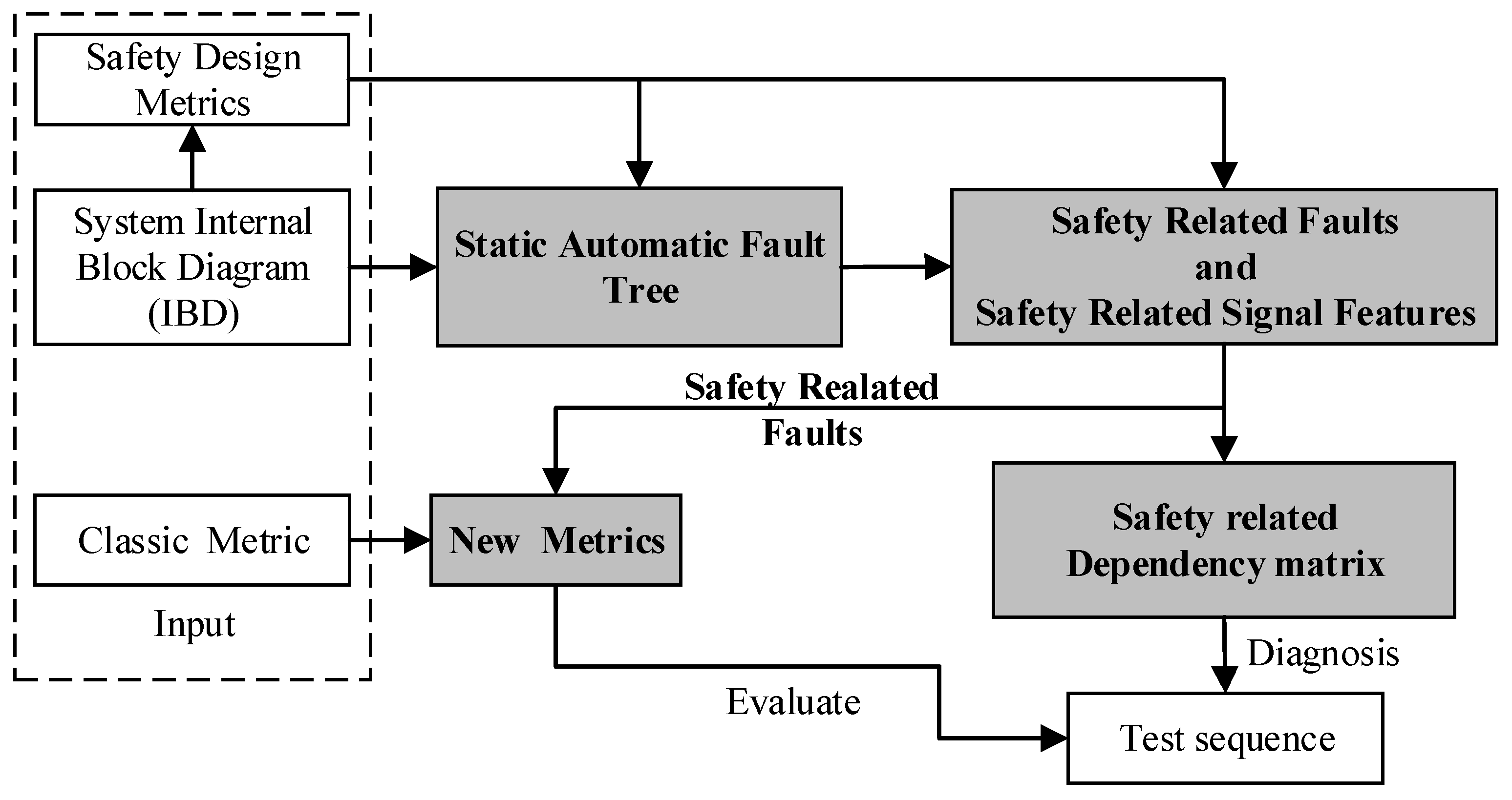
2. Safety-Related Fault Model (SRFM)

2.1. Motivation

To ensure that the test accurately reflects system safety, we must tackle the challenges of quantifying safety and the absence of measurement metrics. The difficulty in quantifying safety within DFT gives rise to two subsidiary challenges: 1. How to quantitatively define safety; and 2. how to establish a correlation with the DFT model after quantitative definition. For the first challenge, this paper draws on FTA. Although FTA can quantitatively depict safety, the traditional manual FTA method is heavily influenced by designers. The Static Automatic FTA (SAFTA) modeling method, grounded in MBSE, significantly reduces human influence and presents a viable solution. For the second challenge, inspiration is taken from the MSFM. Since the modeling results of MSFM do not change the system structure, establishing a mapping relationship based on MBSE facilitates the introduction of the factor about safety. Additionally, insights from the international standard ISO 26262 are incorporated [48]. ISO 26262 categorizes safety-related faults in its initial classification, with sensitivity analysis forming the core of this classification approach, which this paper utilizes to address the challenge. Recognizing the lack of measurement metrics for safety, this paper adopts a straightforward principle, that is, the earlier safety-related fault modes are detected, the better the system safety is reflected. Based on this principle, the test advantage of safety assessment on probability (TASAP) and the test advantage of safety assessment on number (TASAN) are introduced as new measurement indices for the test sequence, resolving the issue of lacking measurement indicators.

2.2. The Whole Picture of SRFM

The whole picture of SRFM is shown in Figure 1. The grey boxes are the newly introduced parts relative to the classic methods.

To ensure that the test sequence accurately reflects system safety, we must address the challenges of quantifying safety and the absence of measurement metrics. Addressing the challenges of quantifying safety means building a new safety-related dependency matrix to generate a test sequence. Addressing the absence of measurement metrics means building new safety-related metrics.

Before building a new safety-related dependency matrix and new metrics, it is necessary to generate safety-related faults (SRF) and safety-related signal features (SRSF). The former is the manifestation of system safety in terms of faults, while the latter is the manifestation of system safety in terms of signal features (tests). Before generating SRF and SRSF, it is necessary to construct a reasonable way to introduce safety factors. This article draws on the idea of sensitivity analysis to analyze the introduction of safety factors through the use of existing safety design metrics and SAFT. SAFT, established from the IBD using the nine-tuples model.

This approach of building new metrics combines traditional metrics with SRF and proposes two new evaluation metrics based on similarity principles.

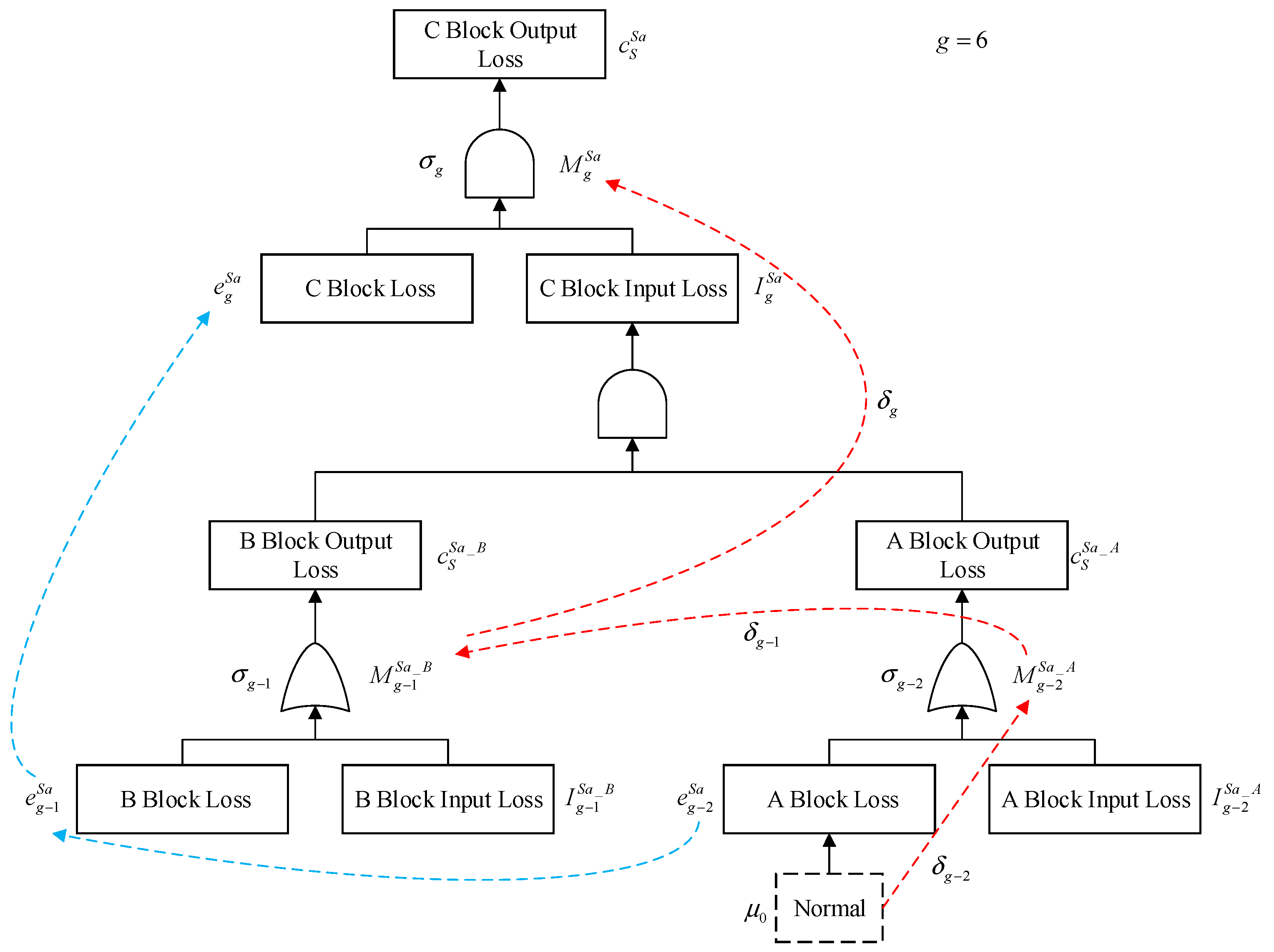
2.3. Static Automatic Fault Tree

To address the challenge of quantitatively introducing safety, the paper uses SAFT to establish a mapping relationship between faults and safety. The nine-tuple model can clearly describe the system state. Therefore, using the nine-tuple model to analyze and establish a static automatic fault tree can clearly describe the relationship between safety and faults. This section mainly elaborates on the process of constructing a fault tree (FT) based on the nine-tuples model. Section 2.3.1 provides fundamental knowledge of nine tuples. The theoretical analysis process of FT modeling from the perspective of pattern change is discussed in Section 2.3.2 by taking a simple series-parallel system as an example. Furthermore, Section 2.3.3 describes the theoretical analysis process of the multi-signal flow model (MSFM) from the perspective of design for testability (DFT). Section 2.3.2 and 2.3.3 show how SAFT can serve as a bridge to connect safety and faults. The specific FT modeling method is outlined in Section 2.3.4.

2.3.1. Fundamental Concepts of Nine Tuples

Let $\mathcal{l}$ be a finite set of constant symbols and $\xi$ be a finite set of variable symbols ($\mathcal{l}\cap \xi =\varnothing$). $\mathcal{l}$ is called a domain. We assume that we provide a mapping from $\xi$ to $2^{\mathcal{l}}$ (the power of $\mathcal{l}$), and then $\forall v\in \xi ,dom\left(v\right)\ne \varnothing$.

$dom\left(v\right)$ is called the domain of the variable $v$, that is, $dom\left(v\right)$ is the set of all possible values of the variable $v$.

Let $\varsigma \subseteq \xi$. We use $dom\left(\varsigma \right)$ to represent the Cartesian product of the domain of variable $\varsigma$: $dom\left(\varsigma \right)={\displaystyle \prod _{v\in \varsigma }dom\left(v\right)}$. In other words, $dom\left(\varsigma \right)$ represents the set of all possible values of variable $\varsigma$. Let $U\in \varsigma$. We define $U\left[v\right]$ as the value of the variable $v$ in the estimator $U$. Define $U\left[v\leftarrow c\right],c\in dom\left(v\right)$, and this estimator is equal. Only when the variable is $v$, its estimator is $c$. Then, nine tuples can be represented as

$$\zeta =〈\mathcal{l},dom,S,{\mathsf{\Gamma }}^{in},{\mathsf{\Gamma }}^{out},\sum ,\delta ,\sigma ,{\mu }_0〉$$

(1)

where,

$\mathcal{l}$ and $dom$ are defined fields and field functions;

$S,{\mathsf{\Gamma }}^{in},{\mathsf{\Gamma }}^{out}$ are three intersecting subsets of $V$. These are the state variables, input flows, and output flows, respectively.

$\sum$ is a finite set of event symbols;

$\delta$ is a partial function that maps $dom\left(S\right)\times dom\left({\mathsf{\Gamma }}^{in}\right)\times \sum$ to $dom\left(S\right)$.$\delta$ provides the next value of the state variable in the case of the current value of the state variable, value of the input flow, and occurrence of the event causing a mode change.

$\sigma$ is a full function mapped from $dom\left(S\right)\times dom\left({\mathsf{\Gamma }}^{in}\right)$ to $dom\left({\mathsf{\Gamma }}^{out}\right)$.$\sigma$ provides the value of the output flow for the current value of the state variable and the value of the input flow.

${\mu }_0$ belongs to $dom\left(S\right)$ and is called the initial state.

2.3.2. The Theoretical Analysis Process

Figure 2 illustrates the IBD for a simple but representative system S, which comprises three blocks, denoted as A, B, and C. The system S is presumed to suffer failure.

Under the single-fault assumption, the elements of nine tuples can be expressed as:

$$\begin{array}{l}\begin{array}{cc}S=\left\{state\_A,state\_B,state\_C\right\}& with\end{array}\\ dom\left(state\_A\right)=\left\{normal,fault\right\},\\ dom\left(state\_B\right)=\left\{normal,fault\right\},\\ dom\left(state\_C\right)=\left\{normal,fault\right\},\\ {\mathsf{\Gamma }}^{in}=\left\{inFlow\_A,inFlow\_B\right\},\\ {\mathsf{\Gamma }}^{out}=\left\{outFlow\_A,outFlow\_B,outFlow\_C\right\},\\ \sum =\left\{\begin{array}{l}A\_normal,B\_normal,C\_normal,\\ A\_fault,B\_fault,C\_fault\end{array}\right\},\\ {\mu }_0=\left\{A\_normal,B\_normal,C\_normal\right\},\end{array}$$

(2)

$\delta$ and $\sigma$ are shown in Figure 3.

Suppose $\zeta =〈\mathcal{l},dom,S,{\mathsf{\Gamma }}^{in},{\mathsf{\Gamma }}^{out},\sum ,\delta ,\sigma ,{\mu }_0〉$ describes a system that may fail, initial state ${\mu }_0$ represents the normal state of the system, $\sum$ represents the fault of the block, Part of $S$ represents the fault, and the path from initial state ${\mu }_0$ to these $S$ represents the fault scenario.

This compilation captured the fault scenario as a set of Boolean equations. This produces the Boolean formula ${\varphi }_{v,c}$. then $\left(v,c\right),v\in S\cup {\mathsf{\Gamma }}^{out},c\in dom\left(v\right)$, then:

(a)

The variable of ${\varphi }_{v,c}$ is $\sum$;

(b)

The minimum cut set of ${\varphi }_{v,c}$ corresponds to the event set $\left\{e_1,\dots e_k\right\}$ one by one, so there is a modal sequence $M_0,\dots M_k$, and $M_0={\mu }_0.$

It can be expressed as:

$$\begin{array}{l}\delta \left(M_0,I_1,e_1\right)=M_1,\dots ,\delta \left(M_{k-1},I_k,e_k\right)=M_k\\ \begin{array}{cc}some& I_1,\dots ,\end{array}{I}_k\in dom\left({\mathsf{\Gamma }}^{in}\right),\\ \sigma \left(M_k,I_k\right)\left[v\right]=c,\end{array}$$

(3)

For the system shown in Figure 2, the initial state is set as

$$M_0={\mu }_0=\left\{\begin{array}{l}A\_normal,\\ B\_normal,\\ C\_normal,\end{array}\right\},$$

(4)

where,

$A\_normal$ denotes that A is in normal state.

$B\_normal$ denotes that B is in normal state.

$C\_normal$ denotes that C is in normal state.

Similarly, $A\_fault$ denotes that A is in fault. $B\_fault$ and $C\_fault$ have similar meanings. As shown in Figure 3, there are seven modes of $M_0,\dots ,M_7$. It should be noted that these seven modes are not modal sequences.

$$\begin{array}{l}{M}_0=\left\{\begin{array}{l}A\_normal,\\ B\_normal,\\ C\_normal,\end{array}\right\},M_1=\left\{\begin{array}{l}A\_fault,\\ B\_normal,\\ C\_normal,\end{array}\right\},M_2=\left\{\begin{array}{l}A\_normal,\\ B\_fault,\\ C\_normal,\end{array}\right\},\\ M_3=\left\{\begin{array}{l}A\_normal,\\ B\_normal,\\ C\_fault,\end{array}\right\},M_4=\left\{\begin{array}{l}A\_fault,\\ B\_fault,\\ C\_normal,\end{array}\right\},M_5=\left\{\begin{array}{l}A\_normal,\\ B\_fault,\\ C\_fault,\end{array}\right\},\\ M_6=\left\{\begin{array}{l}A\_fault,\\ B\_normal,\\ C\_fault,\end{array}\right\},M_7=\left\{\begin{array}{l}A\_fault,\\ B\_fault,\\ C\_fault,\end{array}\right\},\end{array}$$

(5)

There are six events $e_1,\dots ,e_7$ in the system.

$$\left\{\begin{array}{l}{e}_1=A\_fault,e_2=B\_fault,e_3=C\_fault,\\ e_4=A\_normal,e_5=B\_normal,e_6=C\_normal,\end{array}\right.$$

(6)

As shown in Figure 3, there exist six (3!) paths in a fault with $M_7$ at its end.

$$\begin{array}{l}path\_1:M_0\to M_1\to M_4\to M_7,\\ path\_2:M_0\to M_1\to M_6\to M_7,\\ path\_3:M_0\to M_2\to M_4\to M_7,\\ path\_4:M_0\to M_2\to M_5\to M_7,\\ path\_5:M_0\to M_3\to M_5\to M_7,\\ path\_6:M_0\to M_3\to M_6\to M_7,\end{array}$$

(7)

Taking $path\_1$ as an example, the mathematical model of path $M_0\to M_1$ is established as follows.

$$\begin{array}{l}\delta \left(M_0,I_1,e_1\right)=M_1\\ \begin{array}{ll}where& M_0={\mu }_0=\left\{\begin{array}{l}A\_normal,\\ B\_normal,\\ C\_normal,\end{array}\right\},\end{array}\\ I_1=\left\{inFlow\_A\_normal,inFlow\_B\_normal\right\},\\ e_1=\left\{A\_fault\right\},\end{array}$$

(8)

where,

$inFlow\_A\_normal$ denotes that input flow A is in normal state

$inFlow\_B\_normal$ denotes that input flow B is in normal state.

Subsequently:

$$\begin{array}{l}{M}_1=\left\{\begin{array}{l}A\_fault,\\ B\_normal,\\ C\_normal,\end{array}\right\},\\ \sigma \left(M_1,I_1\right)\left[v\right]=\left\{inFlow\_B\right\},\end{array}$$

(9)

Let the Boolean of $e_1$ in $fault$ be 1, and the Boolean in $normal$ be 0; then, the Boolean equation (a minimum cut set) constructed by $path\_1$ can be expressed as ${\varphi }_{v,c}^{path\_1}=e_1{e}_2{e}_3$.

Let $\sigma \left(M_7,I_7\right)\left[v\right]=c_7$ and $M_7$ be considered as the fault at the end of the path, $c_7$ be the output as the fault, and ${\varphi }_{v,c}^{c_7}$ be expressed as (in sequence).

$${\varphi }_{v,c}^{c_7}=e_1{e}_2{e}_3+e_1{e}_3{e}_2+e_2{e}_1{e}_3+e_2{e}_3{e}_1+e_3{e}_1{e}_2+e_3{e}_2{e}_1$$

(10)

The above analysis process can show that the modal change theory based on 9-tuples is suitable for the FTA.

2.3.3. Modal Change Analysis of MSFM Based on Nine Tuples

Considering the multi-signal flow diagram (MSFD) of the system S shown in Figure 4 [5], which is constructed based on its IDB in Figure 2.

The signals within the multi-signal flow diagram (MSFD) are classified based on the impact of module faults on system functions [5]. This aspect primarily focuses on the system’s reliability, assessing whether it is able to operate reliably.

Within the MSFD, faults are classified into two kinds: general faults and functional faults based on their impact on the system. Consequently, each block is augmented with a pair of system states that delineate the fault type, encompassing general and functional faults. This model can be represented using nine tuples as follows:

$$\begin{array}{l}\begin{array}{cc}S=\left\{state\_A,state\_B,state\_C\right\}& with\end{array}\\ dom\left(state\_A\right)=\left\{normal,general\_fault,functional\_fault,others\right\},\\ dom\left(state\_B\right)=\left\{normal,general\_fault,functional\_fault,others\right\},\\ dom\left(state\_C\right)=\left\{normal,general\_fault,functional\_fault,others\right\}\end{array}$$

(11)

The input and output flow can be expressed as follows:

$$\begin{array}{l}{\mathsf{\Gamma }}^{in}=\left\{inFlow\_A,inFlow\_B\right\}\\ \begin{array}{cc}{\mathsf{\Gamma }}^{out}=\left\{outFlow\_A,outFlow\_B,outFlow\_C\right\}& with\end{array}\\ dom\left(inFlow\_A\right)=dom\left(inFlow\_B\right)=\left\{normal,error\right\}\\ dom\left(outFlow\_A\right)=dom\left(outFlow\_B\right)=dom\left(outFlow\_C\right)=\left\{normal,error\right\}\end{array}$$

(12)

Events can be expressed as follows:

$$\begin{array}{l}\sum =\left\{\begin{array}{l}A\_normal,B\_normal,C\_normal,\\ A\_general\_fault,B\_general\_fault,C\_general\_fault\\ A\_functional\_fault,B\_functional\_fault,C\_functional\_fault\end{array}\right\}\\ \begin{array}{cc}with& \sum =\left\{e_1^{Sa},\dots ,e_9^{Sa}\right\}\end{array}\end{array}$$

(13)

The current state can be expressed as $S_N,{\mathsf{\Gamma }}_N^{in}$ or as the compiled result: $M_N,I_N$.

The events that occur in this state can be expressed as an ${\sum }_N$ or as a compiled result: $e_N$.

The next state of the system can be expressed as: $\delta \left(M_N,I_N,e_N\right)$.

According to the properties of the Parallel composition [38], the output flow at $outFlow\_A,outFlow\_B,outFlow\_C$ can be expressed by the function $\sigma$:

$${\sigma }_{outFlow\_A}\left(M_N,I_N\right),{\sigma }_{outFlow\_B}\left(M_N,I_N\right),{\sigma }_{outFlow\_C}\left(M_N,I_N\right)$$

(14)

The output of each block in the MSFD of the system is denoted by the output flow ${\sigma }_{Block\_name}\left(M_N,I_N\right)$. It is worth noting that the fault type of the system is characterised by the current state $M_N$ of the system. ${\varphi }_{v,c}$ can perform reverse engineering through path tracing, the theoretical analysis of which is as follows:

First, a fault was selected. Assuming that $M_g^{Sa}$ is the fault and that the input flow is $I_g^{Sa}$, then $\sigma \left(M_g^{Sa},I_g^{Sa}\right)\left[v\right]=c^{Sa}$, $c^{Sa}$ represents the set of output flows of the block. Taking a simple system S as an example, the set of system output flows $c^{Sa}$ can be expressed as

$$\left\{{\sigma }_{outFlow\_A}^S\left(M_g^{Sa},I_g^{Sa}\right),{\sigma }_{outFlow\_B}^S\left(M_g^{Sa},I_g^{Sa}\right),{\sigma }_{outFlow\_C}^S\left(M_g^{Sa},I_g^{Sa}\right)\right\}$$

(15)

The system fault does not necessitate assessing the output flow of all blocks. Typically, only the output part of the system (as in Block C in Figure 4) requires assessment. Therefore, let us assume that the output flow of the terminal module in the fault is

$$c_S^{Sa}={\sigma }^S\left(M_g^{Sa},I_g^{Sa}\right)$$

(16)

Upon occurrence of the output flow, the system will encounter a fault (corresponding to the top event of FT). Traverse through all combinations of modes and input flows in the preceding stage under that mode. Taking $M_g^{Sa}$ as an example, any path $i$ can be expressed as:

$$M_{g-1}^{Sa}={\delta }_i^{-}\left(M_g^{Sa},I_g^{Sa},e_g^{Sa}\right)$$

(17)

where ${\delta }_i^{-}$ means the inverse mapping of ${\delta }_i$ under the $i$ th path.

Finally, based on the recursive relationship, the Boolean expression for the fault was derived in reverse. Taking $M_g^{Sa}$ as an example, the results are as follows:

$$M_{g-1}^{Sa}={\delta }_i^{-}\left(M_g^{Sa},I_g^{Sa},e_g^{Sa}\right),\dots ,M_0^{Sa}={\mu }_0^{Sa}={\delta }_i^{-}\left(M_1^{Sa},I_1^{Sa},e_1^{Sa}\right)$$

(18)

Using the logical OR of all paths, ${\varphi }_{v,c}$ with $M_g^{Sa}$ as the fault can be obtained. The above analysis demonstrates that the theory based on nine tuples is applicable to the MSFM and the derived models based on the MSFM.

2.3.4. A General Static Automatic Fault Tree Modeling Method

Based on Section 2.3.2 and Section 2.3.3, it can be inferred that using nine tuples as a connection for integrating safety is theoretically sound. Drawing on existing methodologies [41,49,50,51,52], this paper presents a comprehensive static automatic fault tree modeling approach for testability design.

To establish a link between modules and fault trees, the first step is to define the base unit (BU) of SAFT. In the theory of this paper, BU is the basic component of SAFT. This can be conceived as a module mapped onto the fundamental structure of the fault tree. The BU is illustrated in Figure 5.

The BU is mainly comprised of Block Output Loss, Block Loss, and Block Input Loss. Block Output Loss denotes a state where the terminal module experiences output loss. Furthermore, based on the analysis outcomes, the $\sigma$ describes the logical correlation between Block Loss, Block Input Loss, and Block Output Loss, representing the AND/OR gates in the diagram. We term its corresponding gate as the Gate of BU (GBU).

To illustrate the FT modeling process with nine tuples more clearly, let us consider an example with system S:

The top event of the FT is selected as “The output flow of S fault is $c_S^{Sa}$.”. For simplicity, we will refer to it as “C Block Output Loss”. The BU of the top event is depicted in Figure 6.

According to the definition of BU in the nine tuples, the FT constructed using S as an example is shown in Figure 7.

In Figure 7, GBU represent $\sigma$, and for ease of understanding, the mode $M^{Sa}$ in which the system is located is also represented here. “Block Loss” represents the basic event $e^{Sa},e^{Sa}\in \sum$. “Block Input Loss” represents the input stream $I^{Sa},I^{Sa}\in dom\left({\mathsf{\Gamma }}^{in}\right)\cup dom\left({\mathsf{\Gamma }}^{out}\right)$. The red dashed line signifies the virtual system’s modal changes. Meanwhile, the blue dashed line denotes the corresponding sequence of events. The modal change process corresponds to the element $\delta$. The mathematical depiction of path tracing is as follows:

$$\begin{array}{l}{M}_5^{Sa}={\delta }_6^{-}\left(M_6^{Sa},I_6^{Sa},e_6^{Sa}\right)\\ M_4^{Sa}={\delta }_5^{-}\left(M_5^{Sa},I_5^{Sa},e_5^{Sa}\right)\\ {\mu }_0^{Sa}=M_3^{Sa}={\delta }_4^{-}\left(M_4^{Sa},I_4^{Sa},e_4^{Sa}\right)\end{array}$$

(19)

In Figure 7, the gates within the basic unit mirror those in the nine tuple, and for clarity, the system’s current mode is also depicted. “Block Loss” signifies the basic event, while “Block Input Loss” represents the input stream. The red dashed line illustrates the virtual system’s modal changes (although static FTs do not require event ordering), whereas the blue dashed line indicates the sequential order of events. The modal change process aligns with the element $\delta$. The mathematical representation of path tracing is as follows:

Therefore, the ${{\varphi }^{\prime }}_{v,c}$ can be expressed as (in order):

$${{\varphi }^{\prime }}_{v,c}=\left(e_6^{Sa}{I}_6^{Sa}\right)=\left(e_6^{Sa}\left(e_5^{Sa}+I_5^{Sa}\right)\left(e_4^{Sa}+I_4^{Sa}\right)\right)$$

(20)

Among them, “( )“ represents the Boolean representation of the output event of a BU.

Suppose without loss of generality that the external input flow does not have any errors.

Then,

$$dom\left(inFlow\_A\right)=dom\left(inFlow\_B\right)\notin \sum$$

(21)

$$\left\{inFlow\_A=normal,inFlow\_B=normal\right\}$$

(22)

Then, ${{\varphi }^{\prime }}_{v,c}$ can be simplified as

$${{\varphi }^{\prime }}_{v,c}=\left(e_6^{Sa}{I}_6^{Sa}\right)=\left(e_6^{Sa}\left(e_5^{Sa}+0\right)\left(e_4^{Sa}+0\right)\right)=e_6^{Sa}{e}_5^{Sa}{e}_4^{Sa}$$

(23)

$e_6^{Sa},e_5^{Sa},e_4^{Sa}$ correspond one-to-one to $e_3,e_2,e_1$, and the results of ${{\varphi }^{\prime }}_{v,c}$ are exactly one of the subsets (in order) of the set of results in ${\varphi }_{v,c}^{c_7}$. It proves the effectiveness of using path tracing to construct FTs.

To further clarify the relationship between the theoretical model and FT. The correspondence between the FT of S and elements of ${{\varphi }^{\prime }}_{v,c}$ is shown in Figure 8.

The dashed box in Figure 8 represents the BU, and the entire FT consists of two parts: Stage and Gate. Stage delineates the hierarchy of the FT; for example, $\left(e_6^{Sa}{I}_6^{Sa}\right)$ corresponds to the hierarchy of the top event, known as Stage 1; $\left(e_5^{Sa}+I_5^{Sa}\right),\left(e_4^{Sa}+I_4^{Sa}\right)$ corresponds to the level of the subsequent event, identified as Stage 2, and so forth. Gate indicates the relationship between the upper BU and the lower BU, aligning with the assertion proposed in [52]. Stage 1 and Stage 2 correspond to Gate 1. Stage 2 and Stage 3 correspond to Gate 2, and so on. The gate within the base unit (BU) is called GBU, while the gate between BUs is known as the Gate of Stage (GS). GS is characterized by a single state: “AND”. This is mainly because the transformation of the typical SysML model into an automatic static fault tree results in only one state. The modeling results of the typical fault tree corresponding to the SysML model are shown in Figure 9.

In summary, the mapping relationship between the nine tuples and their fault trees has been comprehensively discussed. It is important to see that the construction of GBU and GS corresponds to two pivotal mapping parameters $\sigma$ and $\delta$. Most sources optimize these two parameters [33,34,52], but often without considering safety aspects. We divide GBU into “AND” and “OR” Gates, while GS is restricted to “AND” only. This arrangement effectively illustrates the relationship between the fault tree and MSFD, ensuring a straightforward logical structure for the fault tree and simplifying the theoretical analysis for subsequent testability modeling.

2.4. Safety-Related Faults and Safety-Related Signal Features

This section mainly introduces safety-related faults (SRF) and safety-related signal features (SRSF). These components are the basis of the dependency matrix proposed in the study and are used for constructing the safety dependency D matrix (S-D matrix). The key idea can be summarized as follows: when the occurrence probability of top events related to safety is affected by basic events (including intermediate and bottom events), leading to a failure to meet safety design requirements, it constitutes an SRF. The signal features affected by SRF are called SRSF.

To assess the impact of events on the occurrence probability of top events, safety sensitivity is introduced based on global sensitivity [53]. The difference between safety sensitivity and global sensitivity lies in the absence of absolute values in safety sensitivity. This is because a reduction in the occurrence probability of safety-related top events indicates an improvement in safety.

The definition of safety sensitivity is provided in Section 2.4.1, while the calculation methods for SRF and SRSF are outlined in Section 2.4.2.

2.4.1. Safety Sensitivity

Supposing that the probability density distribution function of random input variables can be expressed as $\rho \left(\mathbf{X}\right)$, the fault probability can be expressed as $P\left(\mathbf{X}\right)$, and the model of fault tree can be expressed as $Y={{\varphi }^{\prime }}_{v,c}\left(\mathbf{X}\right)$. Note that the unconditional fault probability value of $Y$ is $P_{f_Y}$. Note that the theoretical safe fault probability value of $Y$ is $P_{f_Y}^{*}$. When the basic variable $X_i$ takes its present value $x_i^{*}$, the conditional probability value of $Y$ is $P_{\left.f_Y\right|X_i}$. As the elimination of $X_i$ uncertainty will affect the fault probability, there will be some differences between $P_{f_Y}$ and $P_{\left.f_Y\right|X_i}$. Considering the influence of $X_i$ on fault probability when it changes in its domain, safety sensitivity which can reflect the influence of basic variable $X_i$ on fault probability is established.

The designed safety sensitivity (DSS) ${\eta }_i$ is defined as the $X_i$ versus the unconditional fault probability $P_{f_Y}$, which is expressed as follows:

$${\eta }_i={\displaystyle {\int }_{-\infty }^{+\infty }\left(P_{\left.f_Y\right|X_i}-P_{f_Y}\right)\rho \left(X_i\right)}d{X}_i$$

(24)

The theoretical safety sensitivity (TSS) ${\eta }_{{}_i}^{\ast }$ is defined as $X_i$ while the unconditional fault probability $P_{f_Y}^{*}$, and is expressed as follows:

$${\eta }_{{}_i}^{\ast }={\displaystyle {\int }_{-\infty }^{+\infty }\left(P_{\left.f_Y\right|X_i}-P_{f_Y}^{*}\right)\rho \left(X_i\right)}d{X}_i$$

(25)

Comparing the definitions of ${\eta }_i$ and ${\eta }_{{}_i}^{\ast }$, ${\eta }_{{}_i}^{\ast }$ is related to standard values, whereas ${\eta }_i$ is related to design values. Owing to the requirement of maintaining a certain safety threshold for system design, selecting the DSS as the evaluation parameter has higher requirements. The DSS was chosen as the evaluation parameter. Safety sensitivity has the following characteristics. Because the top event is related to safety, we achieve the following sub cases: 1. if ${\eta }_i\ge 0$, the input variable $X_i$ has no impact on system safety. 2. If ${\eta }_i<0$, the input variable $X_i$ has an impact on system safety, and the smaller the value, the greater the impact on safety. Safety sensitivity represents the influence of the random variable value rule on system safety and can measure the contribution of each input variable.

2.4.2. Calculation of SRF and SRSF

If any event in the fault tree, other than the top event, is considered a random variable, then any event can be used to calculate the design safety sensitivity (DSS) according to Equation (24). According to the structure of the 0/1 FT, these events only exist in two states: occurrence ($X_i=1$) and non-occurrence ($X_i=0$). Then, the DSS can be expressed as:

$${\eta }_i=P_{\left.f_Y\right|X_i=0}\times P\left(X_i=0\right)+P_{\left.f_Y\right|X_i=1}\times P\left(X_i=1\right)-P_{f_Y}$$

(26)

The calculation of DSS for the input variable $X_i$ is illustrated by the FT shown in Figure 10:

Considering Figure 10 as an example, the DSS can be calculated as follows:

$$\begin{array}{l}{\eta }_1=P\left(X_1=1\right)\times P\left(1\cap X_2\right)+P\left(X_1=0\right)\times P\left(0\cap X_2\right)-P_{f_Y}\\ =P\left(X_1=1\right)\times \left(P\left(X_4\right)+P\left(X_5\right)+P\left(X_6\right)\right)\times \left(P\left(X_8\right)+P\left(X_9\right)\right)-P_{f_Y}\\ ......\end{array}$$

(27)

The faults are shown in the block loss of the base unit (BU). In all the aforementioned cases, only the normal or the fault state of the block is described. In practical applications, block loss may involve multiple faults. Incorporating these into the fault tree can ensure that the test results can measure the system’s safety more accurately. The BU with N faults is illustrated in Figure 11.

The faults in the module correspond to Block Loss. Therefore, the SRF only needs to analyze the sensitivity of the Block Loss in BU. If the DSS of the input variable $X_i\left(i\ge 1\right)$ corresponds to module M, then the Fault of $X_i\left(i\ge 1\right)$ is the SRF. Unlike SRF, module faults may not necessarily affect signal features; therefore, it is necessary to analyze the impact of specific faults on signal features. Referring to the idea of a module fault causing signal changes in the MSFM [5], the design judgment criterion is as follows. If the occurrence of a fault causes a change in the signal feature, then the signal feature is considered an SRFS.

Considering ${\eta }_4$ in Figure 10 as an example of the process of establishing the SRF and SRSF:

$$\begin{array}{l}{\eta }_4=P\left(X_1\right)\times \left(P\left(X_8\right)+P\left(X_9\right)\right)\times \left(P\left(X_4=1\right)\times P\left(1\cup X_5\cup X_6\right)+P\left(X_1=0\right)\times P\left(0\cup X_5\cup X_6\right)\right)-P_C^{*}\\ =P\left(X_1\right)\times \left(P\left(X_8\right)+P\left(X_9\right)\right)\times \left(P\left(X_4=1\right)+P\left(X_4=0\right)\times P\left(X_5\right)\times P\left(X_6\right)\right)\end{array}$$

(28)

In (28), $P\left(X_1\right)$,$P\left(X_4\right)$,$P\left(X_5\right)$,$P\left(X_6\right)$,$P\left(X_8\right)$, and $P\left(X_9\right)$ are all known prior probabilities. If ${\eta }_4<0$, then the B-1 block loss is the SRF, otherwise it is not. If there is an SRF in Module B, a specific analysis can be conducted to determine the SRSF.

2.5. Safety-Related Dependency Matrix (S-D Matrix)

When using the classic multi-signal flow model (MSFM) to construct the dependency matrix, from a reliability perspective, the fault of a module is classified into two types: functional faults and general faults. The safety-related dependency matrix (S-D matrix) proposed in this article introduces two additional elements, safety-related faults (SRF) and safety-related signal features (SRSF), from a safety perspective. Consequently, when forming an S-D matrix for a system, fault types for any module will be classified into four categories: 1. Functional and Safety-related Fault (FFS); 2. Functional and Non-safety-related Fault (FFN); 3. General and Safety-related Fault (FGS); 4. General and Non-safety-related Fault (FGN).

The rows and columns of the S-D matrix define the relationship between faults and tests. Signal features are then designed to establish a link between safety-related faults and tests. These features exhibit a one-to-one or many-to-one correspondence with the test, implying that the test indirectly examines the fault through the assessment of the signal features (or SRSF). One test may correspond to multiple signal features. A practical concern thus arises: determining whether detected signal features indicate the detection of the associated fault. The currently commonly accepted assumption is that detecting the signal features related to the fault signifies detecting the fault itself [5]. The S-D matrix proposed in this study still adheres to this assumption.

In summary, establishing the S-D matrix involves the following key steps: 1. Classifying faults into functional and general types; 2. Using the proposed SRF to further classify faults into safety and non-safety types and provide the corresponding SRSF; 3. Formulating an S-D matrix with modules as rows and tests (incorporating SRSF) as columns.

2.6. New Metrics

Since critical fault (for safety) and general fault are not discriminated in traditional testable design, the general metrics are thus not enough anymore to measure safety-critical systems (SCS). To this end, the paper proposes the Test Advantage of Safety Assessing on Probability (TASAP), to evaluate the diagnosis result of SCS. The test sequencing problem involves finding the optimal test sequence with the maximum TASAP and the maximum TASAN.

The TASAP is defined as follows:

$$J_{TASAP}={\displaystyle \sum _{i=0}^m\left(\frac{1}{{\displaystyle \sum _{T_j\in T_{f_i^S}}{l}_j}}\right)}p\left(f_i^S\right),$$

(29)

where,

$T_j$ is the $j$-th test;

$l_j$ is the test cost of $T_j$;

$f_i^S$ is the $i$-th safety related fault;

$T_{f_i^S}$ is the test sequence of $f_i^S$, when $f_i^S$ is detected;

$p\left(f_i^S\right)$ is a priori probability after $f_i^S$ normalization.

$m$ is the number of all fault modes.

The TASAN is defined as follows:

$$J_{TASAN}=,{\displaystyle \sum _{T_j\in T_{f_i^S}}{\displaystyle \sum _{i=0}^m\left(\frac{l_j}{m}\right)}}$$

(30)

where,

$T_j$ is the $j$-th test;

$l_j$ is the test cost of $T_j$;

$f_i^S$ is the $i$-th safety-related fault;

$T_{f_i^S}$ is the test sequence of $f_i^S$, when $f_i^S$ is detected;

$m$ is the number of all fault modes.

According to (29), TASAP is mainly related to two parameters, one is the prior probability $p\left(f_i^S\right)$ and the other is the test cost $l_j$. The lower the test cost and the higher the probability of occurrence after measuring $f_i^S$, the greater the value. On the contrary, the smaller it is. Therefore, when the test costs are the same, the larger the TASAP value, the greater the probability of fault affecting safety occurring and being detected earlier.

Similarly, according to (30), TASAN is mainly related to two parameters: the proportion of faults that affect safety to the total number of faults ${\displaystyle \sum _{i=0}^m\left(\frac{1}{m}\right)}$, and the test cost $l_j$. The earlier the testing round, the lower the testing cost, and the more faults that affect safety are measured, the greater the value. On the contrary, the smaller it is. Therefore, when the test cost is the same, the larger the TASAN value, the earlier the more faults that affect safety are detected.

Both of these metrics can achieve the evaluation of safety by testing sequences. The difference is that TASAP mainly focuses on the probability of occurrence of faults that affect safety, while TASAN mainly focuses on the number of faults that affect safety. The similarity is that both focus on the sorting of faults that affect safety, as well as the test cost. Therefore, for systems that cannot provide accurate prior probabilities (or in the early stages of design), using TASAN is more reasonable. For systems that can provide accurate prior probabilities (or in the later stages of design), using TASAP is more reasonable. For the ESA, the article has calculated both metrics.

3. Experimental Section

This section evaluates the proposed safety-related fault model (SRFM) by performing a multi-signal flow model (MSFM, special informational flow model) on an electronic safety and arming device (ESA) [54]. Since ESA [55] is a typical and widely used safety-critical system (SCS) with only two critical fault modes—early or late explosion—it is straightforward yet sufficiently representative.

3.1. Experiment Setup

The experiment consists of two main phases: the testability modeling process and the fault diagnosis process. The former involves establishing the D matrix based on the general modeling method and the S-D matrix based on the safety-related fault model (SRFM). The latter includes generating a test sequence after processing the D matrix and S-D matrix using classical fault diagnosis algorithms.

Evaluation is conducted by comparing the output test sequence, fault detection rate (FDR), expected test cost (ETC), test advantage number for safety assessment (TASAN), and test advantage probability for safety assessment (TASAP) between the existing model and SRFM.

• Testability Modeling Process

The general modeling method only focuses on reliability and thus only requires the internal block diagram (IBD) of the ESA. In contrast, the safety-related fault model (SRFM) takes both safety and reliability into account and requires not only the IBD but also safety design metrics. The safety design metrics for ESA can be derived from MIL-STD-1316F “FUZE DESIGN, SAFETY CRITERIA FOR”.

2.

Fault Diagnosis Process

Selection of Test Cost: To measure the accuracy of safety assessment, it is assumed that the test cost for each test is uniform and set at 1.

Selection of Prior Probability: The prior probability in the fault tree (FT) is calculated using GJB/Z299C-2006 [48] “Reliability Prediction Handbook Electronic Equipment”. For prior probabilities not included in the FT, refer to reference [56]. Lightning stroke and other highly unique cases will require special calculations.

Selection of Processing Algorithm: Existing fault diagnosis algorithms often overlook the actual significance of the object and neglect safety considerations. Therefore, this study chooses the two most widely used algorithms: information gain (IG) [54] and weighted fault diagnosis (WFD) [57].

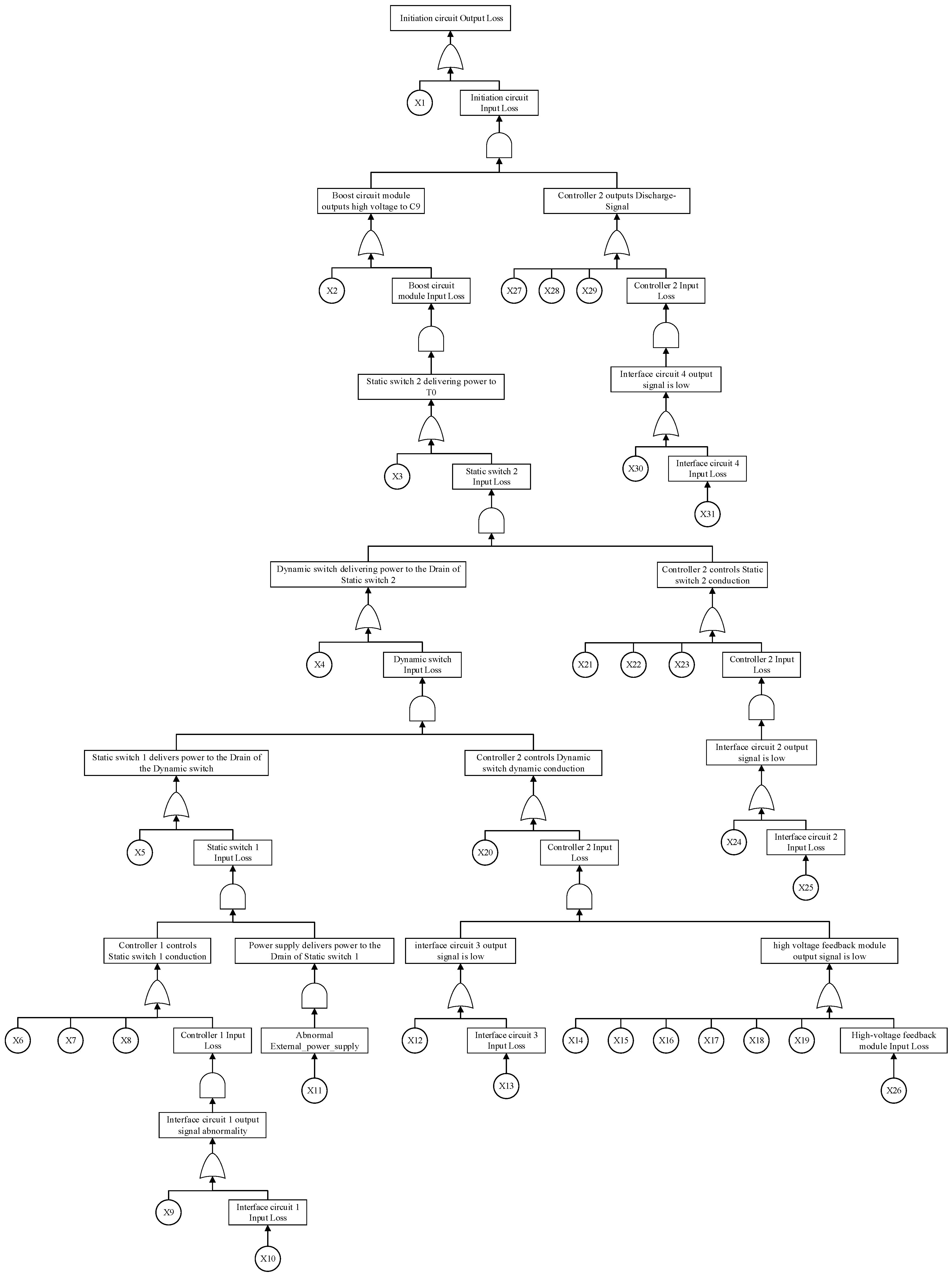
3.2. Electronic Safety and Arming

The signal features of the ESA are selected based on system functionality. The functional structure diagram and multi-signal flow diagram (MSFD) are shown in Figure 12. The signal features are as follows:

• Power supply function: S1 logic power supply signal, S2 power supply signal.
• Logic control functions: S3 static switch 1 status signal, S4 static switch 2 status signal, S5 dynamic switch status signal, and S9 energy circuit conduction signal.
• Circuit boost function: S6 high-voltage capacitor voltage steady-state value and S7 high-voltage capacitor voltage boost speed.
• Trigger function: S8 ignition signal.

Figure 12. The functional structure diagram and multi-signal flow diagram of ESA.

Figure 12. The functional structure diagram and multi-signal flow diagram of ESA.

Taking the ESA illustrated in Figure 12 as an example, the process of establishing the Safety-Related Fault Model (SRFM) can be described as follows:

• Establishing the Static Automatic Fault Tree (SAFT)

Determining the top event: In accordance with the “Safety system failure rate” requirements outlined in Section 3.3 of MIL-STD-1316F “FUZE DESIGN, SAFETY CRITERIA FOR”, the top event identified by the system at the initial stage “Prior to intentional initiation of the arming sequence” is: “fuze de-isolation or action”. According to SRFM, “fuze de-isolation or action” pertains to the output event of the initiation circuit module. For ease of understanding, it is referred to as “initiation circuit function”.

Achievements: Using the ESA as an example, the process of transforming the modular automatic fault tree into an actual fault tree is outlined in detail in Supplementary Materials. The resulting actual fault tree is presented in Figure 13.

2.

Calculating the result of Safety-Related Faults (SRF) and Safety-Related Signal Features (SRSF)

All components of the ESA, except the Explosive Function Initiator (EFI), are electronic components. Therefore, the probability of the bottom event shown in

Table 1. Bottom event of fault tree and its occurrence probability.

Code	Description	$\mathbf{Fault} \mathbf{Probability} \mathbf{(}\times {\mathbf{10}}^{\mathbf{-}\mathbf{3}}\mathbf{)}$	${\mathit{\eta }}_{\mathit{i}}$
X1	Unexpected function of EFI due to lightning stroke	0.0001	−2.632 × 10−7
X2	D3 accidentally outputs high voltage due to lightning stroke	0.0001	0
X3	Static switch 2 fault causes constant continuity between source and drain	7.35	−9.678 × 10−10
X4	Dynamic switch fault causes constant continuity between source and drain	7.35	−9.678 × 10−10
X5	Static switch 1 fault causes constant continuity between source and drain	7.35	0
X6	Photocoupler 6 in controller 1 is damaged, resulting in constant continuity of emitter and collector	0.801	0
X7	Chip fault in controller 1 causes IO_8_E7 constant output low	0.801	0
X8	Chip program error in controller 1 causes IO_8_E7 constant output low	0.801	0
X9	High output due to photocoupler 2 fault in interface circuit 1	1.77	0
X10	Abnormal Order_1 signal	0.058	0
X11	Abnormal External_power_supply	0.058	0
X12	High output due to photocoupler 4 fault in interface circuit 3	1.77	0
X13	Abnormal Order_3 signal	0.058	0
X14	Constant high output caused by operational amplifier 1 fault	1.593	0
X15	Constant low output caused by operational amplifier 2 fault	1.593	0
X16	R31 short circuit	0.058	0
X17	R32 open circuit	0.058	0
X18	R29 short circuit	0.058	0
X19	R30 open circuit	0.058	0
X20	High and low of port IO_8_B9 output dynamic change caused by chip program error in controller 2	0.801	0
X21	Driver chip 2 fault in controller 2 causes out port to output differential signal	0.801	−1.709 × 10−10
X22	Chip fault in controller 2 causes IO_8_B6 constant output low	0.801	−1.709 × 10−10
X23	Chip program error in controller 2 causes IO_8_B6 constant output low	0.801	−1.709 × 10−10
X24	High output due to photocoupler 3 fault in interface circuit 2	1.77	−2.710 × 10−10
X25	Abnormal Order_2 signal	0.058	0
X26	Abnormal feedback signal of the initiation circuit	0.0001	0
X27	Driver chip 2 fault in controller 2 causes out port to output differential signal	0.801	−1.709 × 10−10
X28	Chip fault in controller 2 causes IO_8_B6 constant output low	0.801	−1.709 × 10−10
X29	Chip program error in controller 2 causes IO_8_B6 constant output low	0.801	−1.709 × 10−10
X30	High output due to photocoupler 5 fault in interface circuit 4	1.77	−2.710 × 10−10
X31	Abnormal Order_4 signal	0.058	0

can be estimated according to GJB/Z299C-2006 “Reliability Prediction Handbook Electronic Equipment” [58].

The fault probability of small probability events related to lightning strikes is set to one in ten million (10⁻⁷). There are two reasons for this:

• The probability of lightning striking the equipment using the ESA is generally one in hundreds of thousands. It is nearly impossible for lightning to penetrate the external shell of the equipment and affect the internal capacitance.
• If the feedback signal of the initiation circuit is abnormal, it is necessary to ensure that the high-voltage capacitor in the initiation circuit is charged.

This situation can only occur when the top event happens. This process is a loop. However, in the initial calculation of the occurrence probability of the top event, only a lightning strike can cause an abnormal feedback signal. Therefore, the probability of “abnormal feedback signal of the initiation circuit” is set to one in ten million.

The occurrence probability of all FT bottom events and the corresponding DSS ${\eta }_i$ are shown in Table 1. Generally speaking, if constraints are not added, nearly all events will lead to reduced safety. However, if the reduced value is close to 0, it can be considered that it has no impact on safety. In the study, the fault with a reduction of ${\eta }_i$ less than 10 billionths ($>-1\times {10}^{-10}$) is regarded as having no impact on Safety (${\eta }_i=0$).

3.

Establishment of safety-related dependency matrix (S-D matrix)

To establish the S-D matrix for ESA, in addition to the relationship between tests and signal features in

Table 2. SRF and corresponding SRSF.

Module Code	Safety-Related Faults	Safety-Related Signal Features
M7	Unexpected function of EFI due to lightning stroke	S6
M8	High output due to photocoupler 3 fault in interface circuit 2	S5
M10	High output due to photocoupler 5 fault in interface circuit 4	S8
M11	Driver chip 2 fault in controller 2 causes out port to output differential signal	S8
	Chip fault in controller 2 causes IO_8_B6 constant output low	S8
	Chip program error in controller 2 causes IO_8_B6 constant output low	S8
M12	Dynamic switch fault causes constant continuity between source and drain	S5,S7
M13	Static switch 2 fault causes constant continuity between source and drain	S4,S7

, the following data should be given in particular:

All faults: including both safety-related faults (see

Table 3. Safety-related dependency matrix of ESA.

		T1	T2	T3		T4		T5		T6			T7		T8			T9	T10	$\mathbf{Fault} \mathbf{Probability} (\times {10}^{-3})$
		S1	S2	S1	S3	S1	S5	S1	S4	S1	S2	S6	S1	S8	S1	S5	S6	S7	S9
F1GN	M1	1	0	1	1	1	1	1	1	1	0	1	1	1	1	1	1	1	1	0.74
F2GN	M2	0	1	0	1	0	1	0	1	0	1	1	0	1	0	1	1	1	1	0.38
F3GN	M3	0	0	0	1	0	0	0	0	0	0	1	0	0	0	0	1	0	0	0.62
F4GN	M4	0	0	0	1	0	0	0	0	0	0	1	0	0	0	0	1	0	0	0.40
F5GN	M5	0	0	0	1	0	0	0	0	0	0	1	0	0	0	0	1	0	0	0.95
F5FN		0	0	0	0	0	0	0	0	0	0	0	0	0	0	0	0	0	1	0.82
F6GN	M6	0	0	0	0	0	0	0	0	0	0	1	0	0	0	0	1	0	0	0.18
F6FN		0	0	0	0	0	0	0	0	0	0	0	0	0	0	0	0	1	0	0.56
F7GN	M7	0	0	0	0	0	0	0	0	0	0	1	0	0	0	0	1	0	0	0.12
F7GS		0	0	0	0	0	0	0	0	0	0	1	0	0	0	0	1	0	0	0.0001
F7FN		0	0	0	0	0	0	0	0	0	0	0	0	0	0	0	0	1	0	0.79
F8GN	M8	0	0	0	0	0	1	0	0	0	0	1	0	0	0	0	1	0	0	0.23
F8GS		0	0	0	0	0	1	0	0	0	0	0	0	0	0	0	0	0	0	1.8
F9GN	M9	0	0	0	0	0	0	0	1	0	0	1	0	0	0	0	1	0	0	0.52
F10GN	M10	0	0	0	0	0	0	0	0	0	0	0	0	1	0	0	0	0	0	0.96
F10 GS		0	0	0	0	0	0	0	0	0	0	0	0	1	0	0	0	0	0	1.8
F11GN	M11	0	0	0	0	0	1	0	1	0	0	1	0	0	0	1	1	0	0	0.45
F11 GS1		0	0	0	0	0	0	0	0	0	0	0	0	1	0	0	0	0	0	0.80
F11 GS2		0	0	0	0	0	0	0	0	0	0	0	0	1	0	0	0	0	0	0.80
F11 GS3		0	0	0	0	0	0	0	0	0	0	0	0	1	0	0	0	0	0	0.80
F11FN		0	0	0	0	0	0	0	0	0	0	0	0	1	0	0	0	1	0	0.81
F12GN	M12	0	0	0	0	0	1	0	0	0	0	1	0	0	0	0	1	0	0	0.16
F12GS		0	0	0	0	0	1	0	0	0	0	0	0	0	0	0	0	1	0	7.3
F12FN		0	0	0	0	0	0	0	0	0	0	0	0	0	0	0	0	0	1	0.59
F13GN	M13	0	0	0	0	1	0	0	0	0	0	1	0	0	0	0	1	0	0	0.12
F13GS		0	0	0	0	0	0	0	1	0	0	0	0	0	0	0	0	1	0	7.3
F13FN		0	0	0	0	0	0	0	0	0	0	0	0	0	0	0	0	0	1	0.33
F14GN	M14	0	0	0	0	0	1	0	0	0	0	1	0	0	0	0	1	0	0	0.38

F_XGN, F_XGS represents the general fault of module X, and F_XFN, F_XFS represents the functional fault of module X. (X refers to the numerical subscripts 1, 2,...,14.)

) and non-safety-related faults. The final generated fault and its probability are shown in Table 1. Due to the rough classification of general faults and functional faults, the prior probability cannot be accurately obtained. In addition to the base event and occurrence probability shown in Figure 13 and Table 1, the prior probability of faults in other modules is based on the data given in the previous work [56].

• The SRSF are shown in Table 2.
• The fault modes of the ESA are shown in Table 3.
• Test cost: the test cost represents the cost of each test [57]. It is set to 1.

Finally, for the ESA, this paper establishes two matrices. The D matrix established by classical methods (to be exact, it is MSFM), as shown in

Table 4. Classic dependency matrix of ESA.

		T1	T2	T3		T4		T5		T6			T7		T8			T9	T10
		S1	S2	S1	S3	S1	S5	S1	S4	S1	S2	S6	S1	S8	S1	S5	S6	S7	S9
F1G	M1	1	0	1	1	1	1	1	1	1	0	1	1	1	1	1	1	1	1
F2G	M2	0	1	0	1	0	1	0	1	0	1	1	0	1	0	1	1	1	1
F3G	M3	0	0	0	1	0	0	0	0	0	0	1	0	0	0	0	1	0	0
F4G	M4	0	0	0	1	0	0	0	0	0	0	1	0	0	0	0	1	0	0
F5G	M5	0	0	0	1	0	0	0	0	0	0	1	0	0	0	0	1	0	0
F5F		0	0	0	0	0	0	0	0	0	0	0	0	0	0	0	0	0	1
F6G	M6	0	0	0	0	0	0	0	0	0	0	1	0	0	0	0	1	0	0
F6F		0	0	0	0	0	0	0	0	0	0	0	0	0	0	0	0	1	0
F7G	M7	0	0	0	0	0	0	0	0	0	0	1	0	0	0	0	1	0	0
F7F		0	0	0	0	0	0	0	0	0	0	0	0	0	0	0	0	1	0
F8G	M8	0	0	0	0	0	1	0	0	0	0	1	0	0	0	0	1	0	0
F9G	M9	0	0	0	0	0	0	0	1	0	0	1	0	0	0	0	1	0	0
F10G	M10	0	0	0	0	0	0	0	0	0	0	0	0	1	0	0	0	0	0
F11G	M11	0	0	0	0	0	1	0	1	0	0	1	0	0	0	1	1	0	0
F11F		0	0	0	0	0	0	0	0	0	0	0	0	1	0	0	0	1	0
F12G	M12	0	0	0	0	0	1	0	0	0	0	1	0	0	0	0	1	0	0
F12F		0	0	0	0	0	0	0	0	0	0	0	0	0	0	0	0	0	1
F13G	M13	0	0	0	0	1	0	0	0	0	0	1	0	0	0	0	1	0	0
F13F		0	0	0	0	0	0	0	0	0	0	0	0	0	0	0	0	0	1
F14G	M14	0	0	0	0	0	1	0	0	0	0	1	0	0	0	0	1	0	0

F_XG represents the general fault of module X, and F_XF represents the functional fault of module X. (X refers to the numerical subscripts 1, 2,...,14.)

. The S-D matrix established by using SRFM, as shown in

Table 5. Test of ESA.

Test	Description (A Means the Analogue Quantity, D Means the Digital Quantity)	Corresponding Signal Feature Number
T1	Test the logic power supply signal level (A)	1
T2	Test the power supply signal level (A)	2
T3	Test the control signal level output from controller 1 to static switch 2 (D)	1,3
T4	Test the control signal level output from controller 2 to dynamic switch (D)	1,5
T5	Test the control signal level output from controller 2 to static switch 2 (D)	1,4
T6	Test the output voltage value of the boost circuit module (A)	1,2,6
T7	Test the control signal level output from controller 2 to the initiation circuit (D)	1,8
T8	Test the feedback voltage signal of high-voltage feedback module (D)	1,5,6
T9	Test the dynamic switch output signal (voltage or current can be used) (A)	7
T10	Test the output signal (voltage or current) of static switch 2 (A)	9

.

3.3. Results and Analysis

The benefits are demonstrated through experiments. The D matrix and S-D matrix proposed in the paper are applied to the ESA, and then classical dependency matrix processing algorithms are used for fault diagnosis. The controlled variables include the object and processing method, while the assessment parameters include fault detection rate (FDR), expected test cost (ETC), test advantage probability for safety assessment (TASAP), and test advantage number for safety assessment (TASAN). The termination condition for matrix processing is set to detect all faults. The results are presented in

Table 6. Comparison results of D matrix and S-D matrix processed by IG and WFD.

Object	Processing Method	Test Sequence	FDR	ETC	TASAP	TASAN
S-D	WFD	T8→T7→T9→T10→T4	100%	2.6376	0.2386	0.7143
	IG	T9→T7→T6→T4→T10	100%	1.8395	0.5584	0.6071
D	WFD	T8→T9→T10→T7	100%	1.9199	0.1306	0.45
	IG	T8→T9→T7→T10	100%	1.8427	0.1385	0.40

.

It can be observed from Table 6 that the advantages of SRFM are mainly evident in:

• Improvement in TASAP: By comparing the S-D matrix and D matrix established for the ESA, when WFD is used as the processing algorithm, the TASAP of the former increases by 82%, and when IG is used, it increases by 303%. This indicates that the test sequence generated by the S-D matrix significantly enhances the system safety evaluation.
• Enhancement in TASAN: The S-D matrix and D matrix established for the ESA show an improvement in TASAN. With WFD, the former increases by 59%, and with IG, it increases by 52%. This reinforces the idea that the test sequence derived from the S-D matrix improves system safety evaluation.
• IG’s ETC remains largely unchanged: When IG is used as the processing algorithm, the ETC of the S-D matrix is reduced by only 0.0148 compared to the D matrix. This suggests that the ETC generated by the S-D matrix’s test sequence is comparable to or insignificantly different from that generated by the D matrix as measured by the ETC standard.
• Both WFD and IG achieve a 100% FDR: Using the ESA as the subject, it is clear that employing the S-D matrix for diagnostic fault testing (DFT) does not lead to a decline in FDR.

The drawbacks of SRFM are mainly evident in:

Increased ETC with WFD: Comparing the S-D matrix and D matrix established for the ESA, using WFD as the processing algorithm led to an increase of 0.7177 in the ETC of the former. This can be attributed to the fact that if the ETC generated by the S-D matrix is not guided by the minimum ETC algorithm, it tends to be relatively high. However, this drawback does not hinder the application of SRFM because an algorithm not focused on minimum ETC values does not prioritize ETC. The strength of SRFM lies in its system safety evaluation.

The results indicate that these advantages mainly arise from two factors:

• Prioritization of safety-related tests: For instance, in the IG-processed S-D matrix result, T9 is initially selected as the test object. In contrast, T8 is the preferred test in the IG-processed D matrix result. In the case of the ESA, the accidental charging of the high-voltage capacitor (boost circuit) is a typical safety-related fault (SRF), significantly impacting safety. Testing T9 first directly assesses the status of the boost circuit, promptly detecting potential safety hazards. If T8 were tested first and a fault in the booster circuit was present, a safety risk might go unnoticed.
• Increased selection of safety-related tests: The test sequence based on the S-D matrix additionally selects T4, which tests the control signal of the dynamic switch for the ESA. This test is crucial for ensuring energy accumulation through dynamic switch closure, which is vital for ESA safety. However, the test sequence generated based on the D matrix lacks such targeted detection.

4. Conclusions

An increasing number of examples have demonstrated that neglecting safety in the testability design of modern systems is insufficient and potentially dangerous. Consequently, this study introduces a comprehensive Design-for-Testability (DFT) model that considers system safety, known as the Safety-Related Fault Model (SRFM). This approach depends on the system’s Internal Block Diagrams (IBD) and utilizes a static automatic fault tree and sensitivity analysis to accurately assess the influence of various faults on safety, culminating in the establishment of a Safety-Related Dependency Matrix. Although the experiment only used an Electronic Safety and Arming Device (ESA) as a case study to demonstrate its effectiveness, SRFM is not targeted at a specific specialized system. In fact, it is a general framework for performing testability design on safety-critical systems such as Aerospace Ignition Systems, Vehicle Safety Assurance Systems, and other system malfunctions that may result in significant property damage, which can be inferred from the induction process of SRFM.

References

1. Cui, Y.; Shi, J.; Wang, Z. Intermittent fault process and false alarm interaction modelling of threshold-based monitoring built-in tests (BITs). Int. J. Prod. Res. 2016, 54, 1610–1626. [Google Scholar] [CrossRef]
2. Yang, C. Parallel-series multiobjective genetic algorithm for optimal tests selection with multiple constraints. IEEE Trans. Instrum. Meas. 2018, 67, 1859–1876. [Google Scholar] [CrossRef]
3. Sheppard, J.W.; Simpson, W.R. A mathematical model for integrated diagnostics. IEEE Des. Test Comput. 1992, 8, 25–38. [Google Scholar] [CrossRef]
4. Shakeri, M. Advances in System Fault Modeling and Diagnosis. University of Connecticut. 1996. Available online: https://opencommons.uconn.edu/dissertations/AAI9707210 (accessed on 22 March 2024).
5. Somnath, D.; Pattipati, K.R. Multi-signal flow graphs: A novel approach for system testability analysis and fault diagnosis. IEEE Aerosp. Electron. Syst. Mag. 1995, 10, 14–25. [Google Scholar] [CrossRef]
6. Gould, E. Modeling it both ways: Hybrid diagnostic modeling and its application to hierarchical system designs. In Proceedings of the Autotestcon, San Antonio, TX, USA, 20–23 September 2004. [Google Scholar]
7. Wu, Y.; Yu, J.; Tang, D.; Tian, L.; Gao, Z.; Dai, J. A hierarchical testability analysis method for reusable liquid rocket engines based on multi-signal flow model. In Proceedings of the 2020 15th IEEE Conference on Industrial Electronics and Applications (ICIEA), Kristiansand, Norway, 9–13 November 2020; pp. 1768–1772. [Google Scholar] [CrossRef]
8. Du, X.; Hu, B.; Qin, J. Testability Analysis Method of Radar Equipment Based on Dependency Model. J. Phys. Conf. Ser. 2021, 2093, 012031. [Google Scholar] [CrossRef]
9. Neser, H.; van Schoor, G.; Uren, K.R. Energy-based fault detection and isolation of a Brayton cycle-based HTGR power conversion unit—A comparative study. Ann. Nucl. Energy 2021, 164, 108616. [Google Scholar] [CrossRef]
10. Bing, L.; Tian, S.; Wang, H. Modified Diagnosis Algorithms Based on Multisignal Model and Application in Circuit Boards. In Proceedings of the International Conference on Communications, Kokura, Japan, 11–13 July 2007; IEEE: New York, NY, USA, 2007; pp. 1168–1171. [Google Scholar] [CrossRef]
11. Chakrabarty, S.; Rajan, V.; Ying, J.; Mansjur, M.; Pattipati, K.; Deb, S. A virtual test-bench for analog circuit testability analysis and fault diagnosis. In Proceedings of the 1998 IEEE AUTOTESTCON Proceedings. IEEE Systems Readiness Technology Conference. Test Technology for the 21st Century (Cat. No.98CH36179), Salt Lake City, UT, USA, 25–27 August 1998; pp. 337–352. [Google Scholar] [CrossRef]
12. Xiaomei, X.C.; Xiaofeng, X.F.; Guohua, G.H. A Modified Simulation-Based Multi-Signal Modeling for Electronic System. J Electron Test 2012, 28, 155–165. [Google Scholar] [CrossRef]
13. Zhiyong, Y.; Xu, A.; Niu, S.; Wang, Z. A new method of testability prediction on model and probability analysis. In Proceedings of the 2007 8th International Conference on Electronic Measurement and Instruments, Xi’an, China, 16–18 August 2007; pp. 3-991–3-994. [Google Scholar] [CrossRef]
14. Sun, M.; Jing, B.; Yifeng, H.; Xiaoxuan, J.; Guangyue, X. Establishment and analysis of D matrix model based on multi-feature quantity. J. Electron. Meas. Instrum. 2016, 31, 1731–1736. [Google Scholar] [CrossRef]
15. Hu, Y.; Parhizkar, T.; Mosleh, A. Guided simulation for dynamic probabilistic risk assessment of complex systems: Concept, method, and application. Reliab. Eng. Syst. Saf. 2022, 217, 108047. [Google Scholar] [CrossRef]
16. Sharvia, S.; Papadopoulos, Y. Non-coherent modelling in compositional fault tree analysis. IFAC Proc. Vol. 2008, 41, 4138–4143. [Google Scholar] [CrossRef]
17. Huo, L.; Wang, Y. Fuze ballistic burst estimation by fault tree analysis. J. Detect. Control 2020, 42, 13–20. [Google Scholar]
18. Xu, R.; Che, J.; Yang, Z.; Zuo, X. The Fault Tree Analysis and Its Application in the system Reliability Analysis. Command. Control Simul. 2010, 32, 112–115. [Google Scholar]
19. Garrick, B.J. Lessons Learned from 21 Nuclear Plant Probabilistic Risk Assessments. Nucl. Technol. 1989, 84, 319–330. [Google Scholar] [CrossRef]
20. U.S. Nuclear Regulatory Commission. Nuclear Regulatory Commission. NUREG/CR-1150: Severe Accident Risks: An Assessment for Five U.S. Nuclear Power Plants Final Summary Report; U.S. Nuclear Regulatory Commission. Nuclear Regulatory Commission: Rockville, MD, USA, 2005. [Google Scholar]
21. U.S. Nuclear Regulatory Commission. Nuclear Regulatory Commission. NUREG/CR-7110: State-of-the-Art Reactor Consequence Analyses Project; Volume 1, Peach Bottom Integrated Analysis; U.S. Nuclear Regulatory Commission: Rockville, MD, USA, 2012. [Google Scholar]
22. U.S. Nuclear Regulatory Commission. Nuclear Regulatory Commission. NUREG/CR-7110: State-of-the-Art Reactor Consequence Analyses Project; Volume 2, Surry Integrated Analysis; U.S. Nuclear Regulatory Commission: Rockville, MD, USA, 2012. [Google Scholar]
23. Huang, W.; Liu, Z.; Zhang, Y.; Yu, Y.; Xu, Y.; Xu, M.; Zhang, R.; De Dieu, G.J.; Dezhi, D.Y.; Liu, Z. Historical data-driven risk assessment of railway dangerous goods transportation system: Comparisons between entropy weight method and scatter degree method. Reliab. Eng. Syst. Saf. 2021, 205, 107236. [Google Scholar] [CrossRef]
24. Hogenboom, S.; Parhizkar, T.; Vinnem, J.E. Temporal decision-making factors in risk analyses of dynamic positioning operations. Reliab. Eng. Syst. Saf. 2021, 207, 107347. [Google Scholar] [CrossRef]
25. Lee, J.C.; McCormick, N.J. Risk and Safety Analysis of Nuclear Systems; Wiley-Blackwell: Hoboken, NJ, USA, 2011. [Google Scholar] [CrossRef]
26. Madden, M.G.; Nolan, P.J. Generation of Fault Trees from Simulated Incipient Fault Case Data; WIT Press: Southampton, UK, 2001. [Google Scholar]
27. Bieber, P.; Castel, C.; Seguin, C. Combination of fault tree analysis and model checking for safety assessment of complex system. In B13 Ninth International Conference on Artificial Intelligence in Engineering. In Proceedings of the 1994 Fourth European Dependable Computing Conference, Toulouse, France, 23–25 October 2002; Springer: Berlin/Heidelberg, Germany, 2002; pp. 19–31. [Google Scholar] [CrossRef]
28. Kaiser, B.; Liggesmeyer, P.; Mäckel, O. A new component concept for fault trees. In Proceedings of the 33 8th Australian Workshop on Safety Critical Systems and Software, Canberra, Australia, 9–10 October 2003; pp. 37–46. [Google Scholar]
29. Bozzano, M.; Villafiorita, A. Improving system reliability via model checking: The FSAP/NuSMV-SA safety analysis platform. In Proceedings of the 22nd International Conference, SAFECOMP 2003, Edinburgh, UK, 23–26 September 2003; Lecture Notes in Computer Science. 2003; Volume 2788, pp. 49–62. [Google Scholar] [CrossRef]
30. Rae, A.; Lindsay, P. A behaviour-based method for fault tree generation. In Proceedings of the 22nd International System Safety Conference, Providence, RI, USA, 2–6 August 2004. [Google Scholar]
31. Ortmeier, F.; Schellhorn, G. Formal fault tree analysis–Practical experiences. Electron. Notes Theor. Comput. 2007, 185, 139–151. [Google Scholar] [CrossRef]
32. Tajarrod, F.; Latif-Shabgahi, G. A novel methodology for synthesis of fault trees from MATLAB-Simulink model. World Acad. Sci. Eng. Technol. 2008, 17, 1256–1262. [Google Scholar] [CrossRef]
33. Prosvirnova, T.; Rauzy, A. Guarded Transition Systems: Pivot Modelling Formalism for Safety Analysis; Actes du Congrès Lambda-Mu: Saclay, France, 2012; Volume 18. [Google Scholar]
34. Rauzy, A. Guarded transition systems: A new states/events formalism for reliability studies. J. Risk Reliab. 2008, 222, 295–505. [Google Scholar] [CrossRef]
35. Nejad, H.S.; Parhizkar, T.; Mosleh, A. Automatic generation of event sequence diagrams for guiding simulation based dynamic probabilistic risk assessment (SIMPRA) of complex systems. Reliab. Eng. Syst. Saf. 2022, 222, 108416. [Google Scholar] [CrossRef]
36. Friedenthal, S.; Moore, A.; Steiner, R. A Practical Guide to SysML: The Systems Modeling Language; Morgan Kaufmann: Cambridge, MA, USA, 2008. [Google Scholar]
37. Hecht, M.; Dimpfl, E.; Pinchak, J. Automated Generation of Failure Modes and Effects Analysis from SysML Models. In Proceedings of the 2014 IEEE International Symposium on Software Reliability Engineering Workshops, Naples, Italy, 3–6 November 2014; pp. 62–65. [Google Scholar] [CrossRef]
38. Rauzy, A. Mode Automata and Their Compilation into Fault Trees. Reliab. Eng. Syst. Saf. 2002, 78, 1–12. [Google Scholar] [CrossRef]
39. Munk, P.; Nordmann, A. Model-based safety assessment with SysML and component fault trees: Application and lessons learned. Softw. Syst. Model. 2020, 19, 889–910. [Google Scholar] [CrossRef]
40. MBSE Wiki. Standards Development Organization. Available online: https://www.omgwiki.org/MBSE/doku.php (accessed on 31 January 2022).
41. Mbenni, F.; Nguyen, N.; Choley, J.Y. Automatic fault tree generation from SysML system models. In Proceedings of the 2014 IEEE/ASME International Conference on Advanced Intelligent Mechatronics, Besacon, France, 8–11 July 2014; pp. 715–720. [Google Scholar] [CrossRef]
42. Mandelli, D.; Alfonsi, A.; Aldemir, T. Automatic generation of event trees and fault trees: A model-based approach. Nucl. Technol. 2023, 209, 1653–1665. [Google Scholar] [CrossRef]
43. Kaiser, B.; Soden, M.; Heuermann, N. A UAV Case Study on an MBSE Workflow with Integrated Modular Safety and Reliability Analysis. In Proceedings of the 2024 Annual Reliability and Maintainability Symposium (RAMS), Albuquerque, NM, USA, 22–25 January 2024; IEEE: New York, NY, USA, 2024; pp. 1–7. [Google Scholar] [CrossRef]
44. Lanzani, I.; Scattolini, R.; Zio, E.; Cimatti, A.; Bozzano, M.; Tonetta, S. Two formal methodologies of Model-Based Safety Assessment for Fault Tree Analysis. In Proceedings of the 2023 7th International Conference on System Reliability and Safety (ICSRS), Bologna, Italy, 22–24 November 2023; pp. 376–383. [Google Scholar] [CrossRef]
45. SAE International. ARP 4754A: Guidelines for Development of Civil Aircraft and Systems; SAE International: Warrendale, PA, USA, 2010. [Google Scholar]
46. SAE International. ARP 4761: Guidelines and Methods for Conducting the Safety Assessment Process on Civil Airborne Systems and Equipment; SAE International: Warrendale, PA, USA, 1996. [Google Scholar]
47. Kumar, R.; Stoelinga, M. Quantitative Security and Safety Analysis with Attack-Fault Trees. In Proceedings of the 2017 IEEE 18th International Symposium on High Assurance Systems Engineering (HASE), Singapore, 12–14 January 2017; IEEE: New York, NY, USA, 2017; pp. 25–32. [Google Scholar] [CrossRef]
48. ISO 26262; Road Vehicles—Functional Safety. International Organization for Standardization (ISO): Geneva, Switzerland, 2018.
49. Roth, M.; Wolf, M.; Lindemann, U. Integrated matrix-based fault tree generation and evaluation. Procedia Comput. Sci. 2015, 44, 299–608. [Google Scholar] [CrossRef]
50. Prosvirnova, T.; Batteux, M.; Brameret, P.A.; Cherfi, A.; Friedlhuber, T.; Roussel, J.M.; Rauzy, A. The AltaRica 3.0 project for model-based safety assessment. Proc. IEEE Int. Conf. Indust. Inform. IFAC Proc. Vol. 2013, 46, 127–132. [Google Scholar] [CrossRef]
51. Boiteau, M.; Dutuit, Y.; Rauzy, A.; Signoret, J.-P. The AltaRica data-flow language in use: Assessment of production availability of a multistate system. Reliab. Eng. Syst. Saf. 2006, 91, 747–755. [Google Scholar] [CrossRef]
52. Xu, W.H.; Zhang, Y.P. A fault tree auto-modeling method based on avionics system architecture model. Comput. Eng. Sci. 2017, 39, 2269–2277. [Google Scholar]
53. Zhenzhou, Z.; Luyi, L.; Shufang, S. Importance Analysis Theory and Solution Methods for Uncertainty Structural Systems; Science Press: Beijing, China, 2015. [Google Scholar]
54. Pattipati, K.R.; Alexandridis, M.G. Application of heuristic search and information theory to sequential fault diagnosis. In IEEE Transactions on Systems, Man, and Cybernetics; IEEE: New York, NY, USA, 1990; Volume 20, pp. 872–887. [Google Scholar] [CrossRef]
55. Guo, J.; Sun, J.T.; Liu, Y.T. The Application of ESA to Airborne Missile. Aero Weapon 2005, 4, 23–26. [Google Scholar]
56. Zhang, J.; Chen, D.; Gao, P. A divide-and-conquer information entropy algorithm for dependency matrix processing. IEEE Access 2023, 11, 121306–121313. [Google Scholar] [CrossRef]
57. Shi, J.Y. Testability Design Analysis and Verification; National Defense Industry Press: Washington, DC, USA, 2011. [Google Scholar]
58. GJB/Z299C-2006; Reliability Prediction Handbook Electronic Equipment. Standardization Administration of China: Beijing, China, 2006.
Figure 1. The structure of SRFM.
Processes 12 02826 g001
Figure 2. The IBD of a simple system S.
Processes 12 02826 g002
Figure 3. The description of δ and σ.
Processes 12 02826 g003
Figure 4. The MSFD of S.
Processes 12 02826 g004
Figure 5. Base unit of the fault tree.
Processes 12 02826 g005
Figure 6. Base unit of the top event.
Processes 12 02826 g006
Figure 7. Fault tree of S.
Processes 12 02826 g007
Figure 8. The correspondence between the fault tree of S and elements of ϕ v , c .
Processes 12 02826 g008
Figure 9. SysML model corresponds to typical fault tree modeling results.
Processes 12 02826 g009
Figure 10. Diagram of using DSS to calculate fault tree for input variable X i .
Processes 12 02826 g010
Figure 11. Base unit of N faults.
Processes 12 02826 g011
Figure 13. The actual fault tree.
Processes 12 02826 g013