A Novel Approach to Robust PID Autotuner for Overdamped Systems: Case Study on Liquid Level System

Abstract

This paper proposes and validates an automatic control tuning methodology based on initial frequency response. This approach facilitates the design of robust PID controllers for overdamped systems characterized by S-shaped step responses. In the prior autotuner, which is inherently robust, the critical frequency value is determined via the relay test, while process frequency response and its derivative at this frequency are found using the sine test. Our novel approach offers a fully automated calculation for these parameters based solely on the step response test (i.e., minimal information from the process), eliminating the need for additional calculations by relay and sine tests. For this aim, it estimates these values employing the first order plus dead time models. Firstly, five step response methods are introduced to ascertain the model parameters. Secondly, three alternative estimation methods for the critical frequency of the system are proposed through (i) solving a nonlinear equation, (ii) employing a linear approximation, and (iii) using a power regression. Lastly, the model parameters are then employed to calculate the system frequency response and its derivative at the critical frequency. The remaining design steps are the same as in the initial robustness-based autotuner. In the simulation studies, two types of overdamped systems are considered. The critical frequency estimation values obtained from three estimation methods are compared to each other. Additionally, the impact of the step response methods and the proposed estimation methods within the novel approach on system response and control signal are investigated. The designed controllers use a new approach to the initial autotuner and are implemented on a two-tank liquid-level system. The experimental outcomes are in accordance with the simulation results, confirming the validity and compatibility of the findings. Quantitative performance metrics are used to evaluate the effectiveness of the designs comprehensively.

1. Introduction

Higher-order differential equations often provide an accurate representation of the dynamic behavior of industrial processes. These processes frequently exhibit overdamped behavior, identifiable by S-shaped curves in their step responses. However, designing control systems for such complex dynamics poses significant challenges. To address these, first-order plus dead time (FOPDT) models are commonly employed, offering a simplified yet effective alternative. Numerous step response methods exist for extracting FOPDT model parameters, i.e.,  gain K, time-constant T and delay time L, from the behavior of an overdamped system [1,2,3,4,5]. In the subsequent paragraphs, we will present a concise overview of different control strategies that employ FOPDT models.

In recent years, researchers have directed their attention towards the study and exploration of advanced control technologies using FOPDT models, e.g., model predictive control [6,7,8], fractional control [9,10], sliding mode control [11], fuzzy control [12], etc. One of the most versatile methods among these is the fractional order counterpart of PID (FOPID). The tuning of FOPID controllers for FOPDT models is predicated on the generalization of PID controllers, taking into account the fractional order characteristics of the control parameters such as empirical rules based on the Ziegler–Nichols method [13], the Fractional Maximum sensitivity constrained Integral Gain Optimization (F-MIGO)-based tuning rule [14], the optimization-based tuning using specific frequency domain criteria such as phase margin, gain crossover frequency, and iso-damping criteria [15]. Another captivating method among these technologies is model predictive control (MPC) with constraint handling capabilities. The landscape of MPC design using FOPDT models encompasses a multitude of distinct methods such as Artificial Neural Network (ANN)-based MPC [6], tuning rule-based MPC [7], and the feedback predictive approach [8].

Despite significant advancements in control algorithms, the industry continues to rely predominantly on PID controllers due to their simplicity and ease of implementation [16]. These controllers are typically tuned using mathematical process models, with the Ziegler–Nichols method being one of the most widely recognized approaches for PID tuning. This method employs step response and ultimate gain analysis to derive controller parameters [1]. However, despite its widespread use, control systems designed using Ziegler–Nichols rules often exhibit overly aggressive performance characteristics, making them unsuitable for certain process types [17]. To address these limitations, Åström and Hägglund proposed the Approximate M-constrained Integral Gain Optimization (AMIGO) method [18]. AMIGO aims to enhance performance by maximizing the integral gain while ensuring stability through a maximum sensitivity constraint, effectively balancing system response and robustness. Similarly, Skogestad advanced PID controller tuning by introducing the Internal Model Control (IMC)-based method for overdamped systems with S-shaped response curves [19], further refined in later work [20]. Additional IMC-based PID tuning methods have been developed, incorporating strategies such as pole-zero conversion, loop shaping, and direct synthesis [21,22,23,24]. These methods, along with Ziegler–Nichols, AMIGO, and SIMC, are classified as indirect PID autotuners, as they depend on obtaining a system model for effective tuning.

In some cases, especially in large industrial plants with significant subsystem interactions, developing a precise process model can be challenging. In such situations, direct PID autotuning methods, which do not rely on process models, are particularly useful. Among these, the method introduced by Ziegler and Nichols [1] is perhaps the most widely recognized. This approach determines controller parameters based on the critical gain and critical frequency of the system, obtained through experimental measurements. However, the original Ziegler–Nichols tuning procedure often results in closed-loop systems with poor robustness. To address these shortcomings, numerous enhancements and alternative methods have been proposed. Åström and Hägglund adapted the Ziegler–Nichols concept, incorporating robust loop-shaping techniques to balance performance and robustness [25]. A direct autotuner based on the relay feedback test, which uses describing function analysis to estimate the critical gain and frequency of the system automatically. Variants of this method include the introduction of hysteresis into the relay for noise immunity and the use of artificial time delays to modify the oscillation frequency during relay feedback tests [26]. For PI controller tuning based on relay feedback, equations for phase and amplitude assignment are employed. In the case of PID controllers, modifications to the Ziegler–Nichols method include introducing a parameter, $\alpha =4$, as the ratio between the integral and derivative time constants [27]. However, as the control performance is highly sensitive to the choice of $\alpha$, researchers have proposed improved autotuning techniques, such as adding a third condition to enhance robustness against open-loop gain variations [28]. Moreover, an autotuning principle for direct PID autotuners has been proposed in [29], outperforming the aforementioned traditional methods in terms of step response and disturbance rejection capabilities [30,31]. This approach, referred to as the initial robustness-based autotuner in this study, marked a significant step forward in improving direct autotuning strategies.

The initial robustness-based autotuner allows two design specifications, namely gain margin (GM) and phase margin (PM) [29]. Its concept defines a forbidden region by two design constraints, and then PID controller parameters are tuned in such a way that the Nyquist diagram of the open loop frequency response must not enter this forbidden region. Alas, the method requires two experiments: (i) a relay test is employed to determine/estimate the critical frequency of the process, and (ii) a sine test is used to estimate the process frequency response components [29]. These two experiments might be a time-consuming and expensive task despite their superiority over the other aforementioned methods. Alternatively, integrating the strengths of the initial robustness-based autotuner with time-domain response analysis might allow for a more practical and efficient autotuning approach. This combination leverages the benefits of both methods, leading to improved tuning results with reduced complexity and improved performance.

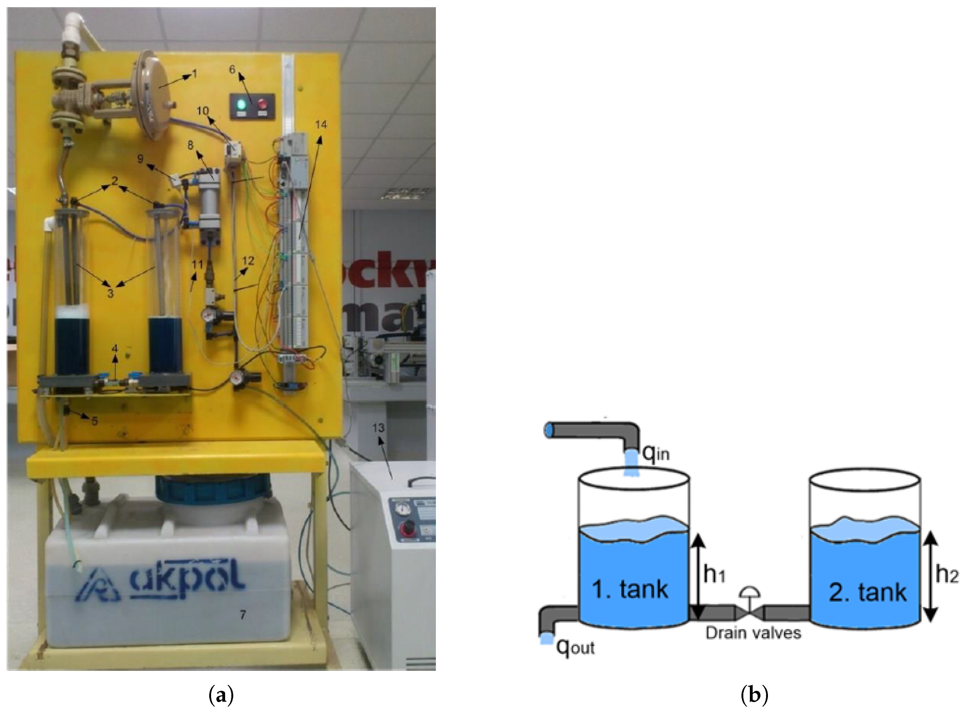
In this paper, a novel approach to the robustness-based autotuner is proposed. Unlike the initial autotuner, which relied on relay and sine tests to determine fundamental parameters, our approach provides a fully automated calculation for these parameters based solely on the time-domain response test. This eliminates the need for additional calculations from the relay and sine tests. To achieve this, the method automatically estimates these values using first-order plus dead time (FOPDT) models. To begin, five diverse step response methods are introduced to ascertain the model parameters in the approach. Second, three alternative estimation methods for the critical frequency of the system are proposed through (i) solving a nonlinear equation, (ii) employing a linear approximation, and (iii) using a power regression. These methods offer flexibility and options for estimating the fundamental parameters. Lastly, the model parameters are then employed to calculate the system frequency response and its derivative at the critical frequency. The subsequent design steps remain unchanged from the initial autotuner. The simulation studies focus on the comparison between the proposed approach and the initial robustness-based autotuning method using two types of overdamped systems. Furthermore, the impact of the step response methods and the proposed estimation methods within the novel approach on system response and control signal is investigated. The designed controllers, utilizing the new approach to the initial autotuner, are implemented on a two-tank liquid-level system. The experimental outcomes align with the simulation results, providing confirmation of the validity and compatibility of the findings.

Existing autotuning methods often rely on relay or sine tests, which are time-consuming, experimentally intensive, and computationally burdensome in industrial settings. Furthermore, while many approaches aim to improve robustness or efficiency, few offer a comprehensive framework that integrates model parameter estimation, critical frequency determination, and robust controller design in a unified process. This gap highlights the need for methods that streamline these steps while ensuring performance and robustness across varying system dynamics. The main contributions of this paper are as follows: (i) A novel approach based on time domain response to the initial autotuner is presented for overdamped systems, (ii) this approach offers a fully automated calculation for fundamental design parameters by eliminating the additional computational burden required by the initial autotuner, (iii) in this approach, three estimation methods for the critical frequency are derived using FOPDT models, and the corresponding algorithms are clearly given, (iii) the effect of the proposed estimation methods in the approach as well as step response methods on system response and control signal are shown in the simulation studies and (iv) PID controllers designed using new approach are applied on a real-time system and perform well as in the initial autotuner.

This paper is organized as follows: the principle of the initial autotuner is discussed in Section 2. Section 3 presents the new approach. The simulation studies are carried out to show the performance of the proposed approach and the effect of proposed estimation methods as well as step response methods on system response in Section 4. Section 5 presents a real-time application of PID controllers designed using the new approach. Section 6 gives some discussions and future studies.

2. The Initial Robustness Based Autotuner

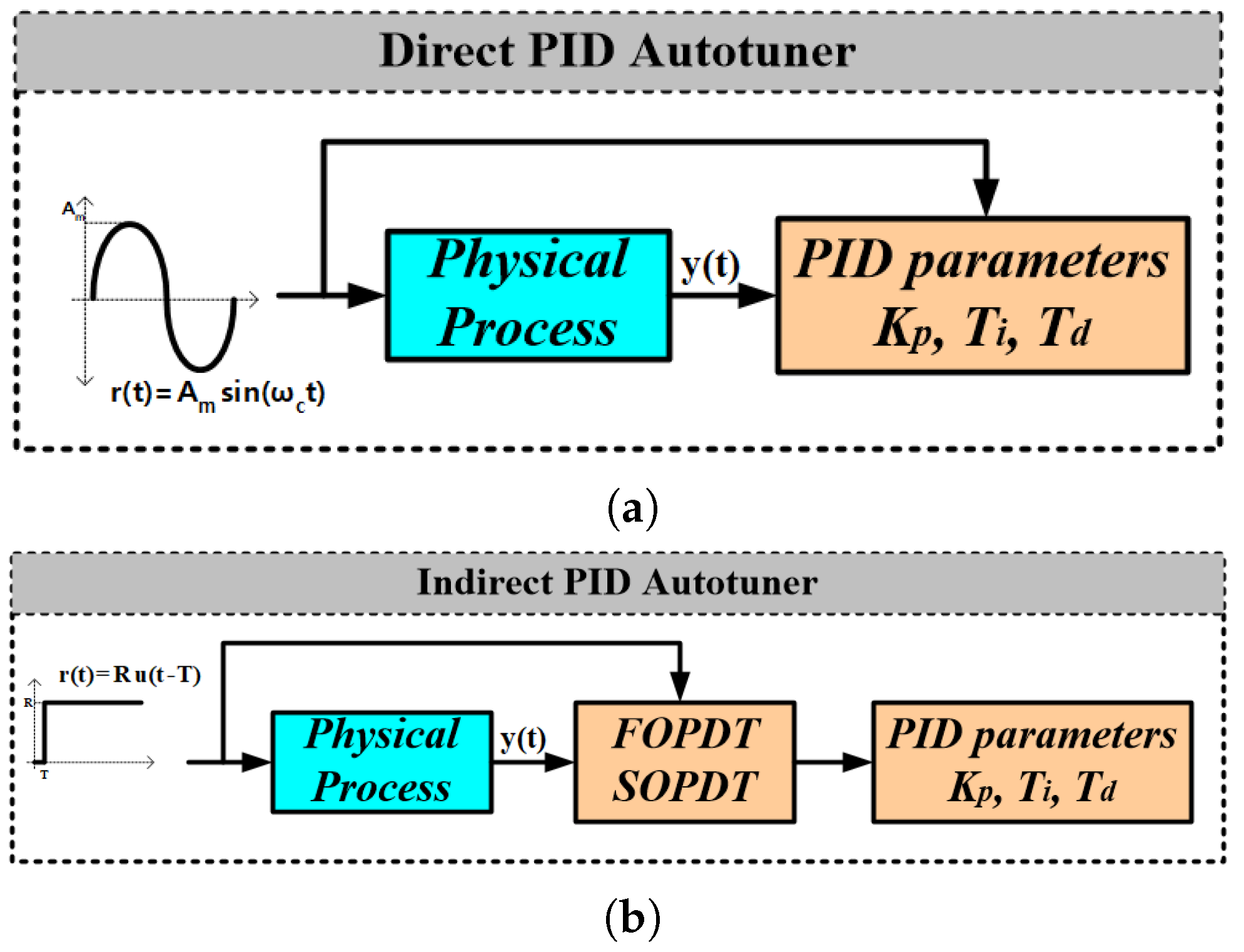
Autotuning methods are divided into two types: Indirect and Direct methods. Indirect methods require the system model to be found with the help of the step response of the system, while direct methods use the system frequency response. The block diagram of these two methods is given in Figure 1. The robust autotuner revisited here is one of the direct PID autotuning methods based on gain margin (GM) and phase margin (PM) specifications. In this method, a quarter-circle, referred to as the ‘forbidden region’, is drawn on the Nyquist plane using these two specifications. The forbidden region is shown in Figure 2 with a red quarter circle. Each point on the forbidden region border can be defined using the radius R and angle $\alpha$. The robust PID controller is then designed to minimize the following measures:

$$\underset{\alpha }{min}\left|\left|{\displaystyle \frac{d{\Im }_b}{d{\Re }_b}}{{|}_{\alpha }-{\displaystyle \frac{d{\Im }_L}{d{\Re }_L}}|}_{\omega ={\omega }_c}\right|\right|,0\le \alpha \le {\alpha }_{max}$$

(1)

where ${\Re }_b$ and ${\Im }_b$ denote the real and imaginary parts of the forbidden region border; ${\Re }_L$ and ${\Im }_L$ represent the real and imaginary parts of the open loop frequency response, which is given in Figure 2 with black curve. Therefore, ${\displaystyle \frac{d{\Im }_b}{d{\Re }_b}}{|}_{\alpha }$ denotes the slope of the forbidden region border in a point with the angle $\alpha$, and is calculated as the selected maximum value of $\alpha$, i.e., ${\alpha }_{max}$. Moreover, ${\displaystyle \frac{d{\Im }_L}{d{\Re }_L}}{|}_{\omega ={\omega }_c}$ is the slope of open-loop frequency response at the critical frequency ${\omega }_c$ of the unknown process $P\left(s\right)$. The critical frequency is described as

$$\angle P\left(j{\omega }_c\right)=-\pi$$

(2)

This method necessitates two tests: (i) a relay test illustrated in Figure 3a is used to estimate the critical frequency, and (ii) a sine test illustrated in Figure 3b to calculate the process frequency response and frequency response slope at the critical frequency [29]. These two tests additionally require further calculations. For instance, the system’s output signal from the relay test contains multiple frequencies as a result of nonlinearity. To determine the dominant frequency, the Fast Fourier Transform (FFT) of the output signal must be applied. After identifying the dominant frequency, during the sine test, a sinusoidal input signal $r\left(t\right)$ is applied to the physical process, producing an output signal $y\left(t\right)$. To compute the phase slope, an additional signal $y^{\prime }\left(t\right)$, representing the derivative of the output, is obtained through a filtering operation. This derivative is derived as $y^{\prime }\left(t\right)=x\left(t\right)-ty\left(t\right)$, where $x\left(t\right)$ is processed from $y\left(t\right)$ using a specific filter, $2s/(s^2+{\omega }_c^2)$. The magnitude and phase are calculated from the amplitude ratio and time shift between the input and output signals, while the phase slope is computed from the processed data. The proposed methodology eliminates the need for additional calculations from the relay and sine tests.

The section is structured as follows: Section 2.1 defines the forbidden region on the Nyquist plane, detailing the calculation of its border slope using gain and phase margin specifications. Section 2.2 explains the determination of the open-loop frequency response slope at the critical frequency, incorporating process frequency components from relay and sine tests.

2.1. The Forbidden Region Border Slope Determination

The following relation defines any points S on the forbidden region border shown in Figure 2:

$$S=-C+Rcos\alpha -jRsin\alpha$$

(3)

where C and R represents the circle center and the circle radius, respectively. One of the two thick points in Figure 2 is determined by relation ${(C-1/GM)}^2=R^2$, and the other is determined by relation ${(-cosPM+C)}^2+{(-sinPM)}^2=R^2$. This leads to the equality $C^2-2CcosPM+1=C^2-2C/GM+1/G{M}^2$. From this, the values of the circle center C and circle radius R can be found as described in [29]:

$$C={\displaystyle \frac{G{M}^2-1}{2GM\left(GMcosPM-1\right)}},R=C-{\displaystyle \frac{1}{GM}}$$

(4)

In this study, phase and gain margins are taken as ${45}^{\circ }$ and 2, respectively [29]. The slope of any points S on the forbidden region border can be found using the following formula:

$${\displaystyle \frac{d{\Im }_b}{d{\Re }_b}}{|}_{\alpha }=cot\alpha$$

(5)

where ${\Re }_b$ and ${\Im }_b$ denote the real and imaginary parts of the forbidden region border, respectively. This slope corresponds to the slope of the blue line in Figure 2.

2.2. The Open Loop Frequency Response Slope Determination

The open loop frequency response $L\left(j\omega \right)$ is described as follows:

$$L\left(j\omega \right)=P\left(j\omega \right)C\left(j\omega \right)$$

(6)

where $P\left(j\omega \right)$ and $C\left(j\omega \right)$ denote the frequency responses of process and PID controller, respectively.

The derivative of the open loop frequency response $L\left(j\omega \right)$ at the critical frequency ${\omega }_c$ is calculated using the following formula:

$${\displaystyle \frac{dL\left(j\omega \right)}{d\omega }}{|}_{\omega ={\omega }_c}=C\left(j{\omega }_c\right){\displaystyle \frac{dP\left(j\omega \right)}{d\omega }}{{|}_{\omega ={\omega }_c}+P\left(j{\omega }_c\right){\displaystyle \frac{dC\left(j\omega \right)}{d\omega }}|}_{\omega ={\omega }_c}$$

(7)

Here, the process frequency components, i.e., $P\left(j{\omega }_c\right)$ and ${\displaystyle \frac{dP\left(j\omega \right)}{d\omega }}{|}_{\omega ={\omega }_c}$ are obtained utilizing the sine test shown in Figure 3b. For the controller frequency components, i.e., $C\left(j{\omega }_c\right)$ and ${\displaystyle \frac{dC\left(j\omega \right)}{d\omega }}{|}_{\omega ={\omega }_c}$ the transfer function structure of PID controller can be given as

$$C\left(s\right)=K_p\left(1+{\displaystyle \frac{1}{T_{i}s}}+T_{d}s\right)$$

(8)

where $K_p$ is the gain of the controller. In the method, it is assumed that the integral time constant $T_i$ is equal to four times the derivative time constant $T_d$. This is a commonly used choice to simplify the tuning procedure; it assumes two identical real zeros in the PID controller [29]. The frequency response of the PID controller is then determined as follows:

$$C\left(j\omega \right)=K_p+j{K}_p\left({\displaystyle \frac{T_i}{4}}\omega -{\displaystyle \frac{1}{T_i\omega }}\right)$$

(9)

On the other hand, since the frequency response values of open loop transfer function $L\left(j{\omega }_c\right)$ and process $P\left(j{\omega }_c\right)$ at ${\omega }_c$ are known, the frequency response value of PID controller $C\left(j{\omega }_c\right)$ at ${\omega }_c$ could easily be calculated employing the following equation:

$$C\left(j{\omega }_c\right)={\displaystyle \frac{L\left(j{\omega }_c\right)}{P\left(j{\omega }_c\right)}}$$

(10)

Note that $L\left(j{\omega }_c\right)$ is equal to a point on the forbidden region border. Finally, the PID controller parameters in (9), i.e., $K_p$ and $T_i$ are found using the numerical value of $L\left(j\omega \right)$ in (10).

The derivative of the frequency response of the PID controller with respect to frequency is found as

$${\displaystyle \frac{dC\left(s\right)}{ds}}=K_p\left({\displaystyle \frac{T_i}{4}}-{\displaystyle \frac{1}{T_i{s}^2}}\right)\Rightarrow {\displaystyle \frac{dC\left(j\omega \right)}{d\omega }}=j{K}_p\left({\displaystyle \frac{T_i}{4}}+{\displaystyle \frac{1}{T_i{\omega }^2}}\right)$$

(11)

Then, the numerical value of ${\displaystyle \frac{dC\left(j\omega \right)}{d\omega }}{|}_{\omega ={\omega }_c}$ is obtained by replacing $\omega$ with ${\omega }_c$ in (11). After finding all the unknown variables in (7), ${\displaystyle \frac{dL\left(j\omega \right)}{d\omega }}{|}_{\omega ={\omega }_c}$ is separated into real ${\Re }_L\left(j\omega \right)$ and imaginary ${\Im }_L\left(j\omega \right)$ parts as follows:

$${\displaystyle \frac{dL\left(j\omega \right)}{d\omega }}{|}_{\omega ={\omega }_c}={\displaystyle \frac{d{\Re }_L\left(j\omega \right)}{d\omega }}{{|}_{\omega ={\omega }_c}+{\displaystyle \frac{d{\Im }_L\left(j\omega \right)}{d\omega }}|}_{\omega ={\omega }_c}$$

(12)

Finally, the open loop frequency slope value is determined as the ratio of the imaginary and real parts, ${\displaystyle \frac{d{\Im }_L}{d{\Re }_L}}{|}_{\omega ={\omega }_c}$

3. The Proposed Strategy

The new strategy relies on only the time domain response test instead of two experiments in the initial robustness-based autotuner. Moreover, the new strategy eliminates the need for additional calculations required by these two experiments, such as FFT computation, filtering, and time-domain convolution. Instead, it proposes a fully automated calculation based solely on the time-domain response test. This strategy concentrates on the processes having an S-shaped time domain response which could simply be described by the FOPDT model. The transfer function of the FOPDT model can be given as

$$G\left(s\right)={\displaystyle \frac{K}{Ts+1}}{e}^{-Ls}$$

(13)

Here, $T,K$ and L are the time constant, gain and time delay of the model, respectively. These parameters are discovered using a step response method in the new strategy. Both the critical frequency and the frequency components of the process at this frequency are estimated by employing the model parameters. The remaining steps are identical to the initial autotuner.

The steps of the initial robustness-based autotuner and the new strategy that we propose in this paper are summarized in Figure 4. It should be noted that the initial autotuner requires two tests, i.e., the relay and sine tests given in Figure 3, whereas the new strategy relies just on the process step response test.

This section is organized as follows: The proposed strategy begins with FOPDT model parameter determination in Section 3.1, where model parameters such as time constant, gain, and delay time are derived using step response methods. These include (i) Smith (SmM), (ii) Sundaresan–Krishnaswamy (SKM), (iii) Ziegler–Nichols (ZNM), (iv) Nishikawa (NiM), and (v) Optimization (Opt). Next, the strategy moves to Critical Frequency Estimation in Section 3.2, which is achieved through one of three methods: (a) solving a nonlinear equation for accurate determination, (b) employing a linear approximation for simplicity, or (c) applying a power regression for data-driven estimation. Once the critical frequency is determined, the strategy proceeds to Frequency Component Estimation in Section 3.2, calculating the process frequency response and its derivative at this frequency. Finally, the PID Controller Design step involves using the estimated parameters to compute the proportional gain, integral time, and derivative time for the controller.

3.1. The First Order Plus Dead Time (FOPDT) Model Parameters Determination

There exist various step response methods to find FOPDT model parameters: Smith step response Method (SmM) [2], Sundaresan–Krishnaswamy step response Method (SKM) [3], Ziegler–Nichols step response Method (ZNM) [1], Nishikawa step response Method (NiM) [4], etc. Firstly, Smith’s and Sundaresan–Krishnaswamy step response methods employ the normalized response ${\displaystyle \frac{y\left(t\right)}{KR}}$ by applying a step function $R\left(s\right)={\displaystyle \frac{R}{s}}$.

The gain is found by using the following formula:

$$K={\displaystyle \frac{y\left(t_f\right)-y\left(t_0\right)}{R}}$$

(14)

where $y\left(t_f\right)$ and $y\left(t_0\right)$ denote the final and initial values of the output signal, respectively. In SmM, two different times are specified such that the normalized response reaches $28.3\%$ at $t_1$ and $63.2\%$ at $t_2$ of its final value, which is illustrated in Figure 5a. In SKM, two different times are again specified such that the normalized response reaches $35.3\%$ at $t_1$ and $85.3\%$ at $t_2$ of its final value, which is depicted in Figure 5b. FOPDT model parameters are found using (15a) and (15b) via two different samples in SmM and SKM, respectively.

$$\begin{array}{cc}\hfill T& =1.5(t_2-t_1),L=(t_2-T)\hfill \end{array}$$

(15a)

$$\begin{array}{cc}\hfill T& =0.67(t_2-t_1),L=(1.3t_1-0.29t_2)\hfill \end{array}$$

(15b)

Secondly, a line at an inflection point of the step response is drawn to obtain the model parameters in ZNM. Figure 6a illustrates how to find model parameters using this line. The difference between the time instants $t_1$ and $t_2$ when the line through the inflection point intersects the vertical lines $y=y\left(t_0\right)$ and $y=y\left(t_f\right)$, respectively, gives time constant value T of the model. On the other hand, the time delay L of the model is found via the time difference $t_1-t_0$.

Thirdly, green and yellow colored areas shown in Figure 6b must be calculated to find model parameters via NiM. $t_1$ must be found using (16a) so that the area $A_1$ can be calculated. Then, FOPDT model parameters are found using (16b) in NiM.

$$\begin{array}{cc}\hfill t_1& ={\displaystyle \frac{A_0}{y\left(t_f\right)-y\left(t_0\right)}}+t_0\hfill \end{array}$$

(16a)

$$\begin{array}{cc}\hfill T& ={\displaystyle \frac{A_1}{0.368(y\left(t_f\right)-y\left(t_0\right))}},L=(t_1-t_0)-T\hfill \end{array}$$

(16b)

Finally, the model parameters can be found by minimizing the following performance index via an optimization algorithm, e.g., a genetic algorithm with a cost function defined as follows:

$$\underset{K,T,L}{min}\left|\right|y_P\left(t\right)-y_G\left(t\right)\left|\right|$$

(17)

where $y_P\left(t\right)$ and $y_G\left(t\right)$ denote real-time system and model responses, respectively. This step response method is referred to as Opt in the study.

3.2. Estimation of the Critical Frequency

In the subsection, three estimation methods are proposed for the critical frequency of the system: Nonlinearity-based, Linear approximation-based, and Power regression-based estimation methods.

3.2.1. Nonlinearity-Based Estimation Method

The analytical expression of the frequency response of the model in (13) is obtained as follows:

$$G\left(j\omega \right)={\displaystyle \frac{K}{1+j\omega T}}{e}^{-j\omega L}$$

(18)

The magnitude and phase responses of the analytical expression are as follows:

$$\left|G\left(j\omega \right)\right|={\displaystyle \frac{K}{\sqrt{1+{\left(\omega T\right)}^2}}},\angle G\left(j\omega \right)=-arctan\left(\omega T\right)-\omega L$$

(19)

For the critical frequency estimation ${\omega }_{c\_est}$, the phase response must be equal to $-(2k+1)\pi ,$ $k=0,1,\dots$. Therefore, the following nonlinear equation has to be solved:

$$\angle G\left(j{\omega }_{c\_est}\right)=-(2k+1)\pi ,k=0,1,\dots$$

(20)

Using the phase response in (19), the following equation is obtained:

$$-arctan\left({\omega }_{c\_est}T\right)-{\omega }_{c\_est}L=-(2k+1)\pi ,k=0,1,\dots$$

(21)

This equation might be reorganized as

$${\omega }_{c\_est}=g\left({\omega }_{c\_est}\right)={\displaystyle \frac{-arctan\left({\omega }_{c\_est}T\right)+(2k+1)\pi }{L}},k=0,1,\dots$$

(22)

The function $arctan{\omega }_{c\_est}T$ is defined within the range $\left(0,{\displaystyle \frac{\pi }{2}}\right)$. Specifically, when $arctan\left({\omega }_{c\_est}T\right)$ = $0$, the corresponding value of ${\omega }_{c\_est}$ is given by ${\omega }_{c\_est}={\displaystyle \frac{2k\pi +\pi }{L}}$, which represents the upper bound. Conversely, when $arctan\left({\omega }_{c\_est}T\right)={\displaystyle \frac{\pi }{2}}$, the value of ${\omega }_{c\_est}$ becomes ${\omega }_{c\_est}={\displaystyle \frac{2k\pi +\frac{\pi }{2}}{L}}$, representing the lower bound. Therefore, the solutions of the nonlinear equation are located within the following intervals:

$${\omega }_{c\_est}\in \left({\displaystyle \frac{2k\pi +\frac{\pi }{2}}{L}},{\displaystyle \frac{2k\pi +\pi }{L}}\right),k=0,1,\dots$$

(23)

For example, consider that the model parameters are $K=1,T=1,L=2$. The Nyquist diagram of the model can be illustrated in Figure 7a. Moreover, Figure 7b depicts the solutions inside the first three intervals, i.e., ${\omega }_{c\_est}\in ({\displaystyle \frac{0.5\pi }{L}},{\displaystyle \frac{\pi }{L}})\cup ({\displaystyle \frac{2.5\pi }{L}},{\displaystyle \frac{3\pi }{L}})\cup ({\displaystyle \frac{4.5\pi }{L}},{\displaystyle \frac{5\pi }{L}})$. These solutions are consistent with the results obtained by Nyquist diagram.

Among several solutions of the nonlinear equation, it is necessary to determine the frequency at which the greatest magnitude is located. It corresponds to the smallest frequency because the magnitude response in (19) diminishes as $\omega$ increases. For $k=0$, the nonlinear equation becomes the following:

$${\omega }_{c\_est}=g\left({\omega }_{c\_est}\right)={\displaystyle \frac{-arctan{\omega }_{c\_est}T+\pi }{L}}$$

(24)

and the solution ${\omega }_{c\_est}$ is located in the interval $(\pi /2L,\pi /L)$. The nonlinear equation might be solved employing fixed point iteration [32]. In this study, we propose two estimation methods to simplify it: (I) Linear approximation-based, and (ii) Power Regression-based estimation methods, described hereafter.

3.2.2. Linear Approximation-Based Estimation Method

Another method can be that a linear function $g_a\left({\omega }_{c\_est}\right)$ in the mentioned interval is approximated for the function $g\left({\omega }_{c\_est}\right)$. The start point of the function $g\left({\omega }_{c\_est}\right)$ is $({\displaystyle \frac{\pi }{2L}},{\displaystyle \frac{-arctan\frac{\pi T}{2L}+\pi }{L}})$ and the endpoint of the function $g\left({\omega }_{c\_est}\right)$ is $({\displaystyle \frac{\pi }{L}},{\displaystyle \frac{-arctan\frac{\pi T}{L}+\pi }{L}})$ Then, the slope of the linear function for $g\left({\omega }_{c\_est}\right)$ can be calculated as

$$m={\displaystyle \frac{-arctan\frac{\pi T}{L}+arctan\frac{\pi T}{2L}}{\frac{\pi }{2}}}$$

(25)

The linear approximation for the function $g\left({\omega }_{c\_est}\right)$ is obtained as

$$g_a\left({\omega }_{c\_est}\right)=m\left({\omega }_c-{\displaystyle \frac{\pi }{L}}\right)+{\displaystyle \frac{-arctan\frac{\pi T}{L}+\pi }{L}}$$

(26)

Finally, the approximated critical frequency can be found using the following formula:

$${\omega }_{c\_est}=g_a\left({\omega }_{c\_est}\right)\Rightarrow {\omega }_{c\_est}={\displaystyle \frac{\pi }{L}}-{\displaystyle \frac{arctan\frac{\pi T}{L}}{(1-m)L}}$$

(27)

3.2.3. Power Regression-Based Estimation Method

The third method uses regression analysis. For this aim, the critical frequency values are found for different $T\in (0.1,15)$ and $L\in (0.1,10)$. The surface shown in Figure 8a illustrates these frequency values. It can be observed from this figure that the test frequency values for FOPDT models are more dependent on time delay than time constant (or settling time). If the effect of time constant is ignored, the following power function can be derived in terms of time delay using MATLAB Curve Fitting Toolbox [33]:

$${\omega }_{c\_est}={\displaystyle \frac{1.785}{L^{0.985}}}$$

(28)

Figure 8b illustrates the derived function in (28) alongside the test frequency values. The color of the points in the figure varies based on the time constant.

3.3. The Frequency Components Estimation at the Critical Frequency

After the estimation of the critical frequency ${\omega }_{c\_est}$, the following frequency response of the system model is used to estimate the process frequency response at the critical frequency

$$P_{est}\left(j{\omega }_c\right)\approx G\left(j{\omega }_{c\_est}\right)=-{\displaystyle \frac{K}{\sqrt{1+{\left({\omega }_{c\_est}T\right)}^2}}}$$

(29)

Firstly, we need to take the derivative of the system model with respect to s so as to calculate the derivative of the frequency response with respect to frequency. Secondly, when s is replaced with $j\omega$, the derivative of the frequency response with respect to frequency is calculated using the following formula:

$${\displaystyle \frac{d{P}_{est}\left(j\omega \right)}{d\omega }}{{|}_{\omega ={\omega }_c}\approx {\displaystyle \frac{dG\left(j\omega \right)}{d\omega }}|}_{\omega ={\omega }_{c\_est}}=-j{\displaystyle \frac{K{e}^{-j{\omega }_{c\_est}L}\left(j{\omega }_{c\_est}TL+T+L\right)}{{(j{\omega }_{c\_est}T+1)}^2}}$$

(30)

After estimating the critical frequency and its corresponding frequency components, the steps outlined in Figure 4 should be followed to determine the PID controller parameters. These steps are detailed in Algorithms A1 and A2 in Appendix A, summarizing the procedures of the initial robustness-based autotuner and its new strategy, respectively.

When a PID controller is applied in practice, incorporating a filter into the derivative term, i.e., ${\displaystyle \frac{T_{d}s}{T_{f}s+1}}$ is often essential. In this study, the filter is adjusted to ensure that the added artificial pole does not affect the system’s dominant dynamics. For both simulation and real-time experiments, the time constant $T_f$ of the filter is set to $T_d/100$.

4. Simulation Studies

In this section, we select three types of overdamped systems—specifically, higher-order processes with current poles, those with real right-half plane zero, and those with multiple zeros—to validate the effectiveness of our proposed strategy.

4.1. Simulation I: A Class of Higher Order Processes with Concurrent Poles

The following overdamped system is considered:

$$G\left(s\right)={\displaystyle \frac{1}{{(s+1)}^9}}$$

(31)

When the relay test is applied to the system, the critical frequency of the system is very close to the actual critical frequency, 0.3640 rad/s. On the other hand, when the sine signal with the critical frequency is applied to the system, the frequency response and its derivative are calculated as −0.5713 and $4.8317e^{j1.2217}$, respectively.

When the mentioned five step response methods, i.e., SmM, SKM, ZNM, NiM and Opt, are employed, the system model parameters are obtained as $T=3.91,L=5.79$; $T=3.01,L=6.38$; $T=7.16,L=5.08$; $T=3.22,L=5.78$ and $T=3.56,L=5.78$, respectively. For each model parameter, the critical frequency values are estimated using three methods, i.e., Nonlinear, Analytical and Regression. The estimated critical frequency values are given in

Table 1. Estimated ${\omega }_c$ values for the higher order processes with concurrent poles.

	Nonlinear	Analytical	Regression
SmM	0.3748 (2.98%)	0.3801 (4.43%)	0.3165 (13.03%)
SKM	0.3627 (0.35%)	0.3667 (0.74%)	0.2879 (20.91%)
ZNM	0.3787 (4.04%)	0.3831 (5.26%)	0.3600 (01.10%)
NiM	0.3885 (6.75%)	0.3935 (8.10%)	0.3172 (12.85%)
Opt	0.3814 (4.80%)	0.3866 (6.22%)	0.3169 (12.93%)

. It can be easily seen that the best estimation for the critical frequency is made by SKM. Moreover, nonlinear and analytical methods to estimate the critical frequency for all step response methods give closer results to each other.

The nonlinearity-based estimation method is initially employed to estimate the critical frequency to assess the impact of modeling on the system response. Following this, the PID parameters are computed using Algorithm A2. These values are shown in

Table 2. PID parameter values using nonlinear method for the higher order processes with concurrent poles.

	${\mathit{K}}_{\mathit{p}}$	${\mathit{T}}_{\mathit{i}}$	${\mathit{T}}_{\mathit{d}}$
The initial autotuner	0.8888	7.2518	1.8130
The autotuner using SmM	0.8938	6.5348	1.6337
The autotuner using SKM	0.7434	6.3905	1.5976
The autotuner using ZNM	1.4738	7.1899	1.7975
The autotuner using NiM	0.8063	6.1673	1.5418
The autotuner using Opt	0.8491	6.3513	1.5878

. The corresponding system responses and control signals are illustrated in Figure 9a and Figure 9b, respectively. The autotuners using the four step response methods other than the Ziegler–Nichols method have satisfactory results. However, the least overshoot and the faster settling time are obtained using SKM. The higher proportional gain in a PID controller enhances the system’s response speed; however, it frequently induces overshoot, as the system becomes prone to excessively aggressive reactions to errors.

The PID parameters, as detailed in

Table 3. PID parameter values based on SKM for the higher-order processes with concurrent poles.

	${\mathit{K}}_{\mathit{p}}$	${\mathit{T}}_{\mathit{i}}$	${\mathit{T}}_{\mathit{d}}$
Nonlinear	0.7434	6.3905	1.5976
Analytical	0.7441	6.5216	1.6304
Regression	0.6927	5.3421	1.3355

, are calculated to assess the impact of the proposed critical frequency estimation methods on the system response. In this case, SKM is selected as the step response method. The corresponding system responses and control signals are illustrated in Figure 10a and Figure 10b, respectively. The autotuners using the three proposed estimation methods have satisfactory results. Especially, the nonlinear and analytical methods give very close results to each other and they possess the least overshoot and faster settling time.

4.2. Simulation II: A Class of Higher Order Processes with the Real Half Plane Zero

The following transfer function is considered a higher process with the real half-plane zero:

$$G_2\left(s\right)={\displaystyle \frac{1-s}{{(s+1)}^3}}$$

(32)

Also, the critical frequency of the system is very close to the actual critical frequency, 1 rad/s. On the other hand, when the sine signal with the critical frequency is applied to the system, the frequency response and its derivative are calculated as −0.5000 and $1.1180e^{j1.1071}$, respectively.

When the mentioned five step response methods, i.e., SmM, SKM, ZNM, NiM and Opt, are employed, the system model parameters are obtained as $T=1.96,L=2.12$; $T=1.69,L=2.30$; $T=3.24,L=1.85$; $T=1.59,L=2.41$ and $T=1.86,L=2.11$, respectively. For each model parameter, the critical frequency values are estimated using three methods, i.e., Nonlinear, Analytical and Regression. The estimated critical frequency values are given in

Table 4. Estimated ${\omega }_c$ values for the higher order processes with the real half plane zero.

	Nonlinear	Analytical	Regression
SmM	0.9707 (2.93%)	0.9848 (1.52%)	0.8529 (14.71%)
SKM	0.9307 (6.93%)	0.9441 (5.59%)	0.7868 (21.32%)
ZNM	1.0077 (0.77%)	1.0175 (1.75%)	0.9718 (2.82%)
NiM	0.9046 (9.54%)	0.9172 (8.28%)	0.7514 (24.86%)
Opt	0.9816 (1.84%)	0.9959 (0.41%)	0.8554 (14.46%)

. It can be easily seen that the best estimation for the critical frequency is made by ZNM and Opt methods. Moreover, nonlinear and analytical methods to estimate the critical frequency for all step response methods give closer results to each other.

As in Simulation I, the nonlinearity-based estimation method is first employed in Simulation II to estimate the critical frequency in order to evaluate the impact of modeling on the system response. Subsequently, the PID parameters are computed using Algorithm A2. These values are shown in

Table 5. PID parameter values using nonlinear method for the higher-order processes with the real half plane zero.

	${\mathit{K}}_{\mathit{p}}$	${\mathit{T}}_{\mathit{i}}$	${\mathit{T}}_{\mathit{d}}$
Initial autotuner	1.0322	2.9465	0.7366
The autotuner using SmM	1.0879	2.6342	0.6585
The autotuner using SKM	0.9392	2.6603	0.6651
The autotuner using ZNM	1.7438	2.7569	0.6892
The autotuner using NiM	0.8842	2.7076	0.6769
The autotuner using Opt	1.0543	2.6051	0.6513

. The corresponding system responses and control signals are illustrated in Figure 11a and Figure 11b, respectively. The autotuners using the four step response methods other than Ziegler–Nichols method have satisfactory results. However, the least overshoot and the faster settling time are obtained using NiM.

The PID parameters, as shown in

Table 6. PID parameter values based on NiM using the higher order processes with the real half plane zero.

	${\mathit{K}}_{\mathit{p}}$	${\mathit{T}}_{\mathit{i}}$	${\mathit{T}}_{\mathit{d}}$
Nonlinear	0.8842	2.7076	0.6769
Analytical	0.8849	2.7429	0.6857
Regression	0.8483	2.3913	0.5978

, are computed to evaluate the impact of the proposed critical frequency estimation methods on the system response. Here, NiM is chosen as the step response method. The corresponding system responses and control signals are illustrated in Figure 12a and Figure 12b, respectively. The autotuners using the three proposed estimation methods have satisfactory results. Especially, the nonlinear and analytical methods give very close results to each other and they possess the least overshoot and faster settling time.

4.3. Simulation III: A Class of Higher Order Processes with Multiple Zeros and Dead Time

The following transfer function is considered as higher processes with multiple zeros, i.e., two real half-plane zeros, and dead time:

$$G_3\left(s\right)={\displaystyle \frac{0.164(s-0.333)(s-0.2)}{{(s+0.25)}^2(s+0.1)}}{e}^{-1.25s}$$

(33)

The critical frequency of the system is very close to the actual critical frequency, 0.1392 rad/s. On the other hand, when the sine signal with the critical frequency is applied to the system, the frequency response and its derivative are calculated as −1.028 and $17.83e^{j1.29}$, respectively.

When the mentioned five step response methods, i.e., SmM, SKM, ZNM, NiM and Opt, are employed, the system model parameters are obtained as $T=12.14,L=15.16$; $T=10.98,L=16.01$; $T=18.83,L=13.86$; $T=10.53,L=16.71$ and $T=11.87,L=15.06$, respectively. For each model parameter, the critical frequency values are estimated using three methods, i.e., Nonlinear, Analytical and Regression. The estimated critical frequency values are given in

Table 7. Estimated ${\omega }_c$ values for the higher order processes with multiple zeros and dead time.

	Nonlinear	Analytical	Regression
SmM	0.1389 (0.0023%)	0.1409 (0.0123%)	0.1226 (0.1191%)
SKM	0.1351 (0.0296%)	0.1370 (0.0158%)	0.1162 (0.1654%)
ZNM	0.1395 (0.0022%)	0.1412 (0.0143%)	0.1339 (0.0380%)
NiM	0.1314 (0.0559%)	0.1332 (0.0429%)	0.1114 (0.1995%)
Opt	0.1404 (0.0087%)	0.1425 (0.0234%)	0.1236 (0.1117%)

. It can be easily seen that the critical frequency estimation results are comparable among all identification methods. Moreover, nonlinear and analytical methods to estimate the critical frequency for all step response methods give closer results to each other.

As in Simulation II, the nonlinearity-based estimation method is first employed in Simulation III to estimate the critical frequency in order to evaluate the impact of modeling on the system response. Subsequently, the PID parameters are computed using Algorithm A2. These values are shown in

Table 8. PID parameter values using nonlinear method for the higher order process with multiple zeros and dead time.

	${\mathit{K}}_{\mathit{p}}$	${\mathit{T}}_{\mathit{i}}$	${\mathit{T}}_{\mathit{d}}$
Initial autotuner	0.4909	17.9789	4.4947
The autotuner using SmM	0.5661	18.0229	4.5057
The autotuner using SKM	0.5157	18.1329	4.5332
The autotuner using ZNM	0.8182	19.3177	4.8294
The autotuner using NiM	0.4918	18.4350	4.6087
The autotuner using Opt	0.5613	17.8270	4.4568

. The corresponding system responses and control signals are illustrated in Figure 13a and Figure 13b, respectively. The autotuners using the four step response methods other than the Ziegler–Nichols method have satisfactory results. However, the least overshoot and the faster settling time are obtained using NiM.

The PID parameters, as shown in

Table 9. PID parameter values based on NiM using the higher order processes with multiple zeros and dead time.

	${\mathit{K}}_{\mathit{p}}$	${\mathit{T}}_{\mathit{i}}$	${\mathit{T}}_{\mathit{d}}$
Nonlinear	0.4918	18.4350	4.6087
Analytical	0.4922	18.6703	4.6676
Regression	0.4733	16.3822	4.0955

, are computed to evaluate the impact of the proposed critical frequency estimation methods on the system response. Here, NiM is chosen as the step response method. The corresponding system responses and control signals are illustrated in Figure 14a and Figure 14b, respectively. The autotuners using the three proposed estimation methods have satisfactory results. Especially, the nonlinear and analytical methods give very close results to each other and they possess the least overshoot and faster settling time.

For robustness analysis, PID parameters are selected using the NiM method for step response tuning and a nonlinear method for estimating critical gain. To evaluate robustness, the system gain and time delay were altered by ±10%. Figure 15 displays the system responses under these variations. It is evident that the controller demonstrates robustness against changes in both gain and dead time of the process in (33). Notably, the system is more resilient to time delay variations compared to gain changes.

5. An Experimental Study on Two-Tank Liquid-Level System

In this section, the controllers designed using the proposed strategy are applied to the real-time two-tank liquid-level system to validate practically the effectiveness of our proposed strategy. Moreover, they are compared with initial autotuner.

5.1. Description of Two-Tank Liquid-Level System

The general view of the two-tank liquid-level control system is given in Figure 16a. The names of elements in the system in Figure 16 are depicted in

Table 10. The names of elements in two tank liquid level system.

No	Element Name	No	Element Name
1	Proportional valve	8	Pressure sensor (1. tank)
2	Pipes for pressure	9	Pressure sensor (2. tank)
3	Tanks	10	Electropneumatic regulator
4	Transition valves	11	Cable for level data
5	Drain valves	12	Cable for flow rate data
6	Start/Stop buttons	13	Compressor
7	Depot	14	Input/Output unit of PLC

. In this system, the water in depot (No 7) is continuously pumped to the liquid inlet by a motor. The liquid flow rate depends on the position of the proportional valve (No 1). The liquid input is carried out only through the first tank (No 3) and liquid flow into the second tank (No 3) is provided by means of transition valves (No 4) between the two tanks. The drainage of the water to the depot is realized through drain valves (No 5) on the first tank. Both of the tanks have a diameter of 10 cm and a height of 50 cm.

Electro-pneumatic elements are utilized to set the position of the proportional valve and measure the level of liquids. The compressed air required to be able to operate electro-pneumatic elements is provided by the compressor (No 13). An electro-pneumatic regulator (No 10) sets the position of a proportional valve (No 1) by transforming a current signal between 4 and 20 mA to air pressure between 0.7 and 14 psi. Thus, the amount of fluid flow rate permitted by the proportional valve is electrically adjusted using the cable (No 10).

The liquid levels in the tanks (No 3) are measured using the pressure change in the level sensors immersed in the tanks. Pressure/voltage transducers (No 8 and 9) transform pressure information depending on the level of liquid to voltage signals between 1 and 5 V. Then, using the cable (No 11), these signals are transmitted to the input/output unit of the Programmable Logic Controller (PLC) (No 14) as feedback. Moreover, the start button (No 6) initiates operation by supplying power to the system or activating the control. The stop button (No 6), on the other hand, stops the operation of the system and cuts off the power. Inside the tank, there exist pipes (No 2) connected to pressure sensors. These pipes transmit the pressure of the liquid to the sensors, which detect changes in the liquid level.

Additionally, Figure 13b illustrates a schematic diagram of a two-tank system. In this setup, $h_1$ and $h_2$ represent the water levels (heights) in the first and second tanks, respectively. The flow rate of water entering the system is denoted by $q_{in}$, while $q_{out}$ represents the flow rate exiting the system. The tanks are connected by drain valves, which regulate the flow between them. The primary objective of this model is to establish a mathematical relationship between the input flow rate ($q_{in}$) and the water level ($h_1$) in the first tank.

5.2. PID Controller Design Using Initial Autotuner

Firstly, the relay test shown in Figure 3a is carried out to find the critical frequency of the two tank liquid level system. The data are collected every 10 ms. The output of the system can be seen in Figure 17a. Since the output is not a pure sinusoidal signal, its Fast Fourier Transform illustrated in Figure 17b is found. As can be seen in the figure, the critical frequency of the system is equal to 0.083 Hz (0.5215 rad/s).

Secondly, the sine test shown in Figure 3b is carried out to find the frequency response and its derivative of the two-tank liquid level system. The data are collected every 10 ms. The output and input signals of the system can be seen in Figure 18a. Figure 18b illustrates the zoom of the output signals. Moreover, since the output is not a pure sinusoidal signal due to the system’s nonlinearity, its Fast Fourier Transform, illustrated in Figure 18c, is obtained. The frequency response and its derivative at the critical frequency are calculated as −0.0071 and $0.0141e^{j1.1222}$, respectively.

5.3. PID Controller Design Using the Proposed Strategy

5.3.1. FOPDT Model for Liquid Level System

When the flow rate of 90 cm³/s is applied to the system, the step response of the system is obtained in Figure 19. For all the mentioned step response methods, the system gain is calculated as follows:

$$K={\displaystyle \frac{10.43-2.51}{90-0}}=0.088$$

(34)

Then, the parameters, i.e., L and T of FOPDT are calculated as $T=31.545,L=6.930$; $T=25.960,$$L=10.301$; $T=11.314,L=27.710$; $T=26.563,L=8.310$ and $T=29.195,$$L=7.121$ using the five step response methods, SmM, SKM, ZNM, NiM and Opt, respectively.

5.3.2. PID Controller Design

For each model parameter, the critical frequency values are estimated using three methods, i.e., Nonlinear, Analytical and Regression. Then, for each combination, PID controller parameters are calculated via Algorithm A2. The estimated critical frequency values and PID parameter values are given

Table 11. The estimated critical frequency values and PID parameters values.

	${\mathit{\omega }}_{\mathit{c}}$ (rad/s)	${\mathit{K}}_{\mathit{p}}$	${\mathit{T}}_{\mathit{i}}$	${\mathit{T}}_{\mathit{d}}$	${\mathit{\omega }}_{\mathit{c}}$ (rad/s)	${\mathit{K}}_{\mathit{p}}$	${\mathit{T}}_{\mathit{i}}$	${\mathit{T}}_{\mathit{d}}$	${\mathit{\omega }}_{\mathit{c}}$ (rad/s)	${\mathit{K}}_{\mathit{p}}$	${\mathit{T}}_{\mathit{i}}$	${\mathit{T}}_{\mathit{d}}$
	Nonlinear				Analytical				Regression
SmM	0.2451	45.34	12.36	3.09	0.2457	45.36	12.40	3.10	0.2650	45.34	12.30	3.08
SKM	0.1737	26.63	16.64	4.16	0.1748	26.66	16.73	4.18	0.1795	26.66	16.78	4.19
ZNM	0.0856	7.93	26.77	6.69	0.0864	7.94	26.94	6.73	0.0677	7.34	21.81	5.45
NiM	0.2103	32.84	14.00	3.50	0.2113	32.87	14.07	3.52	0.2217	32.88	14.15	3.56
Opt	0.2404	41.17	12.48	3.12	0.2412	41.20	12.52	3.13	0.2581	41.19	12.59	3.15

. It can be easily seen that the best estimation for the real critical frequency is made by the SmM method. Moreover, nonlinear and analytical methods to estimate the critical frequency for all identification methods give closer results to each other.

To be able to observe the effect of modeling on the system response, the nonlinear method is first selected for the critical frequency estimation, and then PID parameters are calculated using Algorithm A2. These values are shown in Table 11. The corresponding system responses and control signals are illustrated in Figure 20a and Figure 20b, respectively. The  autotuners using the four identification methods other than the Ziegler–Nichols method have satisfactory results. However, the least overshoot and the faster settling time are obtained using NiM and SKM.

The performance of the designed liquid level control systems is assessed using several criteria, including integral square error (ISE), integral absolute error (IAE), integral time square error (ITSE), and total variation (TV) of the control signal, along with overshoot percentage (OV), settling time (ST), and rise time (RT).

Table 12. Performance measure values of the designed liquid level control systems.

	$\mathit{ISE}(\times {10}^3)$	$\mathit{IAE}(\times {10}^3)$	$\mathit{ITSE}(\times {10}^5)$	$\mathit{TV}(\times {10}^4)$	$\mathit{OV}(\%)$	$\mathit{ST}\left(\mathit{s}\right)$	$\mathit{RT}\left(\mathit{s}\right)$
Initial autotuner	2.604	0.812	3.177	5.646	16.198	59.913	9.577
The autotuner using SmM	1.992	0.592	1.276	3.532	7.821	47.197	30.360
The autotuner using SKM	3.629	0.999	4.772	2.204	10.960	71.024	36.260
The autotuner using ZNM	2.549	0.786	2.951	1.928	26.093	90.067	13.040
The autotuner using NiM	2.963	0.843	3.163	2.974	9.709	57.210	33.970
The autotuner using Opt	2.158	0.634	1.479	3.985	8.355	48.556	32.050

presents the quantitative results for these performance metrics across autotuning methods. Among these metrics, total variation (TV) is a critical indicator as it quantifies the smoothness and variability of the control signal, which directly impacts energy consumption. In this context, the autotuners employing the ZNM and SKM methods demonstrate the lowest TV values, reflecting reduced control effort. However, this reduction in control variability is accompanied by increased ISE and ITSE values, indicating a compromise in error minimization. In contrast, the autotuners utilizing the SmM and Opt methods achieve superior performance in error-based metrics (ISE, IAE, and ITSE), with notable improvements in settling time and overshoot. Nevertheless, these methods exhibit moderately higher TV values, indicating a more dynamic control signal that prioritizes rapid response and precision over smoothness. This analysis highlights a trade-off between control signal smoothness and performance optimization. While the SmM method provides the most balanced solution in terms of error minimization and transient response, the ZNM and SKM methods may be more suitable for applications where minimizing control effort and signal variability is critical.

6. Conclusions

In this paper, a novel approach to an initial frequency response-based autotuner is presented in order to enable the design of robust PID controllers for overdamped systems characterized by an S-shaped step response. In the prior autotuner, which is inherently robust, the critical frequency is established through a relay test, and the process frequency response alongside its derivative at that frequency are acquired via a sine test. In contrast, the new approach, which offers a fully automated calculation for these values, necessitates solely a step test and approximates these values by utilizing FOPDT models obtained based on a step test. Initially, five distinct step response methods are introduced to determine the model parameters. Subsequently, three alternative methods for estimating the critical frequency of the system are put forward by (i) solving a nonlinear equation, (ii) utilizing a linear approximation, and (iii) applying a power regression. Finally, the model parameters are utilized to compute the frequency response and its derivative at the critical frequency. The subsequent design steps remain consistent with the initial frequency-based autotuner. The simulation studies are carried out on two types of overdamped systems, i.e., overdamped systems with concurrent poles and with the real half-plane zero. The controllers developed through the new approach are also put into practice in a two-tank liquid-level system, as an alternative to the initial autotuner. The experimental results align with the outcomes from the simulation, providing confirmation of the accuracy and consistency of the obtained findings. The critical frequency estimation has been observed to yield similar results among various step response methods in both simulation and real-world applications. Furthermore, it has been noted that the nonlinear and analytical methods provide quite similar results when estimating the critical frequency.

The impact of step response methods on PID controller design has been investigated. The robust autotuners employing the four step response methods, excluding the Ziegler–Nichols method, produce satisfactory outcomes. Namely, the autotuner based on SKM or NiM leads to the least overshoot and the fastest settling time. Moreover, the influence of critical frequency estimation methods on PID controller design has also been examined. The autotuners using the three proposed estimation methods yield satisfactory results. Particularly, the nonlinear and analytical methods produce highly similar results, characterized by the least overshoot and the fastest settling time. However, one limitation of the proposed strategy is that it may struggle to provide accurate results when dealing with systems that exhibit high levels of noise or extreme nonlinearities.

References

1. Ziegler, J.G.; Nichols, N.B.; Rochester, N.Y. Optimum settings for automatic controllers. Trans. ASME 1942, 64, 759–764. [Google Scholar] [CrossRef]
2. Smith, C.; Carter, K. Digital Computer Process Control; Intext Educational Pub.: Scranton, PA, USA, 1972. [Google Scholar]
3. Sundaresan, K.; Krishnaswamy, P. Estimation of time delay time constant parameters in time, frequency, and Laplace domains. Can. J. Chem. Eng. 1978, 56, 257–262. [Google Scholar] [CrossRef]
4. Nishikawa, Y.; Sannomiya, N.; Ohta, T.; Tanaka, H. A method for auto-tuning of PID control parameters. Automatica 1984, 20, 321–332. [Google Scholar] [CrossRef]
5. Maxim, A.; De Keyser, R. Estimation of First Order Plus Dead Time and Second Order Plus Dead Time models from noisy step response data. Asian J. Control 2023, 25, 1791–1804. [Google Scholar] [CrossRef]
6. Afram, A.; Janabi-Sharifi, F.; Fung, A.S.; Raahemifar, K. Artificial neural network (ANN) based model predictive control (MPC) and optimization of HVAC systems: A state of the art review and case study of a residential HVAC system. Energy Build. 2017, 141, 96–113. [Google Scholar] [CrossRef]
7. Ionescu, C.; Copot, D. Hands-on MPC tuning for industrial applications. Bull. Pol. Acad. Sciences. Tech. Sci. 2019, 67, 925–945. [Google Scholar] [CrossRef]
8. Rollins Sr, D.K.; Mei, Y. A new feedback predictive control approach for processes with time delay in the manipulated variable. Chem. Eng. Res. Des. 2018, 136, 806–815. [Google Scholar] [CrossRef]
9. Muresan, C.I.; Ionescu, C.M. Generalization of the FOPDT model for identification and control purposes. Processes 2020, 8, 682. [Google Scholar] [CrossRef]
10. Li, H.; Li, R.; Wu, F. A new control performance evaluation based on LQG benchmark for the heating furnace temperature control system. Processes 2020, 8, 1428. [Google Scholar] [CrossRef]
11. Sindhuja, P.P.; Vijayan, V.; Panda, R.C. Control of time-delay systems through modified Smith predictor using sliding mode controller. Int. J. Syst. Sci. 2023, 54, 1961–1986. [Google Scholar] [CrossRef]
12. Xie, S.; Sun, H.; Xie, Y.; Chen, X. Tuning of fuzzy controller with arbitrary triangular input fuzzy sets based on proximal policy optimization for time-delays system. J. Process Control 2023, 129, 103059. [Google Scholar] [CrossRef]
13. Valério, D.; Da Costa, J.S. Tuning of fractional PID controllers with Ziegler–Nichols-type rules. Signal Process. 2006, 86, 2771–2784. [Google Scholar] [CrossRef]
14. Chen, Y.; Bhaskaran, T.; Xue, D. Practical tuning rule development for fractional order proportional and integral controllers. J. Comput. Nonlinear Dyn. 2008, 3, 021403. [Google Scholar] [CrossRef]
15. Li, H.; Luo, Y.; Chen, Y. A fractional order proportional and derivative (FOPD) motion controller: Tuning rule and experiments. IEEE Trans. Control Syst. Technol. 2009, 18, 516–520. [Google Scholar] [CrossRef]
16. Samad, T. A survey on industry impact and challenges thereof. IEEE Control Syst. Mag. 2017, 37, 17–18. [Google Scholar]
17. Åström, K.J.; Hägglund, T. PID Controllers: Theory, Design, and Tuning; ISA—The Instrumentation, Systems and Automation Society: Research Triangle Park, NC, USA, 1995. [Google Scholar]
18. Panagopoulos, H.; Åström, K.J.; Hägglund, T. Design of PID controllers based on constrained optimisation. IEE Proc.-Control Theory Appl. 2002, 149, 32–40. [Google Scholar] [CrossRef]
19. Skogestad, S. Simple analytic rules for model reduction and PID controller tuning. J. Process Control 2003, 13, 291–309. [Google Scholar] [CrossRef]
20. Grimholt, C.; Skogestad, S. Optimal PI and PID control of first-order plus delay processes and evaluation of the original and improved SIMC rules. J. Process Control 2018, 70, 36–46. [Google Scholar] [CrossRef]
21. Wang, Q.; Lu, C.; Pan, W. IMC PID controller tuning for stable and unstable processes with time delay. Chem. Eng. Res. Des. 2016, 105, 120–129. [Google Scholar] [CrossRef]
22. Najafizadegan, H.; Merrikh-Bayat, F.; Jalilvand, A. IMC-PID controller design based on loop shaping via LMI approach. Chem. Eng. Res. Des. 2017, 124, 170–180. [Google Scholar] [CrossRef]
23. Siddiqui, M.A.; Anwar, M.; Laskar, S. Enhanced control of unstable cascade systems using direct synthesis approach. Chem. Eng. Sci. 2021, 232, 116322. [Google Scholar] [CrossRef]
24. So, G.B. A modified 2-DOF control framework and GA based intelligent tuning of PID controllers. Processes 2021, 9, 423. [Google Scholar] [CrossRef]
25. Åström, K.J.; Hägglund, T. Automatic tuning of simple regulators with specifications on phase and amplitude margins. Automatica 1984, 20, 645–651. [Google Scholar] [CrossRef]
26. Tan, K.; Lee, T.; Wang, Q. Enhanced automatic tuning procedure for process control of PI/PID controllers. AIChE J. 1996, 42, 2555–2562. [Google Scholar] [CrossRef]
27. Hang, C.C.; Åström, K.J.; Ho, W.K. Refinements of the Ziegler–Nichols tuning formula. IEE Proc. D (Control. Theory Appl.) 1991, 138, 111–118. [Google Scholar] [CrossRef]
28. Chen, Y.; Hu, C.; Moore, K.L. Relay feedback tuning of robust PID controllers with iso-damping property. In Proceedings of the 42nd IEEE International Conference on Decision and Control (IEEE Cat. No. 03CH37475), Maui, HI, USA, 9–12 December 2003; Volume 3, pp. 2180–2185. [Google Scholar]
29. De Keyser, R.; Muresan, C.; Ionescu, C. Universal direct tuner for loop control in industry. IEEE Access 2019, 7, 81308–81320. [Google Scholar] [CrossRef]
30. De Keyser, R.; Ionescu, C.M.; Muresan, C.I. Comparative evaluation of a novel principle for PID autotuning. In Proceedings of the 2017 11th Asian Control Conference (ASCC), Gold Coast, QLD, Australia, 17–20 December 2017; pp. 1164–1169. [Google Scholar]
31. Copot, C.; Muresan, C.; Ionescu, C.M.; Vanlanduit, S.; De Keyser, R. Calibration of UR10 robot controller through simple auto-tuning approach. Robotics 2018, 7, 35. [Google Scholar] [CrossRef]
32. Mathews, J.H.; Fink, K.D. Numerical Methods Using MATLAB; Pearson Prentice Hall: Upper Saddle River, NJ, USA, 2004; Volume 4. [Google Scholar]
33. The MathWorks Inc. Curve Fitting Toolbox (R2022b). 2022. Available online: https://nl.mathworks.com/products/curvefitting.html (accessed on 1 November 2024).
Figure 1. (a) Direct and (b) indirect autotuning approaches.
Processes 12 02825 g001
Figure 2. The forbidden region (red quarter area), unit circle (green quarter area) and Nyquist diagram of open loop system (black curve).
Processes 12 02825 g002
Figure 3. Block diagrams of (a) relay test and (b) sine test.
Processes 12 02825 g003
Figure 4. The steps of the initial robustness-based autotuner and the proposed strategy. The rectangular blocks show automatically calculated areas. The relay and sine tests in the initial autotuner require further calculations, e.g., FFT calculation, filtering, the convolved with the time signal. The proposed strategy offers a fully automated calculation based solely on the time-domain response test.
Processes 12 02825 g004
Figure 5. An overdamped system characterized by S-shaped response and two corresponding samples for (a) Smith’s and (b) Sundaresan–Krishnaswamy step response methods.
Processes 12 02825 g005
Figure 6. An overdamped system characterized by S-shaped response and samples for (a) Ziegler Nichols and (b) Nishikawa step response methods.
Processes 12 02825 g006
Figure 7. (a) Nyquist diagram and (b) solutions of the nonlinear equation in (21).
Processes 12 02825 g007
Figure 8. (a) The critical frequency values and (b) solutions of the nonlinear equation in (21).
Processes 12 02825 g008
Figure 9. (a) Step responses and (b) control signals of the designed control systems using the higher order processes with concurrent poles.
Processes 12 02825 g009
Figure 10. (a) Step responses and (b) control signals of the designed control systems using the higher order processes with concurrent poles.
Processes 12 02825 g010
Figure 11. (a) Step responses and (b) control signals of the designed control systems using the higher order processes with the real half plane zero.
Processes 12 02825 g011
Figure 12. (a) Step responses and (b) control signals of the designed control systems.
Processes 12 02825 g012
Figure 13. (a) Step responses and (b) control signals of the designed control systems using the higher order process with multiple zeros and dead time.
Processes 12 02825 g013
Figure 14. (a) Step responses and (b) control signals of the designed control systems.
Processes 12 02825 g014
Figure 15. (a) Step responses and (b) control signals the control systems under gain and dead time variations.
Processes 12 02825 g015
Figure 16. (a) General view and (b) schematic diagram of two tank liquid level system.
Processes 12 02825 g016
Figure 17. (a) The output of relay test and (b) Fast Fourier Transform of the output.
Processes 12 02825 g017
Figure 18. (a) input/output signals of the sine test, (b) output signal of the sine test and (c) Fourier transforms of input/output signals.
Processes 12 02825 g018
Figure 19. Step response of the two-tank liquid level system.
Processes 12 02825 g019
Figure 20. (a) Step responses and (b) control signals of the designed liquid level control systems.
Processes 12 02825 g020