Research on Oscillation Suppression Control Method for Contact Scanning Motion

Abstract

Contact scanning sensors play a crucial role in certain detection equipment, enabling the precise identification and detection of structural degradation to effectively mitigate risks. However, these sensors face a challenge: during high-speed scanning, vibrations can occur due to surface unevenness and friction. These vibrations not only compromise the scanning accuracy but also expedite sensor wear and tear. To address this issue, this study introduces a control strategy. By precisely regulating the actuator’s output, we aim to adjust the sensor’s motion, minimizing vibrations and enhancing the detection system’s stability and accuracy. Simulation results demonstrate that this strategy significantly improves scanning quality and reduces vibrations, validating its effectiveness. These findings pave the way for future research and technological applications.

1. Introduction

In current engineering projects, ultrasonic detection technology is renowned for its efficiency and sensitivity, playing a crucial role in key areas such as assessing structural aging, analyzing metal manufacturing processes, and inspecting welding quality. This type of inspection typically relies on contact scanning sensors equipped with ultrasonic technology [1,2,3,4]. However, during high-speed scanning, vibrations may occur in the sensing equipment due to surface irregularities and friction, thereby affecting measurement accuracy. The main reason is that surface unevenness alters the incident angle of ultrasonic waves on the material surface, significantly compromising the accuracy of detection results. Additionally, frequent vibrations reduce the durability of the mechanical structure of the sensing system. To ensure high-precision detection results, operators often have to reduce the scanning speed. Since the vibration amplitudes of different material surfaces vary depending on surface conditions, operators rely on experience and multiple trials to adjust the scanning speed and control vibrations within an acceptable range.

Such vibration suppression issues are frequently encountered in various motion control processes, and researchers have explored multiple control methods for vibration suppression [5,6,7,8,9,10,11]. Reference [5] proposes an improved principle for more efficiently suppressing pendulum oscillation through a controllable moving mass by establishing governing equations, presenting suppression rules, introducing a damping ratio to quantify effects, and simulating to maximize damping and address nonsynchronous motion, suggesting future active control experiments. Reference [6] proposes a control strategy combining an adaptive proportional–integral (PI) controller and a nonlinear disturbance observer to indirectly suppress vibrations by improving speed control accuracy, aiming to suppress vibrations generated by a flexible link underwater robotic arm. Reference [7] discusses a consensus tracking control strategy for nonlinear multi-agent systems (MASs) described by partial differential equations. In such systems, each agent (e.g., a mobile flexible robotic arm) may be affected by vibrations, and the control strategy proposed in this paper aims to achieve consensus tracking among agents through mutual communication and coordination, while also suppressing the elastic deformation and deformation speed of the flexible robotic arm, thereby indirectly achieving vibration suppression. Reference [8] investigates mechanical vibration issues in robotic arm joint servo systems caused by flexible components such as harmonic reducers and toothed belts. To more effectively suppress vibrations and enhance system robustness and anti-interference capability, the study further explores a variable-gain PI control method adjusted in real-time based on dynamic torque. Reference [9] discusses the coupled vibration issue between vehicles and tracks under elastic track conditions, and proposes a method to improve vibration suppression capabilities by appropriately reducing suspension clearance through simulation analyses of the impact of the feedback gain matrix on system tracking performance and vibration suppression capability. Reference [10] innovatively presents a novel solution to effectively reduce vibrations in rotating machinery by adjusting parameters away from the rotor shaft, providing new ideas and methods for vibration suppression control. Reference [11] effectively addresses vibration suppression in a flexible joint manipulator (FJM) by combining higher-order trajectory planning (HOTP) with the particle swarm optimization (PSO) algorithm for optimal trajectory planning, and proposing a novel fixed-time nonsingular terminal sliding mode control (NTSMC) scheme to ensure tracking of the optimized trajectory without being influenced by the initial trajectory value. The vibration suppression methods presented above are all solutions proposed to address specific vibration issues, and vibration suppression schemes vary with different control objects.

In this study, to more effectively address the vibration issue of sensing equipment during high-speed scanning, previous measures included adding additional sensors to distribute the impact of vibrations or precisely controlling sensor vibrations through measurement methods. However, these strategies not only increased system complexity, but also further elevated costs. Therefore, finding a more efficient, economical, and adaptable vibration suppression method is particularly important.

In response to the aforementioned challenges, this study presents an innovative vibration control scheme centered on using cost-effective accelerometers for the real-time monitoring and measurement of sensor component movement. By continuously tracking the sensor’s motion state, our vibration control system swiftly adjusts operating parameters, ensuring that the incident angle of the ultrasonic waves remains optimal throughout the inspection process, thereby safeguarding the accuracy and reliability of detection results. Furthermore, the optimized motion control strategy enhances inspection process efficiency and significantly prolongs the service life of the detection system.

The standout innovation of this study is the seamless integration of cost-effective accelerometer technology with cutting-edge vibration control algorithms. This unique combination, coupled with the intelligent analysis and processing of sensor motion data, results in unprecedented efficiency in vibration control. The successful implementation of this approach not only dramatically enhances the accuracy and stability of ultrasonic detection, but also realizes substantial cost savings. This represents a significant leap forward in the field of ultrasonic detection technology, offering a promising new direction for future applications and advancements.

2. Development of Dynamic Model for Detection System

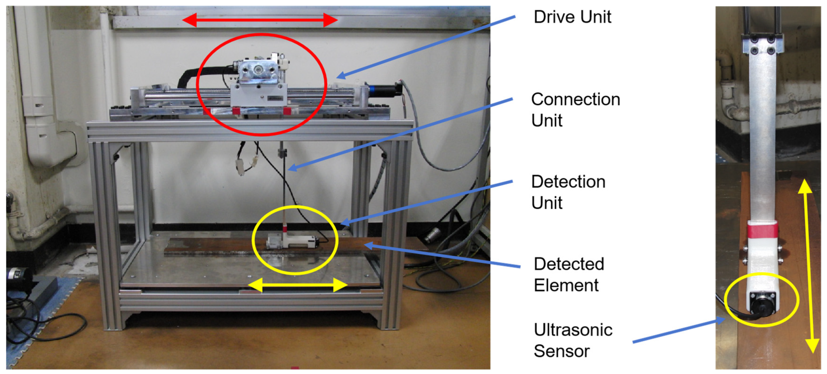
In Figure 1, the scanning detection system is a well-designed laboratory equipment specifically crafted for efficiently and accurately detecting the properties of iron plates or other materials. It is constructed with a robust metal frame and a metal tray at the bottom, ensuring its stability and durability. At the center of the system, there is a detector marked with a red circle, equipped internally with an ultrasonic sensor, capable of precisely measuring and detecting the deterioration state and thickness of materials, providing valuable data support for users. On top, a precise screw rod structure driven by a servo motor is designed, allowing users to flexibly adjust the detection position or angle, enabling the precise scanning of different areas and angles.

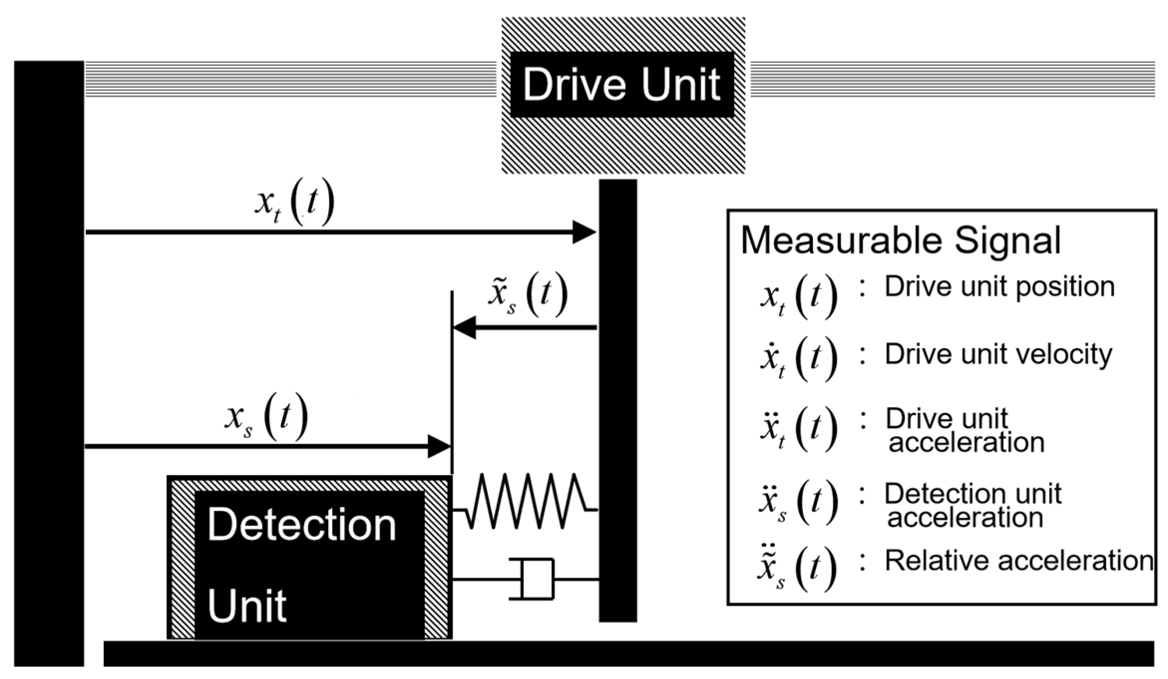
In Figure 2, a simplified model for the scanning detection system is shown. The position of the drive unit is denoted by $x_t\left(t\right)$, while its velocity and acceleration are represented by ${\dot{x}}_t\left(t\right)$ and ${\ddot{x}}_t\left(t\right)$. The input signal for the driving motor, which also serves as the control input, is designated as $u\left(t\right)$. The dynamic equation for the drive unit is presented in Equation (1). Given the insignificant impact of the detection unit on the drive unit, and considering the need to simplify the control complexity, we have omitted the direct inclusion of the detection unit’s effect in Equation (1).

$${\ddot{x}}_t(t)=-{\displaystyle \frac{c_t}{m_t}}{\dot{x}}_t(t)+{\displaystyle \frac{b_t}{m_t}}u(t)$$

(1)

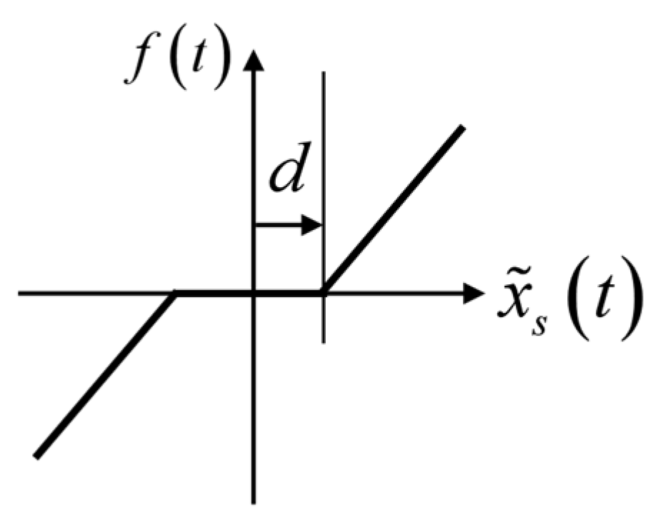
Although the drive unit and detection unit are connected by a steel strip with a certain degree of elasticity, during the modeling process, we assume that the connection between the drive unit and detection unit consists of a spring and a damper, with the spring having an elastic coefficient of $k_s$ and the damper having a damping coefficient of $c_s$. Due to the impact of contact friction between the detection unit and the object being detected, we introduce a nonlinear quantity $f\left(t\right)$, which accounts for the characteristics of both the spring and the damper, incorporates a dead zone $d$, and demonstrates the friction occurring within the sensor component, as illustrated in Figure 3. Therefore, the dynamic characteristics of the detection unit are represented in the following Equation (2), where ${\tilde{x}}_s\left(t\right)=x_s\left(t\right)-x_t\left(t\right)$ represents the relative position between the drive unit and detection unit.

$${\ddot{\tilde{x}}}_s(t)=f(t)-{\ddot{x}}_t(t)$$

(2)

.

$$f(t)=\{\begin{array}{ll}-{\displaystyle \frac{c_s}{m_s}}{\dot{\tilde{x}}}_s(t)-{\displaystyle \frac{k_s}{m_s}}{\tilde{x}}_s(t)-d& if \left|-{\displaystyle \frac{c_s}{m_s}}{\dot{\tilde{x}}}_s(t)-{\displaystyle \frac{k_s}{m_s}}{\tilde{x}}_s(t)\right|>d\\ 0& if 0\le \left|-{\displaystyle \frac{c_s}{m_s}}{\dot{\tilde{x}}}_s(t)-{\displaystyle \frac{k_s}{m_s}}{\tilde{x}}_s(t)\right|\le d\\ -{\displaystyle \frac{c_s}{m_s}}{\dot{\tilde{x}}}_s(t)-{\displaystyle \frac{k_s}{m_s}}{\tilde{x}}_s(t)+d& if \left|-{\displaystyle \frac{c_s}{m_s}}{\dot{\tilde{x}}}_s(t)-{\displaystyle \frac{k_s}{m_s}}{\tilde{x}}_s(t)\right|<-d\end{array}$$

(3)

Additionally, the explanation of symbols used in the following equations is presented in

Table 1. Symbol representation of scanning detection system.

$x_t$	Drive unit position
${\tilde{x}}_s$	The position of detection unit relative to drive unit
$m_t,m_s$	The mass of drive unit and detection unit
$b_t,c_t$	Motor input gain and viscosity resistance
$k_s,c_s$	Spring constant and damping constant
$u$	Control input

, and the nominal values of the parameters are shown in

Table 2. Simulation parameters.

Parameter	Value	Parameter	Value	Parameter	Value
${\displaystyle \frac{b_t}{m_t}}$	0.55	${\displaystyle \frac{k_s}{m_s}}$	2518	$d$	0.9
${\displaystyle \frac{c_t}{m_t}}$	0.55	${\displaystyle \frac{c_s}{m_s}}$	1.88

.

The aim of this study is to reduce the vibrations of the detection unit, which can also be translated into minimizing the oscillations in the relative position between the drive unit and the detection unit, specifically by decreasing the amplitude of the signal ${\tilde{x}}_s\left(t\right)$. This will enable the detection unit to move and perform deductions more smoothly. In order to achieve this goal, we make the following assumptions about the controlled object:

• A1. By reading the data from the servo system of the drive unit, we can obtain information on the position and velocity of the drive unit. Therefore, we assume that the position $x_t\left(t\right)$ and velocity ${\dot{x}}_t\left(t\right)$ of the drive unit are measurable;
• A2. The detection unit does not have a position sensor installed, and therefore, the position $x_s\left(t\right)$ and velocity ${\dot{x}}_s\left(t\right)$ of the detection unit cannot be measured;
• A3. Both the drive unit and detection unit are equipped with acceleration sensors, and therefore, the acceleration signals ${\ddot{x}}_t\left(t\right)$ and ${\ddot{x}}_s\left(t\right)$ are both measurable. Moreover, the relative acceleration ${\ddot{\tilde{x}}}_s\left(t\right)$ is also an available signal.

3. Oscillation Suppression Control Scheme

Although the dynamic model for the detection system was introduced in the previous section, due to the presence of nonlinear components and in order to simplify the development of the oscillation suppression controller, we will consider the following linearized model:

$${\ddot{x}}_t(t)=-{\displaystyle \frac{c_t}{m_t}}{\dot{x}}_t(t)+{\displaystyle \frac{b_t}{m_t}}u(t)$$

(4)

$${\ddot{\tilde{x}}}_s(t)=-{\displaystyle \frac{c_s}{m_s}}{\dot{\tilde{x}}}_s(t)-{\displaystyle \frac{k_s}{m_s}}{\tilde{x}}_s(t)-{\ddot{x}}_t(t)$$

(5)

where $c_s$ is a small damping constant and $k_s$ is a spring constant. The motor input signal $u\left(t\right)$ is utilized as the control input.

In Equation (5), if the signal ${\ddot{x}}_t\left(t\right)$ can be used as a virtual control input, we can make ${\ddot{x}}_t\left(t\right)$ to track the following signal,

$${\ddot{x}}_t(t)=\alpha {\dot{\tilde{x}}}_s(t)$$

(6)

where $\alpha$ is a positive design parameter. Then, we can obtain the following relation

$${\ddot{\tilde{x}}}_s(t)=-{\displaystyle \frac{c_s}{m_s}}{\dot{\tilde{x}}}_s(t)-{\displaystyle \frac{k_s}{m_s}}{\tilde{x}}_s(t)-\alpha {\dot{\tilde{x}}}_s(t)+{\Delta }_{xt},\hspace{1em}\hspace{1em}{\Delta }_{xt}=-{\ddot{x}}_t(t)+\alpha {\dot{\tilde{x}}}_s(t)$$

(7)

where ${\Delta }_{xs}$ represents the difference between ${\ddot{x}}_t(t)$ and $\alpha {\dot{\tilde{x}}}_s(t)$. After organizing and calculating the above equation, we can obtain the following relationship satisfied by the signal ${\tilde{x}}_s\left(t\right)$.

$${\tilde{X}}_s\left(s\right)={\displaystyle \frac{1}{\left(s^2+\left(\frac{c_s}{m_s}+\alpha \right)s+\frac{k_s}{m_s}\right)}}\mathsf{\Gamma }\left[{\Delta }_{xt}\right]$$

(8)

where ${\tilde{X}}_s\left(s\right)$ denotes the Laplace transform of the signal ${\tilde{x}}_s\left(t\right)$, and $\mathsf{\Gamma }[•]$ denotes the Laplace transform of the signal $•$. From Equation (8), it can be seen that the parameter $\alpha$ can adjust the convergence rate of the signal ${\tilde{x}}_s\left(t\right)$. Furthermore, if ${\Delta }_{xt}$ can converge to zero, then the signal ${\tilde{x}}_s\left(t\right)$ can also converge to zero. However, according to Assumption A2, the relative velocity ${\dot{\tilde{x}}}_s\left(t\right)$ is unavailable, and the relation shown in Equation (6) can not be directly utilized. Furthermore, in reality, ${\ddot{x}}_t\left(t\right)$ is not used as an input signal in this control system.

To overcome these above issues, the following new error signal is defined:

$${\ddot{\tilde{x}}}_t(t)={\ddot{x}}_t(t)-\alpha {\mathsf{\Gamma }}^{-1}\left[{\displaystyle \frac{Ts}{Ts+1}}{\displaystyle \frac{Ts}{Ts+1}}\mathsf{\Gamma }\left[{\dot{\tilde{x}}}_s(t)\right]\right]-{\dot{v}}_{td}(t)$$

(9)

where $T$ is a design parameter, and ${\mathsf{\Gamma }}^{-1}[•]$ denotes the inverse Laplace transform of the signal $•$. It can be seen that the second term on the right-hand side of Equation (9) represents the well-designed filtered signal of the signal $\alpha {\dot{\tilde{x}}}_s(t)$. Additionally, in order to enable the velocity signal ${\dot{x}}_t(t)$ of the drive unit to track the reference velocity signal $v_{td}(t)$, we have added the third term on the right-hand side of Equation (9). Here, $v_{td}(t)$ is the designed reference velocity signal. Moreover, the ideal velocity $v_{td}\left(t\right)$ for the drive unit is given by the following equation:

$$V_{td}\left(s\right)={\displaystyle \frac{{\omega }^2}{s^2+2\xi \omega s+{\omega }^2}}{V}_d\left(s\right)$$

(10)

where $\omega$ and $\xi$ are design parameters, and $V_d\left(s\right)=L\left[v_d\left(t\right)\right]$ is the final constant speed. It should be noted that the second term on the right-hand side of Equation (9) requires a velocity signal ${\dot{\tilde{x}}}_s(t)$. However, in our study, this velocity signal ${\dot{\tilde{x}}}_s(t)$ is not available. Therefore, we use the following equation to generate this velocity signal from the acceleration signal ${\ddot{\tilde{x}}}_s(t)$ instead:

$${\displaystyle \frac{Ts}{Ts+1}}{\displaystyle \frac{Ts}{Ts+1}}\mathsf{\Gamma }\left[{\dot{\tilde{x}}}_s(t)\right]={\displaystyle \frac{Ts}{Ts+1}}{\displaystyle \frac{T}{Ts+1}}\mathsf{\Gamma }\left[{\ddot{\tilde{x}}}_s(t)\right]$$

(11)

By substituting the content of (9) with the new signal (11), we can obtain the following equation:

$${\ddot{\tilde{x}}}_t(t)={\ddot{x}}_t(t)-\alpha {\mathsf{\Gamma }}^{-1}\left[{\displaystyle \frac{Ts}{Ts+1}}{\displaystyle \frac{T}{Ts+1}}\mathsf{\Gamma }\left[{\ddot{\tilde{x}}}_s(t)\right]\right]-{\dot{v}}_{td}(t)$$

(12)

After introducing the new signal ${\tilde{x}}_t(t)$ mentioned above, we need to analyze the impacts of ${\tilde{x}}_t(t)$ and $v_{td}(t)$ on the convergence performance of ${\tilde{x}}_s\left(t\right)$. By combining Equations (5) and (12), we obtain the following transfer function:

$$\mathsf{\Gamma }\left[{\tilde{x}}_s(t)\right]=G_s(s)\left(\mathsf{\Gamma }\left[{\ddot{\tilde{x}}}_t(t)+{\dot{v}}_{td}(t)\right]\hspace{0.17em}\right)$$

(13)

$$\begin{array}{l}{G}_s(s)=-{\displaystyle \frac{{\left(Ts+1\right)}^2}{T^2\left(s^4+A_4{s}^3+A_3{s}^2+A_{2}s+A_1\right)}}\\ A_4={\displaystyle \frac{c_s}{m_s}}+\alpha +{\displaystyle \frac{2}{T}},\hspace{1em}{A}_3={\displaystyle \frac{k_s}{m_s}}+2{\displaystyle \frac{c_s}{m_s}}{\displaystyle \frac{1}{T}}+{\displaystyle \frac{1}{T^2}}\\ A_2=2{\displaystyle \frac{k_s}{m_s}}{\displaystyle \frac{1}{T}}+{\displaystyle \frac{c_s}{m_s}}{\displaystyle \frac{1}{T^2}},\hspace{1em}{A}_1={\displaystyle \frac{k_s}{m_s}}{\displaystyle \frac{1}{T^2}}\end{array}\}$$

(14)

The derivation of Equation (13) is shown in Appendix A. It is easy to confirm that $A_i,i=1,2,3,4$ are all positive constants. Therefore, it easy to adjust the values of the design parameter $\alpha$ to make the transfer function $G_s\left(s\right)$ asymptotically stable, as demonstrated in the derivation for Equation (13). Since the ideal acceleration ${\dot{v}}_{td}\left(t\right)$ of the drive unit is designed to converge to zero, if ${\ddot{\tilde{x}}}_t(t)$ can converge to zero as well, then ${\tilde{x}}_s(t)$ will also become asymptotically stable. To achieve this and analyze the convergence performance of signal ${\ddot{\tilde{x}}}_t(t)$, a new state $x\left(t\right)={\left[\begin{array}{cc}{\dot{\tilde{x}}}_t\left(t\right)& {\ddot{\tilde{x}}}_t\left(t\right)\end{array}\right]}^T$ needs to be introduced. Using this new state variable, we obtain

$$\dot{x}=Ax+B\left(\dot{u}+\beta u\right)+Cz+D{V}_{td}$$

(15)

$$\dot{z}=A_{z}z+B_{z}x(t)+{\mathrm{C}}_z{v}_d(t)$$

(16)

$$\begin{array}{l}A=\left[\begin{array}{cc}0& 1\\ -{\displaystyle \frac{c_t}{m_t}}\beta & \left(-\beta -{\displaystyle \frac{c_t}{m_t}}+\alpha \right)\end{array}\right],B=\left[\begin{array}{c}0\\ {\displaystyle \frac{b_t}{m_t}}\end{array}\right],D=\left[\begin{array}{ccc}0& 0& 0\\ -{\displaystyle \frac{c_t}{m_t}}\beta & -\beta -{\displaystyle \frac{c_t}{m_t}}+\alpha & -1\end{array}\right],V_{td}=\left[\begin{array}{c}{v}_{td}(t)\\ {\dot{v}}_{td}(t)\\ {\ddot{v}}_{td}(t)\end{array}\right],\\ C=\left[\begin{array}{cccc}0& 0& 0& 0\\ \left({\displaystyle \frac{k_s}{m_s{T}^2}}\right)\alpha & \left({\displaystyle \frac{c_s}{m_s{T}^2}}+{\displaystyle \frac{2k_s}{m_{s}T}}\right)\alpha & \left({\displaystyle \frac{2c_s}{T{m}_s}}+{\displaystyle \frac{k_s}{m_s}}+\alpha +{\displaystyle \frac{1}{T^2}}-{\displaystyle \frac{c_t}{m_t}}\beta \right)\alpha & \left(-\beta -{\displaystyle \frac{c_t}{m_s}}+{\displaystyle \frac{c_s}{m_s}}+{\displaystyle \frac{2}{T}}\right)\alpha \end{array}\right]\\ z={\left[\begin{array}{cccc}{\left({\displaystyle \frac{Ts}{Ts+1}}\right)}^2{\displaystyle \frac{{\tilde{X}}_s}{s^2}}& {\left({\displaystyle \frac{Ts}{Ts+1}}\right)}^2{\displaystyle \frac{{\tilde{X}}_s}{s}}& {\left({\displaystyle \frac{Ts}{Ts+1}}\right)}^2{\tilde{X}}_s& {\left({\displaystyle \frac{Ts}{Ts+1}}\right)}^{2}s{\tilde{X}}_s\end{array}\right]}^T\end{array}\}$$

$$A_z=\left[\begin{array}{cccc}0& 1& 0& 0\\ 0& 0& 1& 0\\ 0& 0& 0& 1\\ -{\displaystyle \frac{k_s}{m_s{T}^2}}& -{\displaystyle \frac{c_s}{m_s{T}^2}}-{\displaystyle \frac{2k_s}{m_{s}T}}& -{\displaystyle \frac{2c_s}{T{m}_s}}-{\displaystyle \frac{k_s}{m_s}}-\alpha -{\displaystyle \frac{1}{T^2}}& -{\displaystyle \frac{c_s}{m_s}}-{\displaystyle \frac{2}{T}}\end{array}\right],B_z=\left[\begin{array}{cc}0& 0\\ 0& 0\\ 0& 0\\ 0& -1\end{array}\right],{\mathrm{C}}_z=\left[\begin{array}{ccc}0& 0& 0\\ 0& 0& 0\\ 0& 0& 0\\ 0& -1& 0\end{array}\right]\}$$

where $A_z$ is an asymptotically stable matrix. The derivation of Equation (15) is shown in Appendix B. Based on this system, we have developed the following controller:

$$\dot{u}=-\beta u-\left[\begin{array}{cc}{\beta }^2{\displaystyle \frac{m_t}{b_t}}& 2\beta {\displaystyle \frac{m_t}{b_t}}\end{array}\right]x$$

(17)

where $\beta$ is a design parameter. By substituting Equation (17) into Equation (15), the following equation can be obtained:

$$\dot{x}=\left[\begin{array}{cc}0& 1\\ -{\displaystyle \frac{c_t}{m_t}}\beta & \left(-{\displaystyle \frac{c_t}{m_t}}+\alpha \right)\end{array}\right]x-\left[\begin{array}{cc}0& 0\\ {\beta }^2& 3\beta \end{array}\right]x+Cz+D{V}_{td}$$

(18)

After dividing both sides of the Equation (18) by $\beta$ and using the following new state

$$x_{\beta }=\left[\begin{array}{cc}1& 0\\ 0& {\beta }^{-1}\end{array}\right]x=\left[\begin{array}{c}{x}_1\\ {\beta }^{-1}{x}_2\end{array}\right]$$

(19)

we can obtain

$${\dot{x}}_{\beta }=A_{\beta }{x}_{\beta }+\beta B_{\beta }{x}_{\beta }+{\beta }^{-1}Cz+{\beta }^{-1}D{V}_{td}$$

(20)

$$\dot{z}=A_{z}z+\beta B_z{x}_{\beta }+{\mathrm{C}}_z{v}_d$$

(21)

$$A_{\beta }=\left[\begin{array}{cc}0& 0\\ -{\displaystyle \frac{c_t}{m_t}}& \left(-{\displaystyle \frac{c_t}{m_t}}+\alpha \right)\end{array}\right],B_{\beta }=\left[\begin{array}{cc}0& 1\\ -1& -3\end{array}\right]$$

The stability analysis of the control system (20) and (21) by using controller (17) is shown in the following theorem.

Theorem 1.

In the control systems (20) and (21), the design parameter $\beta$ is set to satisfy the following inequalities.

$$\begin{array}{l}{\overline{\rho }}_{12}={\lambda }_{\min }\left[Q_{\beta }\right]-{\beta }^{-1}{\overline{\rho }}_{11}-2{\beta }^{-2}{\overline{\rho }}_1-{\overline{\rho }}_5>0\\ {\overline{\rho }}_{13}={\lambda }_{\min }\left[Q_{\mathrm{z}}\right]-{\overline{\rho }}_2-{\overline{\rho }}_6>0,{\overline{\rho }}_{14}={\overline{\rho }}_4+{\overline{\rho }}_8\\ {\overline{\rho }}_{11}=2\Vert P_x{A}_{\beta }\Vert ,{\overline{\rho }}_1=2\Vert P_x{P_x}^T\Vert ,{\overline{\rho }}_2=\Vert C^{T}C\Vert ,{\overline{\rho }}_4=\Vert D^{T}D\Vert \\ {\overline{\rho }}_5=\Vert {B_z}^T{B}_z\Vert ,{\overline{\rho }}_6=2\Vert P_z{P_z}^T\Vert ,{\overline{\rho }}_8=\Vert {D_z}^T{D}_z\Vert \end{array}\}$$

(22)

where  ${\lambda }_{\min }[•]$ denotes the minimum eigenvalue of matrix  $•$ , and matrices  $P_x$ and  $P_z$ are positive definite solutions to the Lyapunov equation, as shown below.

$$\begin{array}{ll}\left(P_x{B}_{\beta }+B_{\beta }^T{P}_x\right)=-Q_{\beta },& Q_{\beta }>0\\ \left(P_z{A}_z+{A_z}^{\mathrm{T}}{P}_z\right)=-Q_z,& Q_z>0\end{array}\}$$

(23)

If the initial states are $x_{\beta }\left(0\right)=0$ and $z\left(0\right)=0$, then there exist positive constants  ${\overline{\rho }}_{22},{\overline{\rho }}_{23}$ and  ${\overline{\rho }}_{24}$ that are independent of the design parameter  $\beta$, such that

$${\Vert x_{\beta }\Vert }^2\le e^{-\beta {\overline{\rho }}_{\beta }{\overline{\rho }}_{22}t}{\overline{\rho }}_{23}+{\beta }^{-2}{\overline{\rho }}_{24}$$

(24)

where  ${\overline{\rho }}_{\beta }$ is a positive constant that increases as the design parameter  $\beta$ increases.

Proof. 

In order to analyze the control system (20) and (21), we introduce a positive definite function $V_1\left(t\right)$

$$V_1\left(t\right)=x_{\beta }^T{P}_x{x}_{\beta }+{\beta }^{-1}{z}^T{P}_{z}z$$

The time derivative of $V_1\left(t\right)$ satisfies the following relationship:

$${\dot{V}}_1\left(t\right)=2x_{\beta }^T{P}_x{\dot{x}}_{\beta }+2{\beta }^{-1}{z}^T{P}_z\dot{z}$$

(25)

By substituting Equations (20) and (21) into Equation (25), we can obtain

$${\dot{V}}_1\left(t\right)=2x_{\beta }^T{P}_x\left(A_{\beta }{x}_{\beta }+\beta B_{\beta }{x}_{\beta }+{\beta }^{-1}Cz+{\beta }^{-1}D{V}_d\right)+2{\beta }^{-1}{z}^T{P}_z\left(A_{z}z+\beta B_z{x}_{\beta }+D_z{V}_d\right)$$

By substituting the well-designed relation (23), we can obtain the following equation:

$$\begin{array}{ll}{\dot{V}}_1\left(t\right)=& -\beta x_{\beta }^T{Q}_{\beta }{x}_{\beta }+2x_{\beta }^T{P}_x{A}_{\beta }{x}_{\beta }+2{\beta }^{-1}{x}_{\beta }^T{P}_{x}Cz+2{\beta }^{-1}{x}_{\beta }^T{P}_{x}D{V}_d\\ & -{\beta }^{-1}{z}^T{Q}_{z}z+2z^T{P}_z{B}_z{x}_{\beta }+2{\beta }^{-1}{z}^T{P}_z{D}_z{V}_d\end{array}$$

Then, we can obtain the following inequality,

$$\begin{array}{l}{\dot{V}}_1\left(t\right)=-\beta \left({\lambda }_{\min }\left[Q_{\beta }\right]-{\beta }^{-1}{\overline{\rho }}_{11}-{\beta }^{-2}{\overline{\rho }}_1-{\beta }^{-2}{\overline{\rho }}_3-{\overline{\rho }}_5\right){\Vert x_{\beta }\Vert }^2-{\beta }^{-1}\left({\lambda }_{\min }\left[Q_{\mathrm{z}}\right]-{\overline{\rho }}_2-{\overline{\rho }}_6-{\overline{\rho }}_7\right){\Vert z\Vert }^2\\ \hspace{1em}\hspace{1em}\hspace{1em}\hspace{1em}+{\beta }^{-1}\left({\overline{\rho }}_4+{\overline{\rho }}_8\right){\Vert V_d\Vert }^2\\ \le -\beta {\overline{\rho }}_{12}{\Vert x_{\beta }\Vert }^2-{\beta }^{-1}{\overline{\rho }}_{13}{\Vert z\Vert }^2+{\beta }^{-1}{\overline{\rho }}_{14}{\Vert V_d\Vert }^2\end{array}$$

(26)

where ${\overline{\rho }}_i,i=12,13,14$ are positive constants independent of design parameter $\beta$. In the derivation of inequality (26), the following inequality was considered:

$$\begin{array}{l}2{\beta }^{-1}{x}_{\beta }^T{P}_{x}Cz\le {\beta }^{-1}{x}_{\beta }^T{P}_x{P_x}^T{x}^{\beta }+{\beta }^{-1}{z}^T{C}^{T}Cz\le {\beta }^{-1}{\overline{\rho }}_1{\Vert x^{\beta }\Vert }^2+{\beta }^{-1}{\overline{\rho }}_2{\Vert z\Vert }^2\\ 2{\beta }^{-1}{x}_{\beta }^T{P}_{x}D{V}_d\le {\beta }^{-1}{\overline{\rho }}_1{\Vert x_{\beta }\Vert }^2+{\beta }^{-1}{\overline{\rho }}_4{\Vert V_d\Vert }^2\\ 2z^T{P}_z{B}_z{x}_{\beta }\le \beta {\overline{\rho }}_5{\Vert x_{\beta }\Vert }^2+{\beta }^{-1}{\overline{\rho }}_6{\Vert z\Vert }^2\\ 2{\beta }^{-1}{z}^T{P}_z{D}_z{V}_d\le {\beta }^{-1}{\overline{\rho }}_6{\Vert z\Vert }^2+{\beta }^{-1}{\overline{\rho }}_8{\Vert V_d\Vert }^2\end{array}\}$$

(27)

where ${\overline{\rho }}_i,i=1,\dots ,8$ are positive constants independent of design parameter $\beta$. Utilizing (26), we obtain

$${\dot{V}}_1\left(t\right)\le -{\overline{\rho }}_{15}{V}_1\left(t\right)+{\beta }^{-1}{\overline{\rho }}_{14}{\Vert V_d\Vert }^2$$

(28)

where ${\overline{\rho }}_{15}$ is a positive constant also independent of design parameter $\beta$. From (28), it can be seen that the control system becomes stable, and furthermore, $V_1\left(t\right)\le e^{-{\overline{\rho }}_{15}t}{\overline{\rho }}_{16}+{\overline{\rho }}_{17}$, ${\overline{\rho }}_{16}$ and ${\overline{\rho }}_{17}$ are positive constants that are independent of design parameter $\beta$. Additionally, it can be concluded that there exists a positive constant ${\overline{\rho }}_{18}$, also independent of design parameter $\beta$, such that $\Vert z\left(t\right)\Vert \le {\overline{\rho }}_{18}$. From the above analysis, we can confirm that the signals $x_{\beta }\left(t\right)$ and $z\left(t\right)$ are all bounded, and the control system is stable when using the proposed controller.

To further analyze the detailed control performance of the control system, we consider the positive definite function $V_2=x_{\beta }^T{P}_x{x}_{\beta }$, and by taking its derivative, we can obtain

$$\begin{array}{l}{\dot{V}}_2=2x_{\beta }^T{P}_x{\dot{x}}_{\beta }\\ =2x_{\beta }^T{P}_x{A}_{\beta }{x}_{\beta }+\beta x_{\beta }^T\left(P_x{B}_{\beta }+B_{\beta }^T{P}_x\right)x_{\beta }+2{\beta }^{-1}{x}_{\beta }^T{P}_{x}Cz+2{\beta }^{-1}{x}_{\beta }^T{P}_{x}D{V}_d\\ =-\beta x_{\beta }^T{Q}_{\beta }{x}_{\beta }+2x_{\beta }^T{P}_x{A}_{\beta }{x}_{\beta }+2{\beta }^{-1}{x}_{\beta }^T{P}_{x}Cz+2{\beta }^{-1}{x}_{\beta }^T{P}_{x}D{V}_d\end{array}$$

Utilizing the relationship

$$\begin{array}{l}2{\beta }^{-1}{x}_{\beta }^T{P}_{x}Cz\le {\beta }^{-1}{x}_{\beta }^T{P}_x{P_x}^T{x}^{\beta }+{\beta }^{-1}{z}^T{C}^{T}Cz\le {\beta }^{-1}{\overline{\rho }}_1{\Vert x_{\beta }\Vert }^2+{\beta }^{-1}{\overline{\rho }}_2{\Vert z\Vert }^2\\ 2{\beta }^{-1}{x}_{\beta }^T{P}_{x}D{V}_d\le {\beta }^{-1}{\overline{\rho }}_1{\Vert x_{\beta }\Vert }^2+{\beta }^{-1}{\overline{\rho }}_4{\Vert V_d\Vert }^2\end{array}\}$$

we can obtain

$$\begin{array}{l}{\dot{V}}_2\le -\beta {\lambda }_{\min }\left[Q_{\beta }\right]{\Vert x_{\beta }\Vert }^2+{\overline{\rho }}_{11}{\Vert x_{\beta }\Vert }^2+2{\beta }^{-1}{\overline{\rho }}_1{\Vert x_{\beta }\Vert }^2+{\beta }^{-1}{\overline{\rho }}_2{\Vert z\Vert }^2+{\beta }^{-1}{\overline{\rho }}_4{\Vert V_d\Vert }^2\\ \le -{\displaystyle \frac{\beta {\overline{\rho }}_{\beta }}{{\lambda }_{\max }\left[P_x\right]}}{x}_{\beta }^T{P}_x{x}_{\beta }+{\beta }^{-1}{\overline{\rho }}_{19}\left({\Vert z\Vert }^2+{\Vert V_d\Vert }^2\right)\le -{\displaystyle \frac{\beta {\overline{\rho }}_{\beta }}{{\lambda }_{\max }\left[P_x\right]}}{x}_{\beta }^T{P}_x{x}_{\beta }+{\beta }^{-1}{\overline{\rho }}_{20}\\ {\overline{\rho }}_{\beta }={\lambda }_{\min }\left[Q_{\beta }\right]-{\beta }^{-1}{\overline{\rho }}_{11}-2{\beta }^{-2}{\overline{\rho }}_1\end{array}$$

(29)

where ${\overline{\rho }}_{19}$ and ${\overline{\rho }}_{20}$ are positive constants unrelated to the design parameter $\beta$. According to (29), ${\overline{\rho }}_{\beta }$ is a positive value. Therefore, from (29), we can derive inequality (24). □

According to this theorem, it can be concluded that by setting the value of the design parameter $\beta$, the absolute values of ${\dot{\tilde{x}}}_t\left(t\right)$ and ${\ddot{\tilde{x}}}_t\left(t\right)$ can be reduced. Then, based on Equation (12), the state signal ${\ddot{x}}_t\left(t\right)$ will track the signal $\alpha {\ddot{\tilde{x}}}_s(t)+{\dot{v}}_{td}(t)$. Therefore, based on Equation (8), we can confirm that the detection unit’s position signal ${\tilde{x}}_s\left(t\right)$ can also be stable, and the movement speed of the drive unit is also achieved.

4. Simulation Results

Through numerical simulations, the effectiveness of the developed controller is demonstrated. Systems (1) and (2) are used as the dynamic equations of the controlled objects. The values of the system parameters are shown in Table 2. The design parameters, excluding $\beta$, are set to $\omega =11,\xi =1,T=0.1$ and $\alpha =60$. The final desired speed of the driving component is set to $V_d=0.05 \left[\mathrm{m}/\mathrm{s}\right]$. 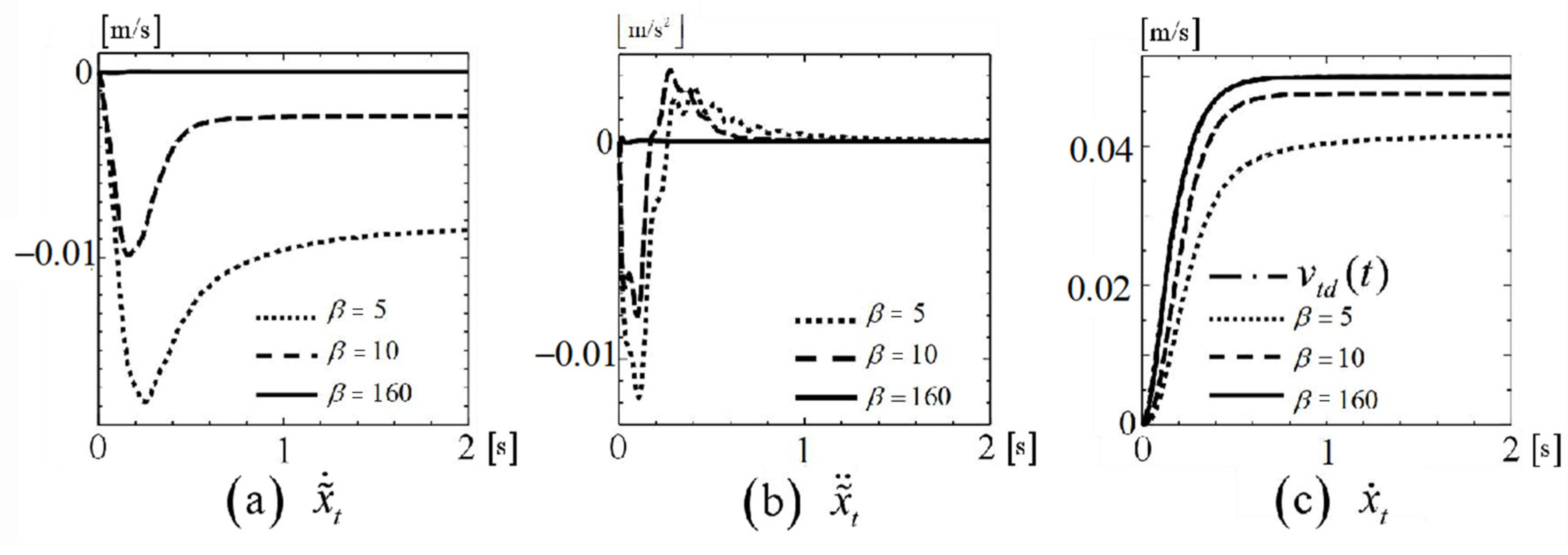Figure 4 shows the responses when the design parameter $\beta =5,10,160$. Figure 4a,b display the responses of signals ${\dot{\tilde{x}}}_t\left(t\right)$ and ${\ddot{\tilde{x}}}_t\left(t\right)$, respectively. Figure 4c shows the response of the desired speed $v_{td}$ of the driving component and the actual speed ${\dot{x}}_t\left(t\right)$ of the drive unit.

As shown in Figure 4a,b, by increasing the value of $\beta$, the maximum absolute values of ${\dot{\tilde{x}}}_t\left(t\right)$ and ${\ddot{\tilde{x}}}_t\left(t\right)$ become smaller. As depicted in Figure 4a,c, when $\beta$ is set to 160, the absolute value of ${\dot{\tilde{x}}}_t\left(t\right)$ is almost zero, with ${\dot{x}}_t\left(t\right)$ following $v_{td}$.

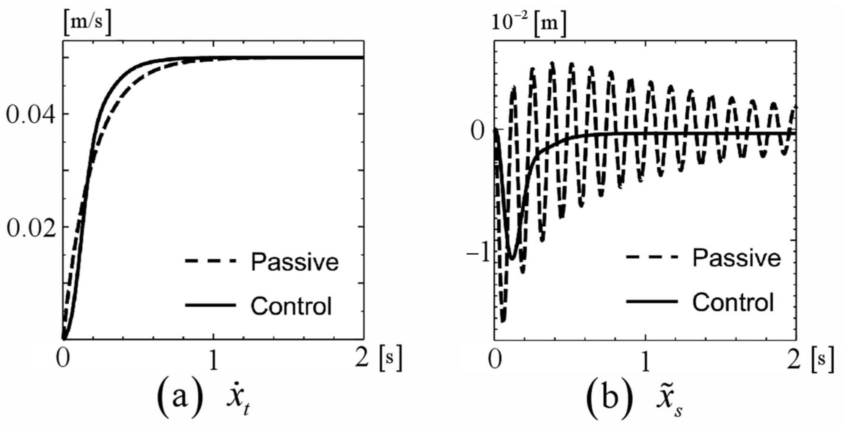
Figure 5 compares the response of the system when control is applied with $\beta =160$ (hereinafter referred to as the controlled system) with the response when no control is applied with a constant input ($u=29.2$) (hereinafter referred to as the passive system). As shown in Figure 5, compared to the passive system, the speed of the driving component in the controlled system converges rapidly to the desired value $0.05 \left[\mathrm{m}/\mathrm{s}\right]$. Furthermore, as illustrated in Figure 5b, oscillations are observed in the passive system, but these oscillations can be controlled in the controlled system.

5. Vibration Suppression Control Experiment

Based on the vibration suppression control algorithm proposed in this paper, a scanning test was conducted on an iron plate with an uneven surface, verifying the effectiveness of the proposed vibration suppression method.

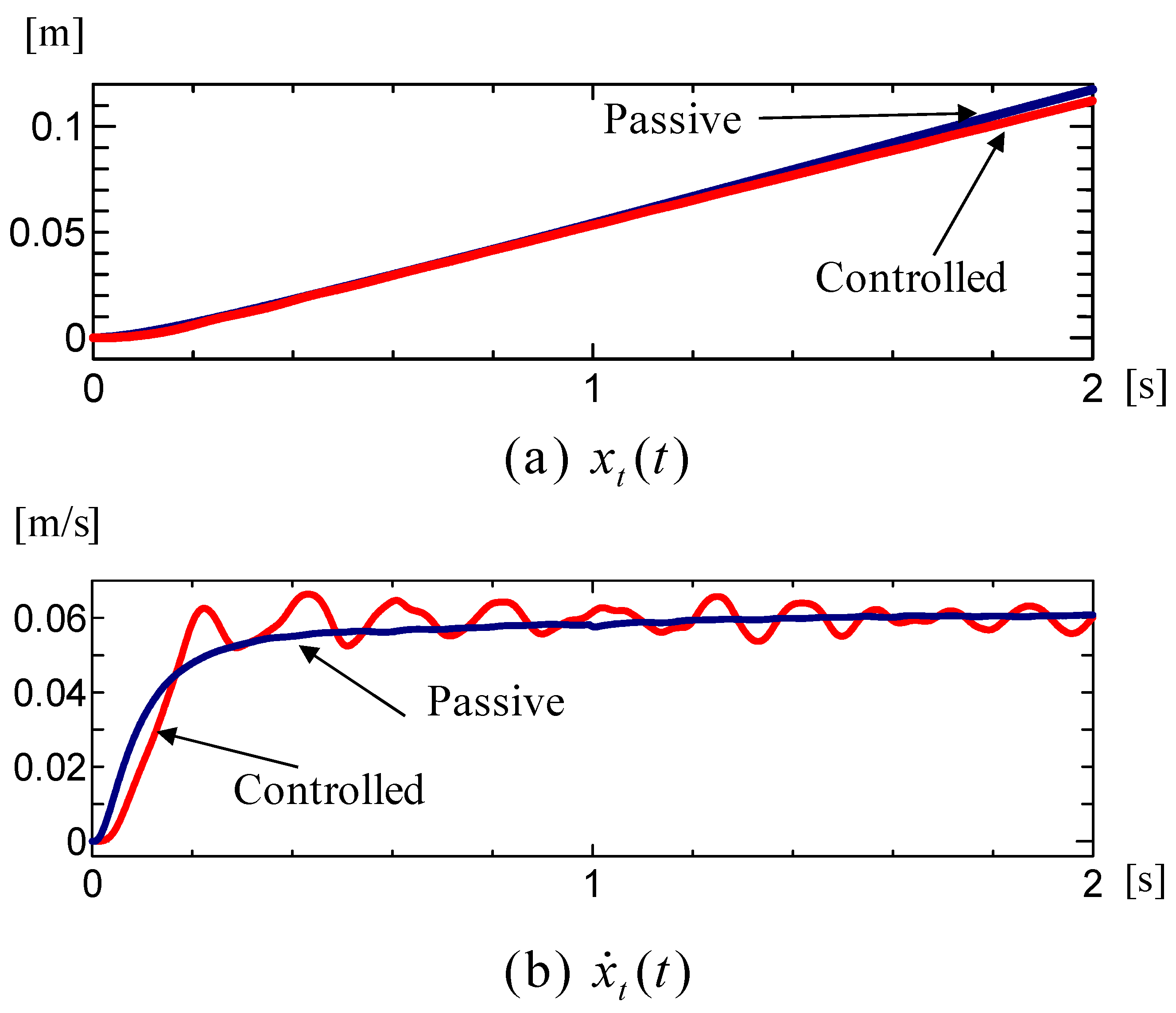
The responses of the controlled system and the passive system are shown in Figure 6 and Figure 7, respectively. Additionally, in the passive system, the input was adjusted to achieve a final velocity of 0.06 m/s for the driving unit. Figure 6a represents the position response of the driving unit, while Figure 6b depicts the velocity response of the driving unit.

As can be seen from Figure 6a,b, the control system represented by the red line is able to regulate the speed of the drive unit to a vicinity of the target value of 0.06 m/s. At this point, the position $x_t\left(t\right)$ of the drive unit exhibits a response that is roughly the same as that of the passive system represented by the blue line. Furthermore, Figure 7a compares the detected relative acceleration signal ${\ddot{\tilde{x}}}_s\left(t\right)$ with those measured in the passive system, revealing that vibrations have been effectively suppressed. Figure 7b displays the corresponding input signals $u\left(t\right)$ to the drive unit in both the controlled system and the passive system.

6. Conclusions

In this study, we have successfully proposed a vibration suppression control technique for a contact scanning sensor system utilizing accelerometers, grounded in linearized dynamic equations. Our numerical simulations of the nonlinear controlled object demonstrate the effectiveness of the developed controller, revealing that it can significantly prevent vibration in the detection part during high-speed scanning. These findings not only consolidate the theoretical underpinnings of our approach, but also highlight its practical implications for enhancing the performance of contact scanning sensor systems.

Moreover, our control method is versatile and promising for related applications. Its principles can guide future research on friction-induced vibrations. Researchers can apply this technique to precision machining and optical scanning. Based on our study, future work can explore new control methodologies for more effective vibration mitigation. Our conclusion validates the technique and sets a platform for further advancements.