
MOLA: Enhancing Industrial Process Monitoring Using a Multi-Block Orthogonal Long Short-Term Memory Autoencoder


Abstract
1. Introduction
- We introduce a novel autoencoder architecture, OLAE, to extract non-redundant and mutually independent dynamic features. Compared to existing autoencoder designs, OLAE demonstrates superior fault detection performance.
- We incorporate a state-of-the-art quantile-based multivariate CUSUM to our combined statistics to enable fast, accurate, and robust detection of process anomalies based on the mean shift in the distribution of extracted features.
- We propose a novel W-BF approach to dynamically adjust the weights assigned to monitoring results from different blocks, which significantly enhances fault detection speed and accuracy.
2. Theory and Methods
2.1. LSTM
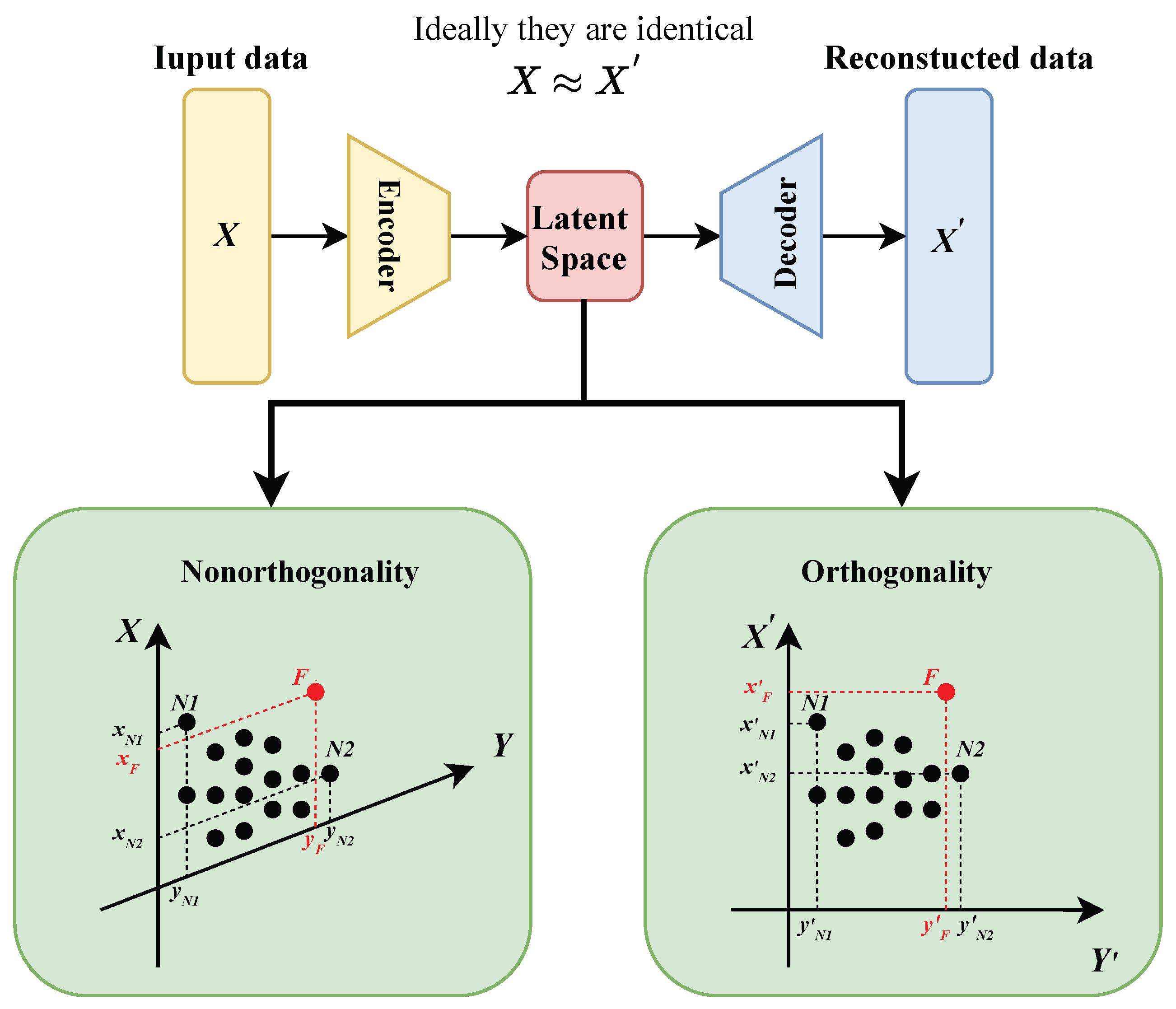
2.2. OLAE
2.3. Monitoring Statistics
2.4. Adaptive Weight-Based Bayesian Fusion Strategy
3. The MOLA Fault Detection Framework
- Step 1:
- Historical in-control data are collected, normalized, and standardized.
- Step 2:
- Based on process knowledge, process variables are divided into blocks. For each block, we establish a local OLAE model. We use 70% of the historical in-control data to build the OLAE model, whereas the remaining data serve as the validation set to determine the optimal hyperparameters for the model.
- Step 3:
- The validation data are sent to the OLAE model of each block to obtain the corresponding latent features or codes. Then, we calculate and W for each block and determine their control limits.
- Step 4:
- For each block, we implement the adaptive W-BF strategy to obtain a fused monitoring statistic.
- Step 5:
- Based on the fused monitoring statistics of each block, we apply the adaptive W-BF technique again to determine the PFI for the overall process.
- Step 1:
- As online data are collected, they are standardized based on the mean and variance of the in-control data collected during the offline learning phase.
- Step 2:
- Following the block assignments, standardized online data are sent to their corresponding block’s OLAE model to obtain the codes and monitoring statistics and W.
- Step 3:
- The fused monitoring statistic is calculated following the adaptive W-BF strategy for each block.
- Step 4:
- Using the adaptive W-BF method again, we obtain the process-level PFI from the local statistics of all blocks. If the PFI is greater than our pre-defined significance level (0.01), a fault is declared; otherwise, the process is under normal operation, and the monitoring continues.
4. Case Study
Ablation Studies Evaluating the Contribution of MOLA Components to Its Process Monitoring Performance
5. Conclusions
Author Contributions
Funding
Institutional Review Board Statement
Informed Consent Statement
Data Availability Statement
Conflicts of Interest
References
- Amin, M.T.; Imtiaz, S.; Khan, F. Process system fault detection and diagnosis using a hybrid technique. Chem. Eng. Sci. 2018, 189, 191–211. [Google Scholar] [CrossRef]
- Nawaz, M.; Maulud, A.S.; Zabiri, H.; Suleman, H. Review of multiscale methods for process monitoring, with an emphasis on applications in chemical process systems. IEEE Access 2022, 10, 49708–49724. [Google Scholar] [CrossRef]
- Qin, S.J. Survey on data-driven industrial process monitoring and diagnosis. Annu. Rev. Control. 2012, 36, 220–234. [Google Scholar] [CrossRef]
- Li, S.; Luo, J.; Hu, Y. Nonlinear process modeling via unidimensional convolutional neural networks with self-attention on global and local inter-variable structures and its application to process monitoring. ISA Trans. 2022, 121, 105–118. [Google Scholar] [CrossRef]
- Dong, Y.; Qin, S.J. A novel dynamic PCA algorithm for dynamic data modeling and process monitoring. J. Process. Control 2018, 67, 1–11. [Google Scholar] [CrossRef]
- Bounoua, W.; Bakdi, A. Fault detection and diagnosis of nonlinear dynamical processes through correlation dimension and fractal analysis based dynamic kernel PCA. Chem. Eng. Sci. 2021, 229, 116099. [Google Scholar] [CrossRef]
- Pilario, K.E.; Shafiee, M.; Cao, Y.; Lao, L.; Yang, S.H. A review of kernel methods for feature extraction in nonlinear process monitoring. Processes 2019, 8, 24. [Google Scholar] [CrossRef]
- Tan, R.; Ottewill, J.R.; Thornhill, N.F. Monitoring statistics and tuning of kernel principal component analysis with radial basis function kernels. IEEE Access 2020, 8, 198328–198342. [Google Scholar] [CrossRef]
- Abiodun, O.I.; Jantan, A.; Omolara, A.E.; Dada, K.V.; Mohamed, N.A.; Arshad, H. State-of-the-art in artificial neural network applications: A survey. Heliyon 2018, 4, e00938. [Google Scholar] [CrossRef]
- Wu, H.; Zhao, J. Deep convolutional neural network model based chemical process fault diagnosis. Comput. Chem. Eng. 2018, 115, 185–197. [Google Scholar] [CrossRef]
- Arunthavanathan, R.; Khan, F.; Ahmed, S.; Imtiaz, S. A deep learning model for process fault prognosis. Process. Saf. Environ. Prot. 2021, 154, 467–479. [Google Scholar] [CrossRef]
- Heo, S.; Lee, J.H. Fault detection and classification using artificial neural networks. IFAC-PapersOnLine 2018, 51, 470–475. [Google Scholar] [CrossRef]
- Yang, Z.; Xu, B.; Luo, W.; Chen, F. Autoencoder-based representation learning and its application in intelligent fault diagnosis: A review. Measurement 2022, 189, 110460. [Google Scholar] [CrossRef]
- Ji, C.; Sun, W. A review on data-driven process monitoring methods: Characterization and mining of industrial data. Processes 2022, 10, 335. [Google Scholar] [CrossRef]
- Fan, J.; Wang, W.; Zhang, H. AutoEncoder based high-dimensional data fault detection system. In Proceedings of the 2017 IEEE 15th International Conference on Industrial Informatics (INDIN), Emden, Germany, 24–26 July 2017; pp. 1001–1006. [Google Scholar]
- Qian, J.; Song, Z.; Yao, Y.; Zhu, Z.; Zhang, X. A review on autoencoder based representation learning for fault detection and diagnosis in industrial processes. Chemom. Intell. Lab. Syst. 2022, 231, 104711. [Google Scholar] [CrossRef]
- Wang, W.; Yang, D.; Chen, F.; Pang, Y.; Huang, S.; Ge, Y. Clustering with orthogonal autoencoder. IEEE Access 2019, 7, 62421–62432. [Google Scholar] [CrossRef]
- Cacciarelli, D.; Kulahci, M. A novel fault detection and diagnosis approach based on orthogonal autoencoders. Comput. Chem. Eng. 2022, 163, 107853. [Google Scholar] [CrossRef]
- Md Nor, N.; Che Hassan, C.R.; Hussain, M.A. A review of data-driven fault detection and diagnosis methods: Applications in chemical process systems. Rev. Chem. Eng. 2020, 36, 513–553. [Google Scholar] [CrossRef]
- Ji, C.; Ma, F.; Wang, J.; Sun, W. Orthogonal projection based statistical feature extraction for continuous process monitoring. Comput. Chem. Eng. 2024, 183, 108600. [Google Scholar] [CrossRef]
- Nawaz, M.; Maulud, A.S.; Zabiri, H.; Taqvi, S.A.A.; Idris, A. Improved process monitoring using the CUSUM and EWMA-based multiscale PCA fault detection framework. Chin. J. Chem. Eng. 2021, 29, 253–265. [Google Scholar] [CrossRef]
- Ge, Z. Review on data-driven modeling and monitoring for plant-wide industrial processes. Chemom. Intell. Lab. Syst. 2017, 171, 16–25. [Google Scholar] [CrossRef]
- Huang, J.; Ersoy, O.K.; Yan, X. Fault detection in dynamic plant-wide process by multi-block slow feature analysis and support vector data description. ISA Trans. 2019, 85, 119–128. [Google Scholar] [CrossRef] [PubMed]
- Zhai, C.; Sheng, X.; Xiong, W. Multi-block Fault Detection for Plant-wide Dynamic Processes Based on Fault Sensitive Slow Features and Support Vector Data Description. IEEE Access 2020, 8, 120737–120745. [Google Scholar] [CrossRef]
- Li, Y.; Peng, X.; Tian, Y. Plant-wide process monitoring strategy based on complex network and Bayesian inference-based multi-block principal component analysis. IEEE Access 2020, 8, 199213–199226. [Google Scholar] [CrossRef]
- Ye, H.; Liu, K. A generic online nonparametric monitoring and sampling strategy for high-dimensional heterogeneous processes. IEEE Trans. Autom. Sci. Eng. 2022, 19, 1503–1516. [Google Scholar] [CrossRef]
- Jiang, Z. Online Monitoring and Robust, Reliable Fault Detection of Chemical Process Systems. In Computer Aided Chemical Engineering; Elsevier: Amsterdam, The Netherlands, 2023; Volume 52, pp. 1623–1628. [Google Scholar]
- Zhang, S.; Bi, K.; Qiu, T. Bidirectional recurrent neural network-based chemical process fault diagnosis. Ind. Eng. Chem. Res. 2019, 59, 824–834. [Google Scholar] [CrossRef]
- Deng, W.; Li, Y.; Huang, K.; Wu, D.; Yang, C.; Gui, W. LSTMED: An uneven dynamic process monitoring method based on LSTM and Autoencoder neural network. Neural Netw. 2023, 158, 30–41. [Google Scholar] [CrossRef]
- Ren, J.; Ni, D. A batch-wise LSTM-encoder decoder network for batch process monitoring. Chem. Eng. Res. Des. 2020, 164, 102–112. [Google Scholar] [CrossRef]
- Ma, F.; Wang, J.; Sun, W. A Data-Driven Semi-Supervised Soft-Sensor Method: Application on an Industrial Cracking Furnace. Front. Chem. Eng. 2022, 4, 899941. [Google Scholar] [CrossRef]
- Mao, T.; Zhang, Y.; Ruan, Y.; Gao, H.; Zhou, H.; Li, D. Feature learning and process monitoring of injection molding using convolution-deconvolution auto encoders. Comput. Chem. Eng. 2018, 118, 77–90. [Google Scholar] [CrossRef]
- Qiu, P.; Hawkins, D. A nonparametric multivariate cumulative sum procedure for detecting shifts in all directions. J. R. Stat. Soc. Ser. D Stat. 2003, 52, 151–164. [Google Scholar] [CrossRef]
- Mei, Y. Quickest detection in censoring sensor networks. In Proceedings of the 2011 IEEE International Symposium on Information Theory Proceedings, St. Petersburg, Russia, 31 July–5 August 2011; pp. 2148–2152. [Google Scholar]
- Rong, M.; Shi, H.; Song, B.; Tao, Y. Multi-block dynamic weighted principal component regression strategy for dynamic plant-wide process monitoring. Measurement 2021, 183, 109705. [Google Scholar] [CrossRef]
- Ge, Z.; Chen, J. Plant-wide industrial process monitoring: A distributed modeling framework. IEEE Trans. Ind. Inform. 2015, 12, 310–321. [Google Scholar] [CrossRef]
- Downs, J.J.; Vogel, E.F. A plant-wide industrial process control problem. Comput. Chem. Eng. 1993, 17, 245–255. [Google Scholar] [CrossRef]
- Jiang, Q.; Yan, X.; Huang, B. Review and perspectives of data-driven distributed monitoring for industrial plant-wide processes. Ind. Eng. Chem. Res. 2019, 58, 12899–12912. [Google Scholar] [CrossRef]
- Zhu, J.; Ge, Z.; Song, Z. Distributed parallel PCA for modeling and monitoring of large-scale plant-wide processes with big data. IEEE Trans. Ind. Inform. 2017, 13, 1877–1885. [Google Scholar] [CrossRef]
- Bathelt, A.; Ricker, N.L.; Jelali, M. Revision of the Tennessee Eastman process model. IFAC-PapersOnLine 2015, 48, 309–314. [Google Scholar] [CrossRef]
- Alakent, B. Early fault detection via combining multilinear PCA with retrospective monitoring using weighted features. Braz. J. Chem. Eng. 2024, 41, 1–23. [Google Scholar] [CrossRef]
- Kinney, J.B.; Atwal, G.S. Equitability, mutual information, and the maximal information coefficient. Proc. Natl. Acad. Sci. USA 2014, 111, 3354–3359. [Google Scholar] [CrossRef]


| Capability | PCA | KPCA | DPCA | AE | LSTM AE | Block PCA | Block LSTM AE | MOLA |
|---|---|---|---|---|---|---|---|---|
| Cross-correlation | ✓ | ✓ | ✓ | ✓ | ✓ | ✓ | ✓ | ✓ |
| Dynamic | × | × | ✓ | × | ✓ | × | ✓ | ✓ |
| Nonlinearity | × | ✓ | × | ✓ | ✓ | × | ✓ | ✓ |
| Orthogonality | ✓ | ✓ | ✓ | × | × | ✓ | × | ✓ |
| Large-scale monitoring | × | × | × | × | × | ✓ | ✓ | ✓ |
| Adaptive Weight | × | × | × | × | × | × | × | ✓ |
| Distribution monitoring | × | × | × | × | × | × | × | ✓ |
| No. | Variable | Description | No. | Variable | Description |
|---|---|---|---|---|---|
| 0 | FI-1001 | A feed (stream 1) | 16 | FI-1009 | Stripper underflow (stream 11) |
| 1 | FI-1002 | D feed (stream 2) | 17 | TI-1003 | Stripper temperature |
| 2 | FI-1003 | E feed (stream 3) | 18 | FI-1010 | Stripper steam flow |
| 3 | FI-1004 | A and C feed (stream 4) | 19 | JI-1001 | Compressor work |
| 4 | FI-1005 | Recycle flow (stream 8) | 20 | TI-1004 | Reactor cooling water outlet temperature |
| 5 | FI-1006 | Reactor feed rate (stream 6) | 21 | TI-1005 | Separator cooling water outlet temperature |
| 6 | PI-1001 | Reactor pressure | 22 | FIC-1001 | D feed flow (stream 2) |
| 7 | LI-1001 | Reactor level | 23 | FIC-1002 | E feed flow (stream 3) |
| 8 | TI-1001 | Reactor temperature | 24 | FIC-1003 | A feed flow (stream 1) |
| 9 | FI-1007 | Purge rate (stream 9) | 25 | FIC-1004 | A and C feed flow (stream 4) |
| 10 | TI-1002 | Product separator temperature | 26 | FV-1001 | Purge valve (stream 9) |
| 11 | LI-1002 | Product separator level | 27 | FIC-1005 | Separator pot liquid flow (stream 10) |
| 12 | PI-1002 | Product separator pressure | 28 | FIC-1006 | Stripper liquid prod flow (stream 11) |
| 13 | FI-1008 | Product separator underflow (stream 10) | 29 | FIC-1007 | Reactor cooling water flow |
| 14 | LI-1003 | Stripper level | 30 | FIC-1008 | Condenser cooling water flow |
| 15 | PI-1003 | Stripper pressure |
| Block | Variables | Description |
|---|---|---|
| 1 | 0, 1, 2, 4, 5, 22, 23, 24 | Input |
| 2 | 6, 7, 8, 20, 29 | Reactor |
| 3 | 9, 10, 11, 12, 13, 19, 21, 26, 27, 30 | Separator, compressor and condenser |
| 4 | 3, 14, 15, 16, 17, 18, 25, 28 | Stripper |
| Fault No. | Process Variable | Type |
|---|---|---|
| 1 | A/C feed ratio, B composition constant (stream 4) | Step |
| 2 | B composition, A/C ratio constant (stream 4) | Step |
| 3 | D feed temperature (stream 2) | Step |
| 4 | Reactor cooling water inlet temperature | Step |
| 5 | Condenser cooling water inlet temperature | Step |
| 6 | A feed loss (stream 1) | Step |
| 7 | C header pressure loss-reduced availability (stream 4) | Step |
| 8 | A, B, C feed composition (stream 4) | Random variation |
| 9 | D feed temperature (stream 2) | Random variation |
| 10 | C feed temperature (stream 4) | Random variation |
| 11 | Reactor cooling water inlet temperature | Random variation |
| 12 | Condenser cooling water inlet temperature | Random variation |
| 13 | Reaction kinetics | Slow drift |
| 14 | Reactor cooling water valve | Sticking |
| 15 | Condenser cooling water valve | Sticking |
| 16 | Unknown | Unknown |
| 17 | Unknown | Unknown |
| 18 | Unknown | Unknown |
| 19 | Unknown | Unknown |
| 20 | Unknown | Unknown |
| Model | Structure | Activation Function |
|---|---|---|
| AE | FC(64)-FC(16)-FC(64) | ReLU |
| LSTM AE | LSTM(64)-FC(16)-LSTM(64) | ReLU |
| Block LSTM AE | LSTM(15)-FC(5)-LSTM(15) | ReLU |
| OLAE | LSTM(15)-FC(5)-LSTM(15) | ReLU |
| Fault No. | PCA () | PCA (Q) | AE | LSTM AE | Block PCA () | Block PCA (Q) | Block LSTM AE | MOLA |
|---|---|---|---|---|---|---|---|---|
| 1 | 3 | 18 | 3 | 1 | 1 | 15 | 4 | 1 |
| 2 | 25 | 140 | 22 | 20 | 19 | 726 | 18 | 16 |
| 3 | – | – | – | 27 | – | – | 572 | 30 |
| 4 | 0 | 0 | 0 | 0 | 0 | 0 | 0 | 0 |
| 5 | – | – | – | 208 | 2 | – | 3 | 2 |
| 6 | 0 | 0 | 0 | 0 | 0 | 0 | 0 | 0 |
| 7 | 0 | 0 | 0 | 0 | 0 | 0 | 0 | 0 |
| 8 | 29 | 200 | 26 | 28 | 25 | 45 | 27 | 25 |
| 9 | 229 | – | – | 40 | 26 | – | 233 | 25 |
| 10 | 91 | 90 | 77 | 77 | 74 | 188 | 74 | 70 |
| 11 | 36 | 41 | 36 | 22 | 36 | 37 | 36 | 36 |
| 12 | 66 | – | 65 | 63 | 66 | 475 | 48 | 60 |
| 13 | 94 | 317 | 86 | 86 | 89 | 307 | 91 | 9 |
| 14 | – | 7 | 3 | 0 | 2 | 3 | 2 | 2 |
| 15 | 191 | – | – | – | – | – | 191 | 6 |
| 16 | – | – | – | – | – | – | – | 21 |
| 17 | 57 | 62 | 55 | 55 | 56 | 58 | 57 | 24 |
| 18 | 267 | 280 | 242 | 241 | 259 | 259 | 268 | 147 |
| 19 | 30 | 32 | 15 | 16 | 21 | 32 | 12 | 11 |
| 20 | 141 | 178 | 129 | 128 | 138 | 164 | 123 | 124 |
| No. | PCA () | PCA (Q) | AE | LSTM AE | Block PCA () | Block PCA (Q) | Block LSTM AE | MOLA | % Improvement |
|---|---|---|---|---|---|---|---|---|---|
| 1 | 0.9967 | 0.9700 | 0.9950 | 0.9967 | 0.9983 | 0.9750 | 0.9950 | 0.9983 | 0.00 |
| 2 | 0.9617 | 0.6850 | 0.9667 | 0.9650 | 0.9683 | 0.7200 | 0.9700 | 0.9767 | 0.68 |
| 3 | 0.0067 | 0.0000 | 0.0183 | 0.0467 | 0.0267 | 0.0000 | 0.0350 | 0.9567 | 1950.00 |
| 4 | 1.0000 | 1.0000 | 1.0000 | 1.0000 | 1.0000 | 1.0000 | 1.0000 | 1.0000 | 0.00 |
| 5 | 0.0183 | 0.0000 | 0.0033 | 0.0300 | 0.0350 | 0.0000 | 0.0467 | 0.2633 | 464.28 |
| 6 | 1.0000 | 1.0000 | 1.0000 | 1.0000 | 1.0000 | 1.0000 | 1.0000 | 1.0000 | 0.00 |
| 7 | 1.0000 | 1.0000 | 1.0000 | 1.0000 | 1.0000 | 1.0000 | 1.0000 | 1.0000 | 0.00 |
| 8 | 0.8500 | 0.6683 | 0.8883 | 0.8500 | 0.8883 | 0.7000 | 0.9000 | 0.9433 | 4.81 |
| 9 | 0.0300 | 0.0000 | 0.0567 | 0.0633 | 0.0517 | 0.0000 | 0.0400 | 0.8850 | 1297.37 |
| 10 | 0.6700 | 0.5367 | 0.8100 | 0.8033 | 0.8233 | 0.0400 | 0.8350 | 0.8833 | 5.79 |
| 11 | 0.9400 | 0.8417 | 0.9433 | 0.9500 | 0.9483 | 0.8600 | 0.9433 | 0.9533 | 0.35 |
| 12 | 0.3467 | 0.0000 | 0.3083 | 0.3267 | 0.4383 | 0.0100 | 0.4550 | 0.6467 | 42.12 |
| 13 | 0.8467 | 0.4167 | 0.8483 | 0.8417 | 0.8583 | 0.4133 | 0.8583 | 0.8733 | 1.75 |
| 14 | 0.9883 | 0.6567 | 0.9950 | 0.9967 | 0.9967 | 0.7833 | 0.9767 | 0.9967 | 0.00 |
| 15 | 0.0117 | 0.0000 | 0.0150 | 0.0100 | 0.0133 | 0.0000 | 0.0317 | 0.9850 | 3010.52 |
| 16 | 0.0167 | 0.0000 | 0.0117 | 0.0083 | 0.0083 | 0.0000 | 0.0250 | 0.6450 | 2480.00 |
| 17 | 0.9017 | 0.7683 | 0.9083 | 0.9100 | 0.9067 | 0.8283 | 0.9050 | 0.9233 | 2.03 |
| 18 | 0.3500 | 0.2567 | 0.4850 | 0.4817 | 0.4200 | 0.3867 | 0.3950 | 0.7633 | 57.39 |
| 19 | 0.9317 | 0.8000 | 0.9783 | 0.9683 | 0.9683 | 0.6550 | 0.9750 | 0.9817 | 0.68 |
| 20 | 0.7650 | 0.5400 | 0.7933 | 0.7900 | 0.7750 | 0.5583 | 0.7917 | 0.7933 | 0.00 |
| PCA () | PCA (Q) | AE | LSTM AE | Block PCA () | Block PCA (Q) | Block LSTM AE | MOLA | |
|---|---|---|---|---|---|---|---|---|
| FDR | 0.0017 | 0.0000 | 0.0133 | 0.0067 | 0.0067 | 0.0000 | 0.0283 | 0.0350 |
| No. | Block 1 | Block 2 | Block 3 | Block 4 | ||||
|---|---|---|---|---|---|---|---|---|
| LSTM AE | MOLA | LSTM AE | MOLA | LSTM AE | MOLA | LSTM AE | MOLA | |
| MIC(F1,F2) | 0.2637 | 0.0337 | 0.0555 | 0.0541 | 0.1278 | 0.0706 | 0.9752 | 0.0405 |
| MIC(F1,F3) | 0.7957 | 0.1558 | 0.0708 | 0.0754 | 0.0427 | 0.0590 | 0.6531 | 0.0586 |
| MIC(F1,F4) | 0.3043 | 0.0628 | 0.1924 | 0.0908 | 0.0901 | 0.0867 | 0.7901 | 0.0547 |
| MIC(F1,F5) | 0.7275 | 0.0256 | 0.0774 | 0.1182 | 0.1287 | 0.0978 | 0.9610 | 0.0438 |
| MIC(F2,F3) | 0.7238 | 0.0723 | 0.4757 | 0.0879 | 0.0712 | 0.0938 | 0.9175 | 0.0789 |
| MIC(F2,F4) | 0.6029 | 0.1292 | 0.2940 | 0.1075 | 0.0663 | 0.0916 | 0.8663 | 0.0664 |
| MIC(F2,F5) | 0.5836 | 0.0946 | 0.5009 | 0.0918 | 0.1219 | 0.0559 | 0.9773 | 0.0550 |
| MIC(F3,F4) | 0.5106 | 0.1165 | 0.3697 | 0.0595 | 0.0352 | 0.0347 | 0.8658 | 0.0480 |
| MIC(F3,F5) | 0.9525 | 0.0948 | 0.9523 | 0.0742 | 0.0523 | 0.0387 | 0.8695 | 0.0417 |
| MIC(F4,F5) | 0.4059 | 0.0397 | 0.3442 | 0.0442 | 0.0944 | 0.1517 | 0.5427 | 0.0598 |
| No. | Block 1 | Block 2 | Block 3 | Block 4 | Block LSTM AE | MOLA w/o BF and CUSUM | ||||
|---|---|---|---|---|---|---|---|---|---|---|
| LSTM AE | OLAE | LSTM AE | OLAE | LSTM AE | OLAE | LSTM AE | OLAE | |||
| 1 | 21 | 18 | 4 | 1 | 4 | 3 | 3 | 2 | 4 | 2 |
| 2 | 117 | 118 | 21 | 17 | 22 | 16 | 18 | 9 | 18 | 16 |
| 3 | - | - | - | 139 | 573 | 573 | - | - | 572 | 160 |
| 4 | - | - | 0 | 0 | 10 | 10 | - | 44 | 0 | 0 |
| 5 | - | - | - | 1 | 3 | 2 | - | 3 | 3 | 2 |
| 6 | 0 | 0 | 1 | 0 | 3 | 3 | 2 | 2 | 0 | 0 |
| 7 | - | - | 0 | 0 | 1 | 1 | 0 | 0 | 0 | 0 |
| 8 | 56 | 36 | 182 | 28 | 32 | 32 | 27 | 24 | 27 | 27 |
| 9 | - | 23 | 233 | 61 | - | 61 | - | 62 | 233 | 61 |
| 10 | - | - | - | 380 | 170 | 170 | 74 | 70 | 74 | 70 |
| 11 | - | - | 36 | 36 | 47 | 41 | 63 | 49 | 36 | 36 |
| 12 | - | 553 | 85 | 60 | 48 | 60 | 65 | 65 | 48 | 60 |
| 13 | 249 | 245 | 97 | 74 | 89 | 84 | 106 | 9 | 91 | 84 |
| 14 | - | 202 | 2 | 2 | - | 56 | - | 26 | 2 | 2 |
| 15 | - | - | - | 82 | 192 | 191 | - | 209 | 191 | 192 |
| 16 | - | - | - | - | 54 | 18 | - | 19 | - | 25 |
| 17 | - | - | 56 | 54 | 118 | 117 | 140 | 57 | 57 | 56 |
| 18 | - | - | 345 | 345 | 263 | 260 | 346 | 346 | 268 | 260 |
| 19 | - | - | 409 | 244 | 25 | 20 | 12 | 11 | 12 | 12 |
| 20 | 164 | 162 | 212 | 177 | 129 | 129 | 123 | 124 | 123 | 127 |
| Fault No. | Full MOLA | MOLA no BF | MOLA no CUSUM | |||
|---|---|---|---|---|---|---|
| FDD | FDR | FDD | FDR | FDD | FDR | |
| 1 | 1 | 0.9983 | 1 | 0.9983 | 1 | 0.9983 |
| 2 | 16 | 0.9767 | 16 | 0.9750 | 16 | 0.9750 |
| 3 | 30 | 0.9567 | 31 | 0.9550 | 139 | 0.1117 |
| 4 | 0 | 1.0000 | 0 | 1.0000 | 0 | 1.0000 |
| 5 | 2 | 0.2633 | 2 | 0.2283 | 2 | 0.0717 |
| 6 | 0 | 1.0000 | 0 | 1.0000 | 0 | 1.0000 |
| 7 | 0 | 1.0000 | 0 | 1.0000 | 0 | 1.0000 |
| 8 | 25 | 0.9433 | 25 | 0.9350 | 26 | 0.9167 |
| 9 | 25 | 0.8850 | 25 | 0.8800 | 23 | 0.1550 |
| 10 | 70 | 0.8833 | 70 | 0.8833 | 70 | 0.8567 |
| 11 | 36 | 0.9533 | 36 | 0.9500 | 36 | 0.9500 |
| 12 | 60 | 0.6467 | 60 | 0.6217 | 60 | 0.5517 |
| 13 | 09 | 0.8733 | 84 | 0.8667 | 84 | 0.8717 |
| 14 | 2 | 0.9967 | 2 | 0.9967 | 2 | 0.9967 |
| 15 | 6 | 0.9850 | 12 | 0.9550 | 192 | 0.0667 |
| 16 | 21 | 0.6450 | 25 | 0.6233 | 25 | 0.0450 |
| 17 | 24 | 0.9233 | 24 | 0.9183 | 54 | 0.9117 |
| 18 | 147 | 0.7633 | 148 | 0.7567 | 260 | 0.4567 |
| 19 | 11 | 0.9817 | 12 | 0.9800 | 11 | 0.9817 |
| 20 | 124 | 0.7933 | 124 | 0.7917 | 124 | 0.7933 |
| Average | 30.45 | 0.8734 | 30.85 | 0.8658 | 56.25 | 0.6855 |
Disclaimer/Publisher’s Note: The statements, opinions and data contained in all publications are solely those of the individual author(s) and contributor(s) and not of MDPI and/or the editor(s). MDPI and/or the editor(s) disclaim responsibility for any injury to people or property resulting from any ideas, methods, instructions or products referred to in the content. |
© 2024 by the authors. Licensee MDPI, Basel, Switzerland. This article is an open access article distributed under the terms and conditions of the Creative Commons Attribution (CC BY) license (https://creativecommons.org/licenses/by/4.0/).
Share and Cite
Ma, F.; Ji, C.; Wang, J.; Sun, W.; Tang, X.; Jiang, Z. MOLA: Enhancing Industrial Process Monitoring Using a Multi-Block Orthogonal Long Short-Term Memory Autoencoder. Processes 2024, 12, 2824. https://doi.org/10.3390/pr12122824
Ma F, Ji C, Wang J, Sun W, Tang X, Jiang Z. MOLA: Enhancing Industrial Process Monitoring Using a Multi-Block Orthogonal Long Short-Term Memory Autoencoder. Processes. 2024; 12(12):2824. https://doi.org/10.3390/pr12122824
Chicago/Turabian StyleMa, Fangyuan, Cheng Ji, Jingde Wang, Wei Sun, Xun Tang, and Zheyu Jiang. 2024. "MOLA: Enhancing Industrial Process Monitoring Using a Multi-Block Orthogonal Long Short-Term Memory Autoencoder" Processes 12, no. 12: 2824. https://doi.org/10.3390/pr12122824
APA StyleMa, F., Ji, C., Wang, J., Sun, W., Tang, X., & Jiang, Z. (2024). MOLA: Enhancing Industrial Process Monitoring Using a Multi-Block Orthogonal Long Short-Term Memory Autoencoder. Processes, 12(12), 2824. https://doi.org/10.3390/pr12122824